What is the largest Einstein radius in the universe?

Abstract

The Einstein radius plays a central role in lens studies as it characterises the strength of gravitational lensing. In particular, the distribution of Einstein radii near the upper cutoff should probe the probability distribution of the largest mass concentrations in the universe. Adopting a triaxial halo model, we compute expected distributions of large Einstein radii. To assess the cosmic variance, we generate a number of Monte-Carlo realisations of all-sky catalogues of massive clusters. We find that the expected largest Einstein radius in the universe is sensitive to parameters characterising the cosmological model, especially $\sigma_{8}$: for a source redshift of unity, they are $42{}^{+9}_{-7}$, $35{}^{+8}_{-6}$, and $54{}^{+12}_{-7}$ arcseconds (errors denote $1\sigma$ cosmic variance), assuming best-fit cosmological parameters of the Wilkinson Microwave Anisotropy Probe five-year (WMAP5), three-year (WMAP3) and one-year (WMAP1) data, respectively. These values are broadly consistent with current observations given their incompleteness. The mass of the largest lens cluster can be as small as $\sim 10^{15}M_{\odot}$. For the same source redshift, we expect in all-sky $\sim 35$ (WMAP5), $\sim 15$ (WMAP3), and $\sim 150$ (WMAP1) clusters that have Einstein radii larger than $20^{\prime\prime}$. For a larger source redshift of 7, the largest Einstein radii grow approximately twice as large. Whilst the values of the largest Einstein radii are almost unaffected by the level of the primordial non-Gaussianity currently of interest, the measurement of the abundance of moderately large lens clusters should probe non-Gaussianity competitively with cosmic microwave background experiments, but only if other cosmological parameters are well-measured. These semi-analytic predictions are based on a rather simple representation of clusters, and hence calibrating them with $N$-body simulations will help to improve the accuracy. We also find that these “superlens” clusters constitute a highly biased population. For instance, a substantial fraction of these superlens clusters have major axes preferentially aligned with the line-of-sight. As a consequence, the projected mass distributions of the clusters are rounder by an ellipticity of $\sim 0.2$ and have $\sim 40\%-60\%$ larger concentrations compared with typical clusters with similar redshifts and masses. We argue that the large concentration measured in A1689 is consistent with our model prediction at the $1.2\sigma$ level. A combined analysis of several clusters will be needed to see whether or not the observed concentrations conflict with predictions of the flat $\Lambda$-dominated cold dark matter model.

1 Introduction

In the standard Cold Dark Matter (CDM) model, which for these purposes we shall assume includes the presence of a cosmological constant and a flat spatial geometry, structure grows hierarchically from small objects that merge together to form larger objects (hereafter F$\Lambda$CDM). Strong gravitational lensing by massive clusters of galaxies is one of the most important tests of this model in the sense that it probes the rarest high density peaks in the universe. For instance, the CDM model predicts wide-angle lensing events, on scales as large as several tens arcseconds, due to massive clusters (e.g., Turner et al., 1984; Narayan et al., 1984; Narayan & White, 1988; Wambsganss et al., 1995). This has been broadly verified by the discovery of many lensed background galaxies (e.g., Le Fevre et al., 1994; Luppino et al., 1999; Gladders et al., 2003; Zaritsky & Gonzalez, 2003; Sand et al., 2005; Hennawi et al., 2008) or quasars (Inada et al., 2003, 2006). Quantitative comparisons of expected lensing rates in the F$\Lambda$CDM model and observed numbers of lenses should serve as an important test of our understanding of the universe.

A possible simple test of the F$\Lambda$CDM model is the statistics of Einstein radii, particularly near the upper cutoff. The Einstein radius is a characteristic scale of strong lensing and is related mainly to the aperture mass it encloses. Therefore it is expected that the largest Einstein radii in the universe probe the structure and abundance of the most massive clusters. This enables a test of the F$\Lambda$CDM model at the very tail of the halo distribution. An advantage of this test is the simple and straightforward determination of the Einstein radius in observations and its correspondence to identify large lenses.

Lensing properties of massive clusters have mainly been studied using ray-tracing in $N$-body simulations (e.g., Wambsganss et al., 1995, 2004; Bartelmann et al., 1995, 1998; Meneghetti et al., 2003a, 2005; Dalal et al., 2004; Ho & White, 2005; Li et al., 2005; Horesh et al., 2005; Hennawi et al., 2007a, b; Hilbert et al., 2007, 2008). Whilst the numerical approach allows one to take account of the full complexity of lens potentials, it is often computationally expensive to perform large box-size simulations which retain enough particles in each halo for strong lensing studies. In particular reliable predictions for the rarest lensing events in the universe require many realisations of such high-resolution Hubble-size simulations in order to estimate the effect of the cosmic variance. This is impractical with current computational capabilities.

The complementary semi-analytic approaches often invoked simple spherically symmetric mass profiles, for calculational reasons (e.g., Maoz et al., 1997; Hamana & Futamase, 1997; Molikawa et al., 1999; Cooray, 1999; Wyithe et al., 2001; Takahashi & Chiba, 2001; Kochanek & White, 2001; Keeton, 2001; Li & Ostriker, 2003; Lopes & Miller, 2004; Huterer & Ma, 2004; Kuhlen et al., 2004; Chen, 2004, 2005; Oguri, 2006). A more advanced calculation adopted an ellipsoid for projected cluster mass distributions (Meneghetti et al., 2003a; Fedeli & Bartelmann, 2007; Fedeli et al., 2007, 2008). However, because of the triaxial nature of F$\Lambda$CDM haloes (e.g., Jing & Suto, 2002; Allgood et al., 2006; Shaw et al., 2006; Hayashi et al., 2007) the lensing properties of individual clusters vary drastically as a function of viewing angle (e.g., Dalal et al., 2004; Hennawi et al., 2007b), resulting in the significant increase of average lensing efficiencies due to halo triaxiality. This indicates that any analytic models of cluster lensing should take proper account of triaxiality for reliable theoretical predictions, as is done in several papers (Oguri et al., 2003; Oguri & Keeton, 2004; Minor & Kaplinghat, 2008).

In this paper, we take a semi-analytic approach to predict the largest Einstein radius in all-sky survey, based on the F$\Lambda$CDM model. We invoke an analytic mass function of dark haloes to generate a catalogue of massive clusters with the Monte-Carlo method. The shape of each halo is assumed to be triaxial, and the projection along random directions is considered. This Monte-Carlo approach allows us to evaluate the range of the largest Einstein radii due to cosmic variance. We also characterise such “superlens” clusters, i.e., clusters which produce widest-angle lensing, to see how “unusual” are these clusters.

These issues are well illustrated by detailed observations of the largest Einstein radius known to data, which may conflict with the F$\Lambda$CDM model. The lensing data of A1689, one of the best-studied clusters to date, suggest that the mass profile is apparently more centrally concentrated (Broadhurst et al., 2005a; Broadhurst & Barkana, 2008) than the F$\Lambda$CDM prediction (e.g., Neto et al., 2007; Duffy et al., 2008; Maccio’ et al., 2008), although the exact degree of concentration is somewhat controversial (e.g., Halkola et al., 2006; Medezinski et al., 2007; Limousin et al., 2007; Comerford & Natarajan, 2007; Umetsu & Broadhurst, 2008). It has been argued that a part of discrepancy can be explained by halo triaxiality (Oguri et al., 2005a; Gavazzi, 2005; Hennawi et al., 2007b; Corless & King, 2007, 2008) or the projection of the secondary mass peak along the line-of-sight (Andersson & Madejski, 2004; Łokas et al., 2006; King & Corless, 2007), suggesting the importance of careful statistical studies with the selection effect taken into account. Indeed, it should be pointed out that a weak lensing analysis of stacked clusters of lesser mass does not exhibit the high concentration problem (Johnston et al., 2008; Mandelbaum, et al., 2008).

We believe that our predictions will be helpful for interpreting surveys of distant ($z\ga 6$) galaxies near critical curves of massive clusters (Ellis et al., 2001; Hu et al., 2002; Kneib et al., 2004; Richard et al., 2006, 2008; Stark et al., 2007; Willis et al., 2008; Bouwens et al., 2008). The survey area of this technique is simply proportional to the square of the Einstein radius, thus clusters with very large Einstein radii are thought to be the best sites to conduct this search. Our calculations should provide a useful guidance to discover such giant lens clusters.

This paper is organised as follows. We describe our theoretical model in Section 2. Predictions for the largest Einstein radius and the abundance of large lens clusters are shown in Section 3 and Section 4, respectively. Section 5 includes the effect of primordial non-Gaussianities. We discuss the results in Section 6, and give our conclusion in Section 7. Throughout the paper, we consider three cosmological parameter sets obtained from the Wilkinson Microwave Anisotropy Probe (WMAP), mainly to show how sensitive our results are to cosmological parameters. These are the best-fit parameter sets from the WMAP one-year data (WMAP1; Spergel et al., 2003), ($\Omega_{M}$, $\Omega_{b}$, $\Omega_{\Lambda}$, $h$, $n_{s}$, $\sigma_{8}$)$=$(0.270, 0.046, 0.730, 0.72, 0.99, 0.9), WMAP three-year data (WMAP3; Spergel et al., 2007), (0.238, 0.042, 0.762, 0.732, 0.958, 0.761), and WMAP five-year data (WMAP5; Dunkley et al., 2008), (0.258, 0.044, 0.742, 0.719, 0.963, 0.796). The most important difference between these models is the matter density and the normalisation of matter fluctuations. Indeed, it has been shown that the smaller values of $\Omega_{M}$ and $\sigma_{8}$ in WMAP3 resulted in much smaller number of cluster-scale lenses compared with WMAP1 (e.g., Li et al., 2006, 2007). Unless otherwise specified, we adopt the WMAP5 cosmology as our fiducial cosmological model.

2 Monte-Carlo approach to the distribution of Einstein radii

We compute the cosmological distribution of Einstein radii semi-analytically using a Monte-Carlo technique. First, we randomly generate a catalogue of massive dark haloes according to a mass function. We assume a fitting formula derived by Warren et al. (2006) for the mass function of dark haloes:

$$\frac{dn}{dM}=0.7234\left(\sigma_{M}^{-1.625}+0.2538\right)e^{-1.1982/\sigma_{M}^{2}}\frac{\rho(z)}{M^{2}}\frac{d\ln\sigma^{-1}_{M}}{d\ln M},$$ (1)

where $M$ is a halo mass and $\rho(z)$ is a mean comoving matter density at redshift $z$. We calculate the linear density fluctuation $\sigma_{M}$ from the approximated transfer function presented by Eisenstein & Hu (1998). Throughout the paper we adopt the virial mass $M=M_{\rm vir}$ which is defined such that the average density inside a spherical region with mass $M_{\rm vir}$ becomes $\Delta(z)$ times the mean matter density of the universe; here $\Delta(z)$ is computed using the spherical collapse model in the F$\Lambda$CDM universe. For our fiducial cosmological model, $\Delta(0)\approx 370$, $\Delta(0.3)\approx 270$, and $\Delta(1)\approx 200$ (see, e.g., Nakamura & Suto 1997). In this paper we are interested in massive clusters with the masses $M\sim 10^{15}M_{\odot}$. For comparison, the mass of the Coma cluster is $\sim 1.3\times 10^{15}M_{\odot}$ (Hughes, 1989), and that of A1689 is $\sim 2.1\times 10^{15}M_{\odot}$ (Umetsu & Broadhurst, 2008). With this mass function, the number of dark haloes for each redshift and mass bin can be written as

$$N=\frac{d^{2}N}{dzdM}\Delta z\Delta M=\Omega D_{A}(z)^{2}\frac{dr}{dz}(1+z)^{3}\frac{dn}{dM}\Delta z\Delta M,$$ (2)

with $D_{A}(z)$ and $dr/dz$ being the angular diameter distance and the proper differential distance, respectively. Throughout the paper we adopt the solid angle of $\Omega=40,000$ ${\rm deg^{2}}$ which roughly corresponds to all-sky excluding the Galactic plane. A realisation of dark haloes is then constructed by computing the expected mean number of dark haloes for each bin adopting $\Delta z=0.01$ and $\Delta(\log M)=0.02$, and generating an integer number from the Poisson distribution with the mean. The Monte-Carlo catalogues are generated in the range of cluster masses larger than the minimum mass $M_{\rm min}$. We adopt $M_{\rm min}=4\times 10^{14}M_{\odot}$ for WMAP1 and $M_{\rm min}=2\times 10^{14}M_{\odot}$ for WMAP3 and WMAP5, which are sufficiently small not to affect our results. On the other hand, the maximum cluster masses for these cosmologies are $M_{\rm max}\sim 3-5\times 10^{15}M_{\odot}$ (see §3.2).

Each dark halo is assumed to have a triaxial shape. Following Jing & Suto (2002, hereafter JS02), we model the density profile as

$$\rho(R)=\frac{\delta_{\rm cd}\rho_{\rm crit}(z)}{(R/R_{0})(1+R/R_{0})^{2}}\left\{\frac{1}{1+(R/R_{t})^{2}}\right\}^{2},$$ (3)

$$R^{2}\equiv c^{2}\left(\frac{x^{2}}{a^{2}}+\frac{y^{2}}{b^{2}}+\frac{z^{2}}{c^{2}}\right)\;\;\;\;\;(a\leq b\leq c).$$ (4)

The model is a triaxial generalisation of the Navarro et al. (1997, hereafter NFW) density profile. The concentration parameter for this triaxial model is defined by $c_{e}\equiv R_{e}/R_{0}$, where $R_{e}$ is determined such that the mean density within the ellipsoid of the major axis radius $R_{e}$ is $5\Delta(z)\left(c^{2}/ab\right)^{0.75}\rho(z)(1+z)^{3}$. The characteristic density $\delta_{\rm cd}$ is then written in terms of the concentration parameter. As suggested in JS02 we relate $R_{e}$ to the virial mass $M_{\rm vir}$ of the halo by adopting a relation $R_{e}/r_{\rm vir}=0.45$, where $r_{\rm vir}$ is spherical virial radius computed from the virial mass. A change from JS02 is the inclusion of a truncation term, $[1+(R/R_{t})^{2}]^{-2}$, such that the radial profile does not extend far beyond the virial radius (Baltz et al., 2008, see also Takada & Jain 2003). We choose $R_{t}=4r_{\rm vir}$ which can be translated into the truncation at roughly twice the virial radius for massive haloes. We note that the truncation is introduced for haloes with very small $c_{e}$; in this situation masses outside the virial radii dominate the lens potentials (see Oguri & Keeton, 2004), and thus the truncation is necessary to avoid such unrealistic situations. The truncation has a negligible effect on the Einstein radii of most haloes.

To give a rough idea of various length scales for massive lensing clusters, in Figure 1 we plot the best-fit radial NFW density profile of A1689 derived from lensing (Umetsu & Broadhurst, 2008). The Einstein radii of massive lensing clusters are typically $\sim 5$% of the virial radii $r_{\rm vir}$ which are a few Mpc for these clusters. The density at the Einstein radius is $\sim 10^{5}$ times more than the mean matter density of the universe $\bar{\rho}$. The Figure also indicates that our truncation of the NFW profile (see eq. [3]) only affects the radial density profile at $r\ga r_{\rm vir}$. The radial profile crosses the mean matter density $\bar{\rho}$ at several times the virial radius.

Figure 1: The illustration of various characteristic scales for large cluster lenses. The best-fit spherical NFW density profile of A1689 (Umetsu & Broadhurst, 2008) $\rho(r)$ normalised by the mean matter density of the universe at that redshift $\bar{\rho}$ is plotted as a function of the radius. Thick and thin lines show the NFW profiles with and without the truncation term (see eq. [3]). The Einstein radius for the source redshift of unity, the scale radius of the spherical NFW profile, and the virial radius of the cluster are indicated by vertical dotted lines with labels of $r_{\rm E}$, $r_{s}$ ($\sim R_{0}$), and $r_{\rm vir}$, respectively. The total mass of a sphere defined by the Einstein radius is $1.1\times 10^{14}M_{\odot}$, and the cylindrical mass projected within the Einstein radius is $2.0\times 10^{14}M_{\odot}$, which should be compared with the virial mass (total mass inside $r_{\rm vir}$), $M_{\rm vir}=2.1\times 10^{15}M_{\odot}$.

The axis ratio and concentration parameter for each halo are randomly assigned according to the probability distribution functions (PDFs) derived by JS02. Specifically the probability distributions for triaxial axis ratios are given by

$$p(a/c)=\frac{1}{\sqrt{2\pi}\sigma_{s}}\exp\left[-\frac{\left(r_{\rm ac}-0.54\right)^{2}}{2\sigma_{s}^{2}}\right]\frac{dr_{\rm ac}}{d(a/c)},$$ (5)

$$p(a/b|a/c)=\frac{3}{2(1-r_{\rm min})}\left[1-\left(\frac{2a/b-1-r_{\rm min}}{1-r_{\rm min}}\right)^{2}\right],$$ (6)

$$r_{\rm ac}=\frac{a}{c}\left(\frac{M}{M_{*}}\right)^{0.07[\Omega(z)]^{0.7}},$$ (7)

$$r_{\rm min}={\rm Max}[a/c,0.5].$$ (8)

The characteristic nonlinear mass $M_{*}$ is defined such that the overdensity at that mass scale becomes $\delta_{c}=1.68$. The best-fit value for the width of the axis ratio distribution $\sigma_{s}$ is $\sigma_{s}=0.113$. Note that $p(a/b|a/c)=0$ for $a/b<r_{\rm min}$. On the other hand, the probability distribution for the concentration parameter is well approximated by the log-normal distribution:

$$p(c_{e})=\frac{1}{\sqrt{2\pi}\sigma_{c}}\exp\left[-\frac{(\ln c_{e}-\ln\bar{c}_{e})^{2}}{2\sigma_{c}^{2}}\right]\frac{1}{c_{e}},$$ (9)

with the width of the distribution $\sigma_{c}=0.3$. We include a correlation between the axis ratio and concentration parameter by adopting the following form for the median concentration parameter $\bar{c}_{e}$ (see Oguri et al., 2003):

$$\bar{c}_{e}={\rm Max}[f_{c},0.3]A_{e}\sqrt{\frac{\Delta(z_{c})}{\Delta(z)}}\left(\frac{1+z_{c}}{1+z}\right)^{3/2},$$ (10)

$$f_{c}=1.35\exp\left[-\left(\frac{0.3}{r_{\rm ac}}\right)^{2}\right],$$ (11)

where $A_{e}=1.1$ for F$\Lambda$CDM. The collapse redshift $z_{c}$ of a halo with mass $M$ is estimated by solving the following equation involving the complementary error function:

$${\rm erfc}\frac{\delta_{c}(z)-\delta_{c}(0)}{\sqrt{2(\sigma^{2}_{fM}-\sigma^{2}_{M})}}=\frac{1}{2}.$$ (12)

Here the linear overdensity at redshift $z$ is $\delta_{c}(z)=\delta_{c}/D(z)$ with $D(z)$ being the linear growth rate, and $\sigma_{fM}$ and $\sigma_{M}$ are linear density fluctuations for the mass scales of $fM$ and $M$, respectively. Note that $\sigma^{2}$ is computed at $z=0$ in this equation. We adopt $f=0.01$ following JS02. Equation (11) suggests that the concentration parameter becomes too small for very elongated haloes ($a/c\ll 1$). Since the fitting formula of $f_{c}$ was derived at $f_{c}\ga 0.3$ (see JS02), we modified the prefactor in equation (10) from $f_{c}$ to ${\rm Max}[f_{c},0.3]$ in order to avoid unrealistically small values of the concentration parameter.

We need to specify the orientation of each halo relative to the line-of-sight direction to compute lensing properties. The orientation of dark haloes can be specified by the following two angles; $\alpha$ ($0<\alpha<\pi$) defined by an angle between the major axis of the triaxial halo and the line-of-sight direction, and $\beta$ ($0<\beta<2\pi$) which represents a rotation angle in a plane perpendicular to the major axis (see Oguri et al., 2003; Oguri & Keeton, 2004). Assuming that the orientation of each halo is random, the PDFs of these angles are given by

$$p(\alpha)=\frac{\sin\alpha}{2},$$ (13)

$$p(\beta)=\frac{1}{2\pi},$$ (14)

We perform the projection of the triaxial halo following the procedure given by Oguri et al. (2003) and compute the projected convergence and shear maps for a given source redshift $z_{s}$:

$$\kappa(x,y)=\frac{b_{\rm TNFW}}{2}f_{\rm NFW}\left(\frac{1}{R_{0}}\sqrt{\frac{x^{2}}{q_{x}}+\frac{y^{2}}{q_{y}^{2}}}\right),$$ (15)

$$b_{\rm TNFW}=\frac{4\delta_{\rm cd}\rho_{\rm crit}(z)R_{0}}{\sqrt{f}\Sigma_{\rm cr}},$$ (16)

$$f_{\rm NFW}(x)=\int_{0}^{\infty}dz\frac{\left\{1+(x^{2}+z^{2})/x_{t}^{2}\right\}^{-2}}{\sqrt{x^{2}+z^{2}}(1+\sqrt{x^{2}+z^{2}})^{2}},$$ (17)

where $\Sigma_{\rm cr}$ is the critical surface mass density for lensing and $x_{t}=4r_{\rm vir}/R_{0}$ is the truncation radius. The parameters $q_{x}$, $q_{y}$, and $f$ are complicated functions of the axis ratios and the projection direction (see Oguri et al., 2003, for explicit expressions). The axis ratio of the projected mass distribution is given by $q\equiv q_{y}/q_{x}$. This model introduces the ellipticity in the projected density, and therefore does not suffer from unphysical mass distributions that are seen if the ellipticity is introduced in the lens potential (e.g., Golse & Kneib, 2002). Since critical curves of projected triaxial haloes are in general neither circles nor ellipses, the definition of the Einstein radii for these systems are not trivial. In this paper we compute the Einstein radii as follows. First we calculate distances from the halo centre to the (outer) critical curve along the major and minor axes of projected two-dimensional density distribution, which we denote $\theta_{x}$ and $\theta_{y}$, respectively. Then we estimate the Einstein radius of the system by the geometric mean of these two distances:

$$\theta_{\rm E}=\sqrt{\theta_{x}\theta_{y}}.$$ (18)

By computing Einstein radii for all the massive dark haloes we have randomly generated, we obtain a mock all-sky catalogue of Einstein radii. For each model we consider, we generate 300 of all-sky realisations in order to assess the cosmic variance of the largest Einstein radii in the universe.

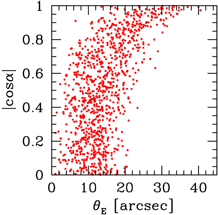
Figure 2: The distribution of the Einstein radii $\theta_{\rm E}$ for 1,000 triaxial haloes with fixed virial mass $M_{\rm vir}=2\times 10^{15}M_{\odot}$. The haloes are located at $z_{l}=0.3$, and the source redshift is assumed to be $z_{s}=1$. The distribution is shown as a function of $|\cos\alpha|$, where $\alpha$ is an angle between the major axis of each halo and the line-of-sight direction. For comparison, the virial radius of the cluster corresponds to $\theta\sim 640^{\prime\prime}$.

To demonstrate the importance of triaxiality on this study, we compute Einstein radii of 1,000 massive dark haloes with the virial mass $M_{\rm vir}=2\times 10^{15}M_{\odot}$ and the redshift $z_{l}=0.3$. The concentration parameter, axis ratios, and the orientation with respect to the line-of-sight direction of each halo are randomly generated using the PDFs described above. We show the resulting distribution of $\theta_{\rm E}$ in Figure 2. The Figure indicates that haloes of the same mass can have a wide range of the Einstein radii. They are correlated with the orientation of the halo such that largest Einstein radii are caused only when the major axis of haloes is almost aligned with the line-of-sight direction ($|\cos\alpha|\sim 1$), implying a strong orientation bias in large lens clusters.

3 Largest Einstein radius and properties of the lensing cluster

3.1 Probability distribution of the largest Einstein radius

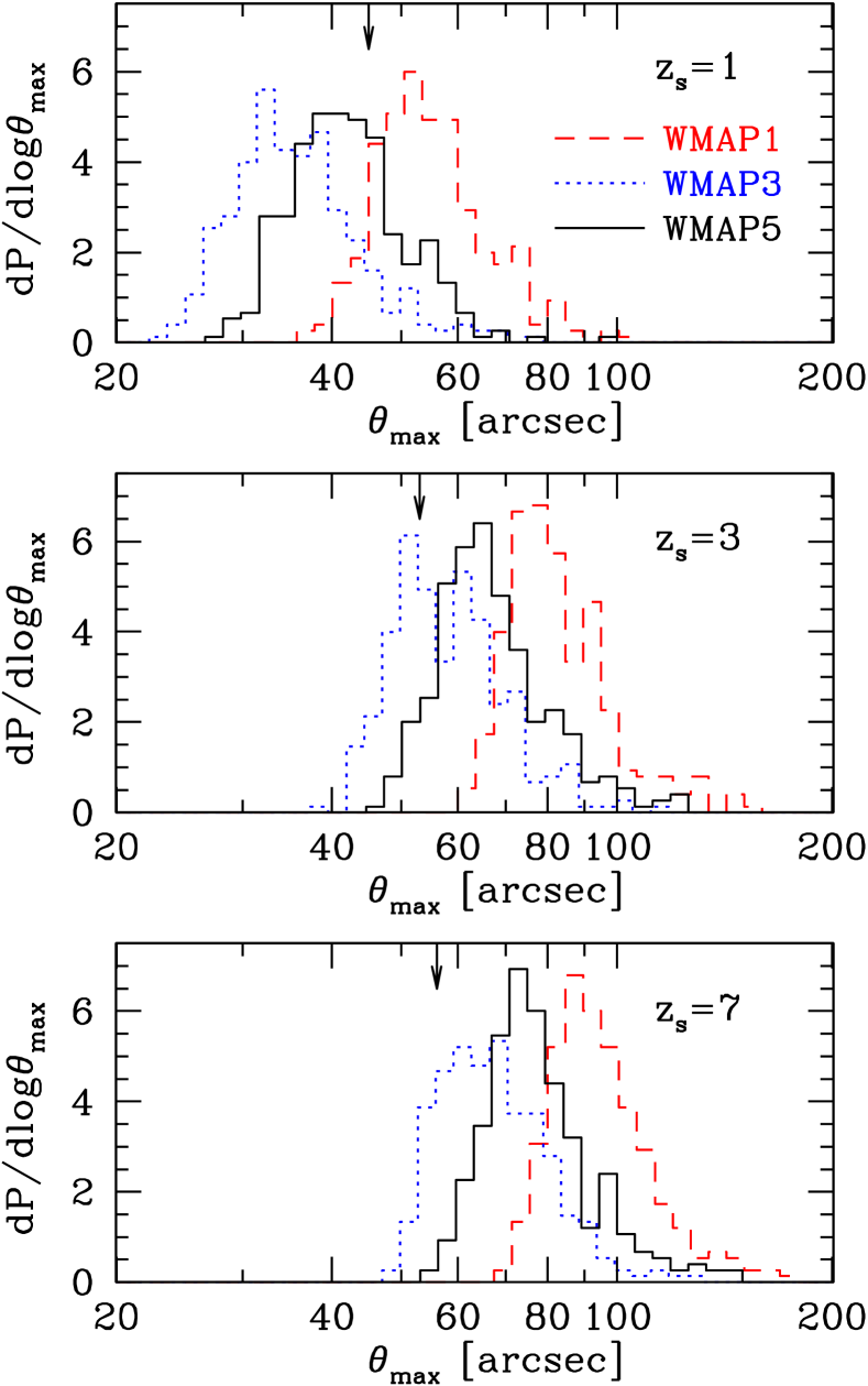
Figure 3: Probability distributions of the largest Einstein radius $\theta_{\rm max}$, constructed from 300 Monte-Carlo realisations of all-sky massive cluster catalogues. From top to bottom panels, source redshifts are assumed to be $z_{s}=1$, $3$, and $7$. Results for three different cosmological models, WMAP1 (dashed), WMAP3 (dotted), and WMAP5 (solid) are shown. Arrows indicate the values of the Einstein radii of A1689, which have the largest known Einstein radii. Note that they correspond to the lower limits of $\theta_{\rm max}$ in observations (see text for details).

First we take the cluster that has the largest Einstein radius from each all-sky realisation. From the 300 realisations for each cosmological model, we can not only construct a probability distribution of the largest Einstein radius in the universe, but also obtain expected properties of the lensing cluster. In what follows, we consider three source redshifts, $z_{s}=1$, $3$, and $7$. The source redshift of $z_{s}=1$ is more relevant to typical giant luminous arcs or weak lensing studies, whereas results for $z_{s}=7$ are more important in searching for high-redshift galaxies near critical curves. The redshift distribution of strongly-lensed faint background galaxies in massive clusters has a peak at $z_{s}\sim 3$ (e.g., Broadhurst et al., 2005b). The probability distributions of the largest Einstein radius in all-sky, $\theta_{\rm max}$, are shown in Figure 3. As expected, $\theta_{\rm max}$ is quite dependent on the cosmological model. For the source redshift $z_{s}=1$, the median of the largest Einstein radius is $\theta_{\rm max}=54^{\prime\prime}$ for WMAP1, $\theta_{\rm max}=35^{\prime\prime}$ for WMAP3, and $\theta_{\rm max}=42^{\prime\prime}$ for WMAP5. The different values of $\sigma_{8}$ ($\sigma_{8}=0.9$ for WMAP1, $\sigma_{8}=0.76$ for WMAP3, and $\sigma_{8}=0.8$ for WMAP5) change the abundance of massive dark haloes and its redshift evolution drastically, which is why the largest Einstein radius is sensitive to $\sigma_{8}$. It is also found that the value of the largest Einstein radius is quite dependent on the source redshift as well: $\theta_{\rm max}$ for $z_{s}=7$ is approximately twice as large as that for $z_{s}=1$.

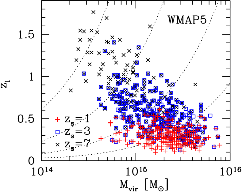
Figure 4: The distribution of the mass and redshift of the cluster producing the largest Einstein radius. Each point corresponds to one Monte-Carlo realisation. Results are shown for three different redshifts, $z_{s}=1$ (pluses), $3$ (open squares), $7$ (crosses). The WMAP5 cosmology is assumed in this plot. Also plotted are contours of constant X-ray fluxes, inferred from the correlation between bolometric X-ray luminosities and halo virial masses (Shimizu et al., 2003, assuming no redshift evolution). From right to left, the contours indicate X-ray fluxes of $f_{X}=10^{-11}$, $10^{-12}$, $10^{-13}$, and $10^{-14}$ ${\rm erg\,s^{-1}cm^{-2}}$.

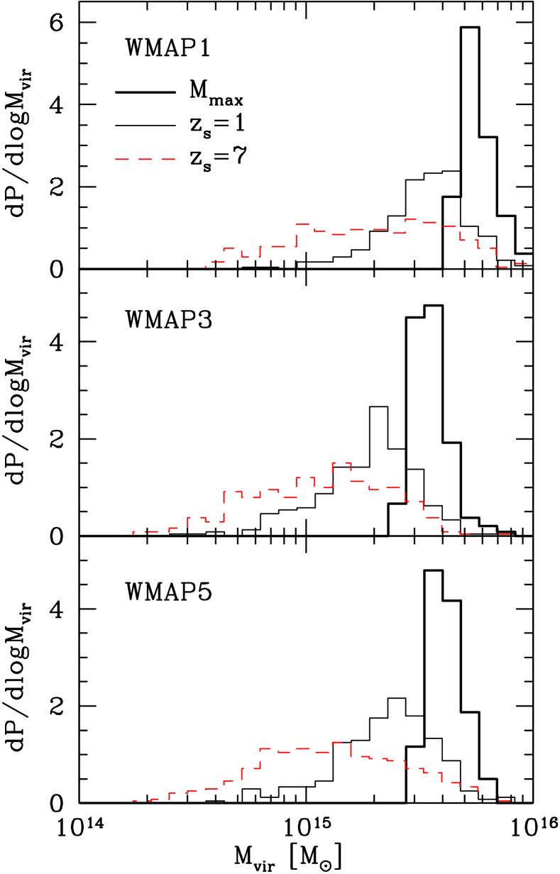
Figure 5: Probability distributions of masses $M_{\rm vir}$ of the most massive cluster in the universe (thick solid) and the cluster producing the largest Einstein radius (thin solid for $z_{s}=1$ and dashed for $z_{s}=7$). From top to bottom panels, we show results for the WMAP1, WMAP3, and WMAP5 cosmologies, respectively.

The cluster which has the largest known Einstein radius to date is A1689. It is a massive cluster located at low redshift ($z_{l}=0.18$), and its Einstein radius is well constrained from many multiply-lensed background galaxies and weak lensing to be $\theta_{\rm E}=45^{\prime\prime}$ for $z_{s}=1$ (Tyson et al., 1990; Miralda-Escudé & Babul, 1995; Clowe & Schneider, 2001; Broadhurst et al., 2005a, b; Umetsu & Broadhurst, 2008). From the best-fit mass model of Umetsu & Broadhurst (2008), we derive $\theta_{\rm E}=53^{\prime\prime}$ for $z_{s}=3$ and $\theta_{\rm E}=56^{\prime\prime}$ for $z_{s}=7$. We emphasise that these values should be viewed as the lower limits of $\theta_{\rm max}$, since even larger lens clusters may be discovered in the future. Nevertheless, we compare these values with our theoretical predictions in Figure 3. For $z_{s}=1$, the Einstein radius of A1689 is quite consistent with our prediction for our fiducial cosmological model, WMAP5. On the other hand it is slightly larger (smaller) than our prediction for WMAP3 (WMAP1), but is within 90 percentile for both WMAP1 and WMAP3. In contrast, the observed values are consistent with WMAP3 and lower than WMAP1 and WMAP5 for $z_{s}=3$. For the higher source redshift $z_{s}=7$, the Einstein radius of A1689 is even smaller than our prediction for WMAP3. An implication of this is that there may exist a cluster with the Einstein radius larger than that of A1689 for that source redshift. We note that cosmological models which predict $\theta_{\rm max}$ close to the Einstein radius of A1689 for $z_{s}=7$, such as models with $\sigma_{8}$ even smaller than WMAP3, should predict too small $\theta_{\rm max}$ for $z_{s}=1$ to be consistent with A1689.

Whilst the better match to WMAP3/WMAP5 is consistent with recent results from the cluster abundance (e.g., Dahle, 2006; Gladders et al., 2007; Mantz et al., 2008), the large discrepancy between the predicted Einstein radii for WMAP1 and those of A1689 does not necessarily exclude WMAP1 cosmology as the current observed $\theta_{\rm max}$ correspond to the lower limits. Complete surveys of large lens clusters are necessary to extract useful cosmological information from this statistics (see §6.1).

3.2 Cluster mass and redshift

Next we examine the expected mass and redshift distribution of the cluster which produces the largest Einstein radii. The distributions shown in Figure 4 indicate that wide ranges of mass and redshift are possible. In particular, it is worth noting that the mass of the cluster can be as small as $M_{\rm vir}<10^{15}M_{\odot}$. In addition, the cluster can be located at quite high-redshifts, up to $z_{l}\sim 1$ and beyond, in the case of $z_{s}=3$ and $7$, which will be difficult to access via X-ray observations with currently operating telescopes (see also discussions in §6.1). On the other hand, for $z_{s}=1$ the lens cluster is likely to be located at $z_{l}<0.5$. Clearly the diversity of the mass and redshift is a consequence of halo triaxiality, which we will explore later.

Here a natural question to ask is whether or not the cluster having the largest Einstein radius is the most massive cluster in the universe. To check this we take the most massive cluster in each realisation and construct the probability distribution of its mass. It is then compared with the PDF of the mass of the largest lens cluster. We show the result in Figure 5. As we discussed, the cluster with $\theta_{\rm max}$ has a wider range of the mass and thus is not necessarily the most massive cluster in the universe. However, the overlap of the PDFs at the high-mass end for all the three cosmological models suggests that in some cases the largest lens corresponds to the most massive cluster. It is interesting to note that the PDFs for $z_{s}=7$ extend to lower masses than those for $z_{s}=1$. This is because the most massive clusters are typically located at $z_{l}\sim 0.1-0.4$, whereas the geometrical lensing efficiency for the source redshift $z_{s}=7$ is the highest at around $z_{l}\sim 1$ where clusters are on average less massive (see also Figure 4).

3.3 Expected properties of the lensing cluster

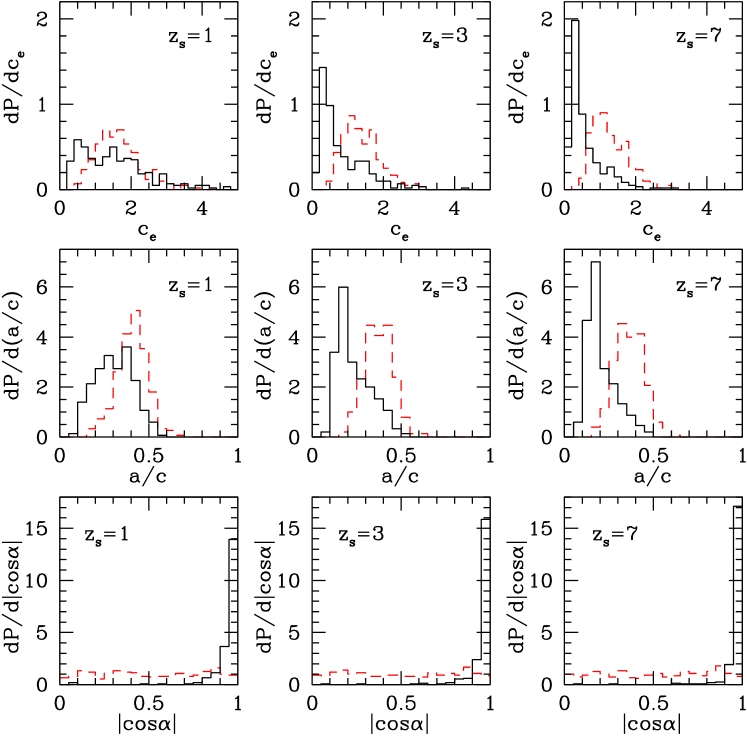
Figure 6: Probability distributions of the triaxial concentration parameter $c_{e}$ (top), the triaxial axis ratio $a/c$ (centre), and the angle between the major axis and the line-of-sight direction $\alpha$ (bottom) for the cluster producing the largest Einstein radius are plotted. For comparison, the PDFs for typical (unbiased) clusters with the same mass and redshift distributions are shown by dashed histograms. From left to right panels, we change the source redshift from $1$ to $7$. Although results shown here are for the WMAP5 cosmology, we confirmed that the PDFs for the other two cosmologies are similar.

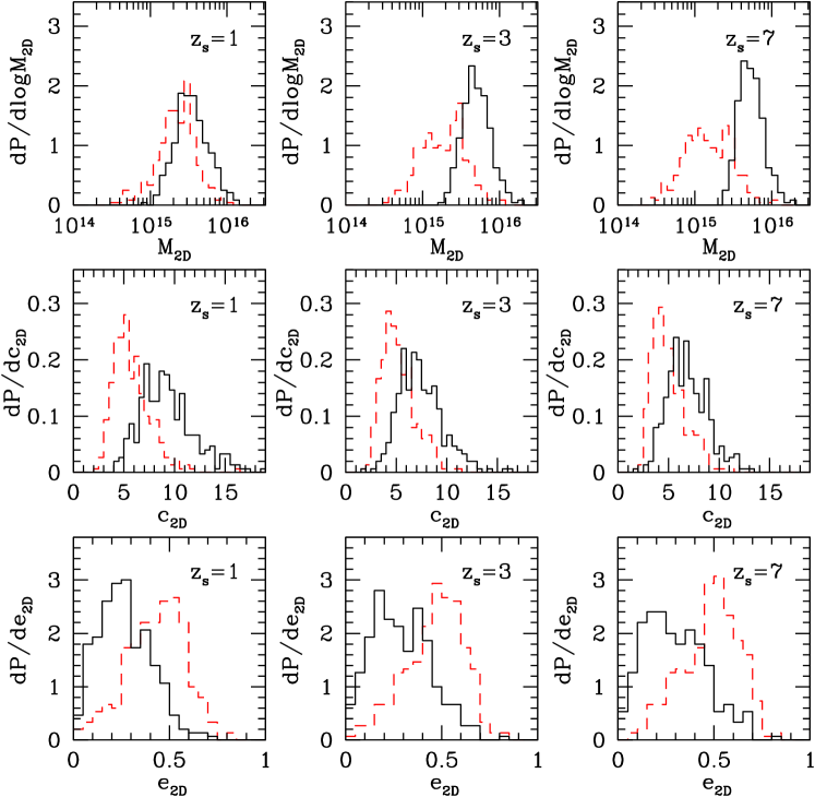
Figure 7: Similar to Figure 6, but the PDFs of the projected two-dimensional virial mass $M_{\rm 2D}$, the projected two-dimensional spherical concentration parameter $c_{\rm 2D}$, and the projected ellipticity $e_{\rm 2D}$ are shown.

Table 1: The largest Einstein radii and expected properties of the lensing clusters. We show median values and 68% confidence intervals estimated from 300 Monte-Carlo realisations. Values in parentheses indicate corresponding parameter values for typical clusters: they are estimated by adopting same mass and redshift distributions as those of the lens cluster and re-assigning concentrations, axis ratios, and orientations according to the PDFs.

Model	$z_{s}$	$\theta_{\rm max}$	$M_{\rm vir}$	$z_{l}$	$c_{e}$	$a/c$	$|\cos\alpha|$	$M_{\rm 2D}$	$c_{\rm 2D}$	$e_{\rm 2D}$
		[arcsec]	[$10^{15}M_{\odot}$]					[$10^{15}M_{\odot}$]
WMAP1	1	$54^{+12}_{-7}$	$3.57^{+1.36}_{-1.32}$	$0.28^{+0.11}_{-0.09}$	$1.57^{+0.98}_{-0.88}$	$0.32^{+0.10}_{-0.10}$	$0.97^{+0.02}_{-0.09}$	$4.58^{+3.03}_{-1.49}$	$8.91^{+2.64}_{-2.11}$	$0.26^{+0.18}_{-0.12}$
					($1.63^{+0.65}_{-0.58}$)	($0.41^{+0.09}_{-0.09}$)	($0.51^{+0.34}_{-0.32}$)	($3.31^{+1.91}_{-1.24}$)	($5.59^{+2.12}_{-1.53}$)	($0.43^{+0.16}_{-0.17}$)
	3	$80^{+15}_{-9}$	$2.83^{+1.87}_{-1.54}$	$0.47^{+0.25}_{-0.17}$	$0.66^{+0.87}_{-0.35}$	$0.23^{+0.11}_{-0.07}$	$0.98^{+0.02}_{-0.06}$	$6.55^{+3.71}_{-1.97}$	$7.03^{+2.27}_{-1.93}$	$0.30^{+0.16}_{-0.15}$
					($1.42^{+0.65}_{-0.46}$)	($0.39^{+0.11}_{-0.09}$)	($0.48^{+0.34}_{-0.34}$)	($2.84^{+1.86}_{-1.46}$)	($5.00^{+2.25}_{-1.22}$)	($0.46^{+0.14}_{-0.18}$)
	7	$92^{+18}_{-10}$	$2.05^{+2.23}_{-1.16}$	$0.62^{+0.35}_{-0.24}$	$0.44^{+0.67}_{-0.20}$	$0.19^{+0.12}_{-0.05}$	$0.98^{+0.02}_{-0.05}$	$7.06^{+3.39}_{-1.77}$	$6.36^{+2.25}_{-1.53}$	$0.33^{+0.16}_{-0.16}$
					($1.29^{+0.60}_{-0.42}$)	($0.39^{+0.08}_{-0.09}$)	($0.48^{+0.38}_{-0.35}$)	($2.26^{+2.37}_{-1.26}$)	($4.88^{+1.66}_{-1.38}$)	($0.48^{+0.14}_{-0.19}$)
WMAP3	1	$35^{+8}_{-6}$	$2.05^{+0.91}_{-0.92}$	$0.29^{+0.13}_{-0.09}$	$1.23^{+1.19}_{-0.76}$	$0.29^{+0.12}_{-0.11}$	$0.98^{+0.02}_{-0.08}$	$2.93^{+2.32}_{-1.07}$	$8.67^{+2.96}_{-2.35}$	$0.26^{+0.18}_{-0.12}$
					($1.52^{+0.64}_{-0.50}$)	($0.40^{+0.09}_{-0.08}$)	($0.54^{+0.29}_{-0.35}$)	($1.95^{+1.29}_{-0.93}$)	($5.37^{+1.91}_{-1.35}$)	($0.45^{+0.15}_{-0.15}$)
	3	$57^{+13}_{-8}$	$1.48^{+1.09}_{-0.77}$	$0.53^{+0.26}_{-0.19}$	$0.57^{+0.66}_{-0.27}$	$0.22^{+0.10}_{-0.07}$	$0.98^{+0.01}_{-0.04}$	$4.18^{+2.05}_{-1.29}$	$6.92^{+2.08}_{-1.60}$	$0.28^{+0.16}_{-0.13}$
					($1.31^{+0.57}_{-0.46}$)	($0.38^{+0.09}_{-0.09}$)	($0.48^{+0.35}_{-0.33}$)	($1.59^{+1.25}_{-0.78}$)	($4.76^{+1.97}_{-1.18}$)	($0.49^{+0.14}_{-0.21}$)
	7	$67^{+13}_{-10}$	$1.23^{+1.23}_{-0.69}$	$0.62^{+0.32}_{-0.23}$	$0.44^{+0.60}_{-0.20}$	$0.19^{+0.11}_{-0.06}$	$0.99^{+0.01}_{-0.04}$	$4.47^{+1.78}_{-1.37}$	$6.65^{+1.94}_{-1.67}$	$0.28^{+0.17}_{-0.13}$
					($1.27^{+0.54}_{-0.43}$)	($0.36^{+0.09}_{-0.07}$)	($0.48^{+0.34}_{-0.31}$)	($1.35^{+1.32}_{-0.73}$)	($4.85^{+1.67}_{-1.30}$)	($0.50^{+0.13}_{-0.17}$)
WMAP5	1	$42^{+9}_{-7}$	$2.35^{+1.21}_{-0.93}$	$0.29^{+0.10}_{-0.10}$	$1.43^{+0.98}_{-0.87}$	$0.31^{+0.11}_{-0.12}$	$0.98^{+0.02}_{-0.06}$	$3.35^{+2.55}_{-1.17}$	$8.99^{+2.78}_{-2.28}$	$0.26^{+0.15}_{-0.13}$
					($1.61^{+0.62}_{-0.55}$)	($0.41^{+0.08}_{-0.09}$)	($0.50^{+0.36}_{-0.33}$)	($2.29^{+1.45}_{-0.98}$)	($5.42^{+2.19}_{-1.31}$)	($0.45^{+0.14}_{-0.17}$)
	3	$65^{+15}_{-8}$	$1.78^{+1.61}_{-0.97}$	$0.52^{+0.23}_{-0.20}$	$0.58^{+0.90}_{-0.29}$	$0.21^{+0.14}_{-0.06}$	$0.98^{+0.01}_{-0.04}$	$4.87^{+2.80}_{-1.55}$	$7.12^{+2.34}_{-1.80}$	$0.28^{+0.17}_{-0.15}$
					($1.31^{+0.56}_{-0.45}$)	($0.37^{+0.08}_{-0.08}$)	($0.50^{+0.36}_{-0.34}$)	($1.94^{+1.55}_{-1.05}$)	($4.97^{+2.03}_{-1.30}$)	($0.49^{+0.12}_{-0.19}$)
	7	$76^{+17}_{-9}$	$1.29^{+1.53}_{-0.67}$	$0.66^{+0.36}_{-0.26}$	$0.41^{+0.66}_{-0.18}$	$0.18^{+0.12}_{-0.04}$	$0.99^{+0.01}_{-0.03}$	$5.15^{+2.65}_{-1.43}$	$6.64^{+2.25}_{-1.73}$	$0.28^{+0.19}_{-0.15}$
					($1.18^{+0.59}_{-0.38}$)	($0.36^{+0.08}_{-0.08}$)	($0.53^{+0.34}_{-0.36}$)	($1.45^{+1.53}_{-0.71}$)	($4.71^{+1.88}_{-1.25}$)	($0.50^{+0.14}_{-0.19}$)

It has been argued that the population of lenses is markedly different from that of nonlenses in several ways (e.g., Oguri et al., 2005b; Hennawi et al., 2007b; Möller et al., 2007; Fedeli et al., 2007; Rozo et al., 2008b). The largest Einstein radius represents the most extreme case of lensing clusters, which suggests that the cluster population may be biased even more strongly. Here we quantify the lensing bias in the cluster producing $\theta_{\rm max}$ from our Monte-Carlo realisations.

As discussed above, an important parameter here is the orientation of the cluster, specifically the angle $\alpha$ between the major axis and the line-of-sight direction. Another important parameter is the minor-to-major axis ratio, $a/c$, since the projection effect is stronger for more triaxial clusters. Finally the concentration parameter of the triaxial model, $c_{e}$, should also be of interest because the strong lensing efficiency is known to be sensitive to the halo concentration.

Figure 6 shows probability distributions of these three parameters for the cluster having $\theta_{\rm max}$. We also show the PDFs for a “typical” cluster which has the same mass and redshift probability distributions as those of the lens cluster but the axis ratio, the concentration, and the orientation are re-assigned from their original PDFs. Thus the comparison of the lens and typical cluster PDFs provides the degree of lensing biases. Strikingly, we find that the cluster is almost always aligned with the line-of-sight direction. For instance, the probability of having $|\cos\alpha|>0.9$ ($\alpha<25.8^{\circ}$) is 0.88 for $z_{s}=1$ and 0.95 for $z_{s}=7$ for the WMAP5 cosmology. It is also found that the lens cluster is more triaxial than typical clusters. Because of the correlation between $c_{e}$ and $a/c$, the triaxial concentration parameter for the lens cluster becomes smaller. The strong biases in the orientation and triaxiality indicate that such largest lens cluster is indeed very unusual in terms of its internal structure and configuration.

The projection effect of the triaxial halo has a large impact on the apparent mass profile constrained from lensing data (Oguri et al., 2005a). To investigate this, we characterise the projected two-dimensional (2D) mass distribution of each triaxial cluster by the following three parameters: the mass $M_{\rm 2D}$ and concentration parameter $c_{\rm 2D}$ of the NFW profile, which are obtained from the projected surface mass density by ignoring the elongation along the line-of-sight, and the ellipticity of the surface mass density $e_{\rm 2D}$. Our parameter $c_{\rm 2D}$ corresponds to the standard concentration parameter which has been studied from analysis of observed lensing clusters, and thus is useful for discussing possible high concentrations from lens mass reconstructions (e.g., Broadhurst et al., 2005a). We can relate these parameters to those of the triaxial halo by simply comparing the expressions of the projected surface mass densities (K. Takahashi et al., in preparation):

$$1-e_{\rm 2D}=q,$$ (19)

$$\frac{r_{\rm vir}(M_{\rm 2D})}{\sqrt{q}c_{\rm 2D}}=R_{0}q_{x},$$ (20)

$$b_{\rm NFW}(M_{\rm 2D},c_{\rm 2D})=b_{\rm TNFW}(M_{\rm vir},c_{e}),$$ (21)

where $b_{\rm NFW}$ is the lensing strength parameter for the spherical NFW profile.

We show probability distributions of these 2D parameters, for both the cluster having $\theta_{\rm max}$ and corresponding typical cluster, in Figure 7. It is clear that the largest lens cluster is highly biased in terms of the 2D parameters as well. In lensing observations the lens cluster looks more massive and more centrally concentrated than typical clusters. Indeed this is expected from the strong orientation bias (see above), because both the mass and concentration of the cluster projected along the major axis are known to be significantly overestimated (Oguri et al., 2005a; Corless & King, 2008). In addition we find that the cluster should appear rounder. Its expected median ellipticity of $0.25-0.3$ is significantly smaller than that of typical triaxial cluster, $0.45-0.5$. Again, this is because of the orientation bias: the projected mass distribution of a triaxial halo is most elliptical when it is projected along the middle axis, and least elliptical when projected along major or minor axis. This means that the circularity of projected density distribution do not necessarily imply the sphericity of the cluster. We summarise our numerical results in Table 1.

We are now in a position of discussing the high concentration parameters observed in some lens-rich clusters. For instance, from the strong and weak lensing data Umetsu & Broadhurst (2008) refined the concentration parameter of A1689, which has the largest known Einstein radius, to be $c_{\rm 2D}=12.7$ assuming a spherical NFW profile. Adopting the source redshift $z_{s}=1$, our model predicts that such a cluster should have the concentration parameter in the range $6.7<c_{\rm 2D}<11.8$ at 68% confidence and $5.5<c_{\rm 2D}<14.8$ at 90% confidence. Thus we conclude that the high concentration of A1689 is consistent with the theoretical expectation based on the F$\Lambda$CDM model at $1.2\sigma$ level. We note that the redshift of the cluster is also consistent at $\sim 1\sigma$ level. However the halo concentration of A1689 is still slightly larger than the theoretical expectation. Therefore statistical studies of concentrations for several large lens clusters, as attempted in Broadhurst & Barkana (2008) and Broadhurst et al. (2008), will be essential to assess whether or not the large concentration problem is indeed existent.

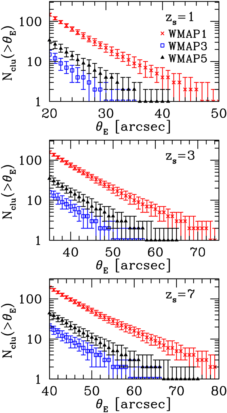
Figure 8: Expected all-sky cumulative number distributions of large Einstein radii. The median and $1\sigma$ error-bars of the numbers are estimated from 300 Monte-Carlo realisations. Results are presented for all the three cosmological models, WMAP1 (crosses), WMAP3 (squares), and WMAP5 (triangles). From top to bottom panels, results for $z_{s}=1$, $3$, and $7$ are shown.

4 Distribution of Einstein radii

Thus far we focused our attention on the largest Einstein radius on the sky. Another interesting quantity to investigate is the number of clusters which have relatively large Einstein radii. Here we derive the expected number distribution of such large Einstein radii from our Monte-Carlo realisations.

In Figure 8, we plot the cumulative number distributions for all the three cosmological models. It is found that the number decreases exponentially with increasing Einstein radius. As in the case of the largest Einstein radius, the abundance of large lens clusters is quite sensitive to the cosmological model. For instance, the all-sky numbers of clusters which have $\theta_{\rm E}>20^{\prime\prime}$ (for $z_{s}=1$) are predicted to be $\sim 150$, $\sim 15$, $\sim 35$, for WMAP1, WMAP3, and WMAP5 cosmologies, respectively. The large difference of the cumulative numbers between WMAP1 and WMAP3 is broadly consistent with Li et al. (2006, 2007) who investigated strong lensing probabilities in two different cosmological simulations. The result suggests that it provides useful constraints on cosmological parameters.

One of the main findings about the largest Einstein radius was that the lens clusters constitute a highly biased population (see Section 3.3). One might expect that the strong bias is due to the rareness of such largest lens, and thus it is interesting to check lensing biases for more common lens events. In Figure 9, we show biases in clusters which have Einstein radii larger than certain values. Here we adopt two parameters to quantify lensing biases. One is a measure of the orientation bias, $f_{|\cos\alpha>0.9|}$, which is defined by the fraction that the angle between the major axis of the cluster and the line-of-sight direction satisfies $|\cos\alpha|>0.9$. If the orientation of clusters is completely random, we should have $f_{|\cos\alpha>0.9|}\approx 0.1$. The other parameter is to describe the 2D concentration bias, $\overline{c_{\rm 2D}}/\overline{c_{\rm 2D,ran}}$, which is the ratio of median 2D concentration parameters (see also Section 3.3) among large lens clusters and corresponding typical clusters with similar mass and redshift distributions. The parameter becomes unity if no lensing bias is present.

The result shown in Figure 9 indicates that clusters with large Einstein radii are similarly highly biased as the cluster producing the largest Einstein radii in all-sky. We find that the degree of the orientation bias depends on the limiting Einstein radius. Populations of clusters with smaller limiting Einstein radius, which are regarded to represent less extreme populations of lensing clusters, are less biased in terms of their orientations. On the other hand, the degree of the 2D concentration bias does not depend strongly on the limiting Einstein radius. The bias in the 2D concentration parameter comes both from the enhancement of the apparent concentration due to the orientation bias and from the bias in the 3D triaxial concentration parameter. The enhancement of $c_{\rm 2D}$ due to the orientation bias is larger for more triaxial haloes, however because of the anti-correlation between the axis ratio and concentration (Jing & Suto, 2002) such haloes are intrinsically less concentrated (i.e., have smaller $c_{e}$). The behavior is therefore expected to reflect the complicated combination of these two biases which are more or less counteract with each other.

Our results can be compared with those of Hennawi et al. (2007b) who analysed lensing biases using ray-tracing of $N$-body simulations. Their qualitative results are similar to ours: they found that lensing clusters tend to have the major axis aligned with the line-of-sight and larger 2D concentrations. However, the quantitative results are different. Their orientation bias of $f_{|\cos\alpha>0.9|}\sim 0.25$ and 2D concentration bias of $\overline{c_{\rm 2D}}/\overline{c_{\rm 2D,ran}}\sim 1.34$ are smaller than our results (see Figure 9). We ascribe this difference to the different definitions of the lens cluster populations. Hennawi et al. (2007b) derived the distributions for lens clusters by calculating those from all clusters with a weight of lensing cross sections, without any restriction to the Einstein radii. Therefore their results are relevant to more common lens clusters with smaller Einstein radii, say $10^{\prime\prime}-15^{\prime\prime}$, whereas our results are applicable only to superlens clusters with unusually large Einstein radii. Our finding that the orientation bias decreases with decreasing Einstein radius is consistent with this interpretation.

5 Primordial Non-Gaussianity

The results presented so far are based on standard universes evolved from Gaussian initial conditions. Since the abundance of massive clusters and its redshift evolution are known to be very sensitive to primordial non-Gaussianities (e.g., Matarrese et al., 2000; Verde et al., 2001; Mathis et al., 2004; Grossi et al., 2007; Sadeh et al., 2007; Fedeli et al., 2008; Dalal et al., 2008), our statistics are also expected to be dependent on primordial non-Gaussianities. The effect of primordial non-Gaussianities is particularly of importance given possible detections in the cosmic microwave background (CMB) anisotropies (e.g., Vielva et al., 2004; Yadav & Wandelt, 2008). In this section, we repeat the same calculations conducted in the previous sections, but including levels of primordial non-Gaussianities currently of interest.

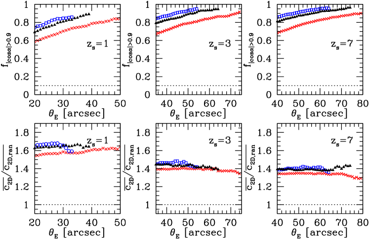
Figure 9: The dependence of lensing biases on the limiting Einstein radius $\theta_{\rm E}$. Each point shows lensing biases of the cluster orientation (upper), $f_{|\cos\alpha>0.9|}$, or that of the concentration parameter inferred from the projected 2D mass distribution (lower), $\overline{c_{\rm 2D}}/\overline{c_{\rm 2D,ran}}$, in clusters having the Einstein radii larger than $\theta_{\rm E}$. See text for the definitions of these parameters. Horizontal dotted lines indicate values in the case with no bias. Crosses, open squares, and filled triangles denote results for WMAP1, WMAP3, and WMAP5 models, respectively. We consider the source redshift of $z_{s}=1$ (left), $3$ (centre), and $7$ (right).

In order to quantify the effect of primordial non-Gaussianities, in this paper we adopt the local non-Gaussianity of the following form (e.g., Komatsu & Spergel, 2001; Bartolo et al., 2004):

$$\Phi=\phi+f_{\rm NL}\left(\phi^{2}-\langle\phi^{2}\rangle\right),$$ (22)

where $\Phi$ is the curvature perturbation and $\phi$ is an auxiliary random-Gaussian field. The level of primordial non-Gaussianity is characterised by $f_{\rm NL}$, which we assume constant. In this model positive $f_{\rm NL}$ corresponds to positive skewness of the density field. In observation, CMB anisotropies have constrained its value to be $|f_{\rm NL}|\la\mathcal{O}(100)$. For instance, Komatsu et al. (2003) derived $-58<f_{\rm NL}<134$ at 95% confidence from the temperature map of the WMAP first-year data. More recently, Yadav & Wandelt (2008) claimed the detection of positive $f_{\rm NL}$, $26.9<f_{\rm NL}<146.7$ at 95% confidence, from the improved analysis of the WMAP three-year data. On the other hand, Komatsu et al. (2008) claimed that the WMAP five-year data are marginally consistent with Gaussian fluctuations at 95% confidence, $-9<f_{\rm NL}<111$.

We follow Dalal et al. (2008) to calculate the number of massive haloes in this non-Gaussian model. From analytic considerations and $N$-body simulations, they derived a simple fitting formula of the mass function:

$$\frac{dn_{\rm NG}}{dM}=\int\frac{dM_{0}}{M_{0}}\frac{dn}{dM_{0}}\frac{1}{\sqrt{2\pi}\sigma_{f}}\exp\left[-\frac{(M/M_{0}-f_{M})^{2}}{2\sigma_{f}^{2}}\right],$$ (23)

where $dn/dM_{0}$ is a halo mass function with a Gaussian initial condition, which we adopt equation (1), and

$$f_{M}=1+1.3\times 10^{-4}f_{\rm NL}\sigma_{8}\sigma_{M_{0}}^{-2},$$ (24)

$$\sigma_{f}=1.4\times 10^{-4}(|f_{\rm NL}|\sigma_{8})^{0.8}\sigma_{M_{0}}^{-1}.$$ (25)

From this expression, we can see that the positive $f_{\rm NL}$ results in the enhancement of the abundance of massive clusters.

Primordial non-Gaussianities affect not only the abundance of massive clusters but also their formation histories. Since the concentrations of dark haloes are correlated with their mass assembly histories (Wechsler et al., 2002), primordial non-Gaussianities should have an impact on the halo concentration parameter as well. Indeed, $N$-body simulations done by Avila-Reese et al. (2003) showed that positive (negative) skewness in the initial density field results in larger (smaller) halo concentrations. We crudely include this effect by modifying the linear overdensity in equation (12) as follows (Matarrese et al., 2000):

$$\delta_{c}(z)\rightarrow\delta_{c}(z)\sqrt{1-S_{3}\delta_{c}(z)/3}.$$ (26)

We estimate the skewness $S_{3}$ as $S_{3}\sim 6f_{\rm NL}\sigma_{M}^{-1}\sigma_{\phi}$ with $\sigma_{\phi}=4\times 10^{-5}$ (Dalal et al., 2008). In this model, primordial non-Gaussianity of $f_{\rm NL}=\pm 200$ translates into the modification of median concentration parameters for haloes with the mass $10^{15}M_{\odot}$ by $\sim\pm 5\%$. Given the current level of constraints on $f_{\rm NL}$ from WMAP (e.g., Komatsu et al., 2003; Spergel et al., 2007; Yadav & Wandelt, 2008; Hikage et al., 2008), in this section we consider three non-Gaussian models, $f_{\rm NL}=-100$, $100$, and $200$, as well as the Gaussian case $f_{\rm NL}=0$ studied in the previous sections. For each model, we compute 300 realisations of all-sky cluster catalogue to estimate median and cosmic variance of large lenses. First, we examine the effect of primordial non-Gaussianities on the probability distribution of the largest Einstein radii $\theta_{\rm max}$. The dependence of $\theta_{\rm max}$ on $f_{\rm NL}$ is displayed in Figure 10. We find that primordial non-Gaussianity of $|f_{\rm NL}|\sim 100$ hardly affect $\theta_{\rm max}$. Although $\theta_{\rm max}$ is increased by $\sim 10\%$ from $f_{\rm NL}=-100$ to $200$, it is clearly smaller than the cosmic variance. This suggests that the observation of $\theta_{\rm max}$ hardly constrains $f_{\rm NL}$, at least not so tightly as the current WMAP data do. On the other hand, the plot shown in Figure 11 suggests that we can in principle detect primordial non-Gaussianities of $|f_{\rm NL}|\sim 100$ from the all-sky abundance of clusters with relatively large Einstein radii, $N(>\theta_{\rm E})$. For instance, $N(>20^{\prime\prime})$ for $z_{s}=1$ is $34\pm 6$ and $60^{+10}_{-8}$ (68% confidence) for $f_{\rm NL}=0$ and $200$, respectively. The abundances of large lenses for higher source redshifts are more sensitive to $f_{\rm NL}$, because lens clusters are located at higher redshifts where the cluster abundance is more sensitive to primordial non-Gaussianities. One of the reasons why the abundance of large Einstein radii is better in probing $f_{\rm NL}$ than the observation of $\theta_{\rm max}$ is its smaller cosmic variance.

Figure 10: The largest Einstein radius in all-sky as a function of primordial non-Gaussianities $f_{\rm NL}$. WMAP5 cosmology is assumed. The error-bars show 68% confidence estimated from 300 Monte-Carlo realisations. The source redshifts are assumed to be $z_{s}=1$, $3$, and $7$ from top to bottom panels.

Figure 11: Similar to Figure 10, but the numbers of clusters with the Einstein radii larger than certain values are plotted. The limiting Einstein radii are $20^{\prime\prime}$ ($z_{s}=1$), $35^{\prime\prime}$ ($z_{s}=3$), and $40^{\prime\prime}$ ($z_{s}=7$).

The results presented above suggest that constraints on $f_{\rm NL}$ are not improved very much by including large lenses, compared with current CMB constraints. However, some inflation models predict strongly scale-dependent primordial non-Gaussianities (e.g., LoVerde et al., 2008), and thus independent constraints from clusters of galaxies, which probe smaller scales (a few Mpc) than CMB anisotropies ($\ga 100$ Mpc), can be very important to test such scale-dependence. The best constraints on primordial non-Gaussianities at the cluster scale are expected to be obtained by the number count of clusters at high-redshifts, detected in radio, X-ray, or optical, but an accurate calibration of cluster masses is always challenging (e.g., Hu et al., 2007; Takada & Bridle, 2007). The statistics of large lenses may therefore provide an important complementary test of cluster-scale primordial non-Gaussianities.

6 Discussions

6.1 Observational strategy

In this paper, we derived all-sky distributions of large Einstein radii based on the F$\Lambda$CDM model. An advantage of the Einstein radius statistics is that it is determined quite well from observations, provided that strongly lensed arcs are observed. How many arcs do we expect? Oguri et al. (2003) computed the number of lensed arcs in a typical massive cluster, with a mass of $2-3\times 10^{15}M_{\odot}$, to be $\sim 1$ for the arc magnitude limit of $\sim 26$ mag. Since the clusters studied in this paper have $2-3$ times larger Einstein radius than typical clusters of similar masses, the expected number of lensed arcs for these clusters should also be larger by a factor of $5-10$. Therefore, we conclude that reasonably deep ($\sim 26$ mag) optical imaging of clusters having large Einstein radii should always reveal several strongly lensed arcs, which will be sufficient to determine their critical curves accurately. This is indeed the case in the largest known lens clusters such as A1689 (Broadhurst et al., 2005b), CL0024+1654 (Kneib et al., 2003; Jee et al., 2007), RXJ1347$-$1145 (Bradač et al., 2005, 2008; Halkola et al., 2008), SDSS J1209+2640 (Ofek et al., 2008), and RCS2 2327$-$02 (M. Gladders et al., in preparation) in which many strong lensing events are already identified.

The discussion above suggests that wide-field deep optical surveys, such as done by the Large Synoptic Survey Telescope (LSST; Ivezic et al., 2008), provide a promising way to locate clusters with very large Einstein radii. In such optical surveys, we will be able to search for strongly lensed arcs directly without a priori information on locations of massive clusters (e.g., Horesh et al., 2005; Seidel & Bartelmann, 2007). Such blind/automated arc survey has been attempted by Cabanac et al. (2007) using Canada-France-Hawaii Telescope Legacy Survey (CFHTLS) data. The detection and characterisation of massive clusters using weak lensing (e.g., Miyazaki et al., 2007) will complement the identifications of lensed arcs and will allow a check of the model of clusters that we adopted in Section 2. Another approach is to make use of (shallower) optical, X-ray, or Sunyaev-Zel’dovich (SZ) surveys to identify candidate massive clusters, and conduct follow-up optical imaging of each massive cluster to characterise its lensing properties. Examples of such optical/X-ray/SZ cluster surveys include the maxBCG cluster survey (Koester et al., 2007), the ROSAT-ESO Flux Limited X-ray (REFLEX) Galaxy cluster survey (Böhringer et al., 2004), the Massive Cluster Survey (MACS; Ebeling et al., 2007), the ROSAT PSPC Galaxy Cluster Survey (Burenin et al., 2007), the Red-Sequence Cluster Survey (RCS; Gladders & Yee, 2005), and planned SZ cluster surveys such as the South Pole Telescope (SPT), the Atacama Cosmology Telescope (ACT), the Atacama Pathfinder EXperiment (APEX) SZ survey, and a survey using the Planck satellite. However, clusters with largest Einstein radii are not necessarily the most massive. Cluster surveys need to be deep enough to locate masses as small as $\sim 5\times 10^{14}M_{\odot}$ to assure completeness (see also Figure 4).

The critical curves of the largest lenses predicted in our model may offer guidance for identifying such systems in observations. In Figure 12, we plot our prediction for the plausible critical curves of the largest lens, as well as the critical curves of A1689 obtained in Broadhurst et al. (2005b). Because of the high concentration and rounder shape of the projected mass distribution, the predicted inner critical curves are rather small compared with the outer critical curve. Therefore for these systems strong lens events are dominated by standard “double” and “quadruple” image configurations. This is in marked contrast to typical clusters in which less concentrated 2D mass distributions increase the importance of their inner critical curves and produce naked cusp image configurations (e.g, Blandford & Kochanek, 1987; Oguri & Keeton, 2004; Oguri et al., 2008). We find that the critical curves of the largest known lens cluster A1689 are similar despite the perturbation by several substructures.

Figure 12: Critical curves of A1689 ($z_{s}=3$) constrained from multiple strong lens systems (Broadhurst et al., 2005b) are compared with the most plausible critical curves of the largest lens in our model, which is obtained from the median parameter values listed Table 1.

One of our main findings is that large lens clusters represent a highly biased population. Whilst the biases in projected 2D mass distributions can directly be tested from lensing observations of clusters, the alignment between major axes and line-of-sight directions will require additional observations. For instance, the line-of-sight elongation of a cluster can be inferred by combining multi-wavelength data such as X-ray, SZ, and kinematics of member galaxies (e.g., Fox & Pen, 2002; Lee & Suto, 2004; Gavazzi, 2005; Sereno, 2007; Ameglio et al., 2007).

6.2 Effect of baryons

The triaxial halo model of JS02, which we adopted, is based on $N$-body simulations of dark matter. It is of interest to see how baryon physics can affect our results. The most important baryonic effect on cluster strong lensing comes from the central galaxy (e.g., Meneghetti et al., 2003b; Sand et al., 2005; Puchwein et al., 2005; Hennawi et al., 2007b; Rozo et al., 2008a; Wambsganss et al., 2008; Hilbert et al., 2008). Although the central galaxy can boost the lensing probability as high as $\sim 100\%$, the effect is clearly scale dependent such that clusters with smaller Einstein radii are more substantially affected by central galaxies. Both analytic and numerical studies agree in that for lensing with large Einstein radii ($\theta_{\rm E}\ga 20^{\prime\prime}$) the enhancement of lensing probabilities due to central galaxies become negligibly small (see, e.g., Oguri, 2006; Wambsganss et al., 2008; Hilbert et al., 2008; Minor & Kaplinghat, 2008), suggesting that the clusters discussed in this paper, which have unusually large Einstein radii, are not affected by central galaxies. This is also expected from the fact that their critical curves extend far beyond central galaxies. Therefore we conclude that the effect of central galaxies is negligibly small for our results.

Baryons also influence the shape of clusters. For instance, dissipative gas cooling results in more spherical dark haloes (Kazantzidis et al., 2004). In addition, the inclusion of hot gas components slightly enhances the concentration of dark haloes (Rasia et al., 2004; Lin et al., 2006), although current studies are insufficient to quantify its statistical impact.

6.3 Other possible systematics

Cluster substructures affect the shapes and locations of arcs and hence may influence the Einstein radius. However, Meneghetti et al. (2007) found that the radial shift due to substructures is $\la 5^{\prime\prime}$ (see also Peirani et al., 2008), much less than $\theta_{\rm E}$ considered in this paper, and the effect cancels out to first order.

Some clusters have quite complicated morphology which cannot be described by a simple ellipsoid. An extreme example is the merger as seen in the bullet cluster (Clowe et al., 2006), which turned out to have a large impact on arc statistics (Torri et al., 2004). One of the reasons for the large effect of mergers on arc cross sections is that complicated mass distributions tend to induce many cusps in caustics where prominent, long and thin arcs are preferentially formed. In contrast, the size of the Einstein radius is simply determined by the mass it encloses, and therefore the Einstein radius should be less sensitive to the complexity of the mass distribution. In addition, clusters which undergo merger events can be represented approximately by triaxial haloes with very small axis ratios $a/c$. In this sense our calculation includes the effect of mergers. The more robust treatment of mergers will require calibration using high-resolution $N$-body simulations.

In our calculations we have ignored any chance projection of multiple clusters along the line-of-sight. We make a rough estimate for the expected number of such events as follows. We consider following two situations: (1) superposition of two massive haloes, and (2) a small halo on top of a massive halo. For case (1), we require that both haloes should have masses $M>7\times 10^{14}M_{\odot}$, because the superposition of two clusters with these masses result in the total Einstein radius of the system large enough to affect our results ($\theta_{\rm E}\ga 30^{\prime\prime}$ for $z_{s}=3$). From the all-sky number of such clusters, $N_{\rm clu}\approx 4,400$ for WMAP5, we compute the chance probability as $N_{\rm clu}^{2}\Omega^{-1}\pi\theta^{2}[1+\omega(\theta)]\approx 0.1\times[1+\omega(\theta)]\la 1$ (e.g., Brodwin et al., 2007, for the angular correlation function $\omega(\theta)$), much smaller than the predicted abundance of large lenses (e.g., $N(>35^{\prime\prime})\approx 35$ for $z_{s}=3$). For case (2), we consider superpositions of massive haloes with $M>1\times 10^{15}M_{\odot}$ and smaller haloes with $M>1\times 10^{14}M_{\odot}$ from the same reason, i.e., the superposition of these haloes with typical concentrations yields the total Einstein radius with its size comparable to that discussed in the paper. The all-sky numbers, $1,100$ and $86,000$ respectively, suggest the chance probability of $\approx 0.5\times[1+\omega(\theta)]\la 1$, again smaller compared with the predicted abundance of superlenses. Thus we expect that the effect of the chance projection of multiple clusters is not significant.

However, it has been argued that A1689 may have a possible secondary peak along line-of-sight (Andersson & Madejski, 2004; Łokas et al., 2006; King & Corless, 2007), which implies that multiple clusters might in practice have some impact on the statistics of superlenses. Ray-tracing in large-box $N$-body simulations should provide an important cross-check of how important projections of haloes along line-of-sight are.

7 Conclusion

We have calculated the expected distributions of large Einstein radii in all-sky (40,000 ${\rm deg^{2}}$) using a triaxial halo model. Our approach to generate all-sky mock catalogue of massive clusters and the properties of individual clusters with the Monte-Carlo method allows us to evaluate the cosmic variance for such statistics, and at the same time, to study biases in the population of clusters having such large Einstein radii.

The largest Einstein radius in all-sky for source redshift $z_{s}=1$ was predicted to be $42{}^{+9}_{-7}$ arcseconds for WMAP5, $35{}^{+8}_{-6}$ arcseconds for WMAP3, and $54{}^{+12}_{-7}$ arcseconds for WMAP1, where errors are $1\sigma$ cosmic variance. The sensitivity to $\sigma_{8}$ suggests that this statistic is a good measure of it. The Einstein radii are approximately twice as large for larger source redshift, $z_{s}=7$. In some realisations the largest lens cluster is the most massive cluster in the universe; in others smaller than $10^{15}M_{\odot}$. We have found that the population of these “superlens” clusters are significantly biased: their major axes are almost always aligned with the line-of-sight, and their projected 2D mass distributions appear rounder (by $\Delta e\sim 0.2$) and more concentrated ($\sim 40-60\%$ larger values of concentration parameters). These biases are stronger than those found in more common lens clusters with smaller Einstein radii (Hennawi et al., 2007b). In particular we have pointed out that the high concentration observed in A1689 is consistent with our theoretical expectation at the $1.2\sigma$ level. Thus the combined analysis of several clusters will be essential to address the claimed high concentration problem. Finally, we have studied the effect of primordial non-Gaussianities, and concluded that the abundance of relatively large lens clusters can in principle constrain primordial non-Gaussianities at a level comparable to the current CMB experiments ($|f_{\rm NL}|\sim 100$), if other cosmological parameters are fixed.

It will be very important to compare our analytic predictions with ray-tracing in $N$-body simulations. In particular, the large cosmological Millennium Simulation (Springel et al., 2005) has sufficient resolution to resolve the centres of massive dark haloes for strong lensing studies (Hilbert et al., 2007, 2008). Although its small box size ($500h^{-1}{\rm Mpc}$) does not allow predictions for all-sky distributions of Einstein radii, we can use these simulations to validate and calibrate our semi-analytical model predictions. The comparison of our results with those from $N$-body simulations will be presented in a forthcoming paper.

The statistics of large Einstein radii provide an important opportunity to test the standard F$\Lambda$CDM paradigm, as it probes both the high-mass end of the cluster mass function and central mass distributions of massive clusters. The measurement of Einstein radii is fairly robust, and future all-sky samples will soon be available to perform this study.

References

- Allgood et al. (2006) Allgood B., Flores R. A., Primack J. R., Kravtsov A. V., Wechsler R. H., Faltenbacher A., Bullock J. S., 2006, MNRAS, 367, 1781
- Ameglio et al. (2007) Ameglio S., Borgani S., Pierpaoli E., Dolag K., 2007, MNRAS, 382, 397
- Andersson & Madejski (2004) Andersson K. E., Madejski G. M., 2004, ApJ, 607, 190
- Avila-Reese et al. (2003) Avila-Reese V., Colín P., Piccinelli G., Firmani C., 2003, ApJ, 598, 36
- Baltz et al. (2008) Baltz E. A., Marshall P., Oguri M., 2008, arXiv:0705.0682
- Bartelmann et al. (1998) Bartelmann M., Huss A., Colberg J. M., Jenkins A., Pearce F. R., 1998, A&A, 330, 1
- Bartelmann et al. (1995) Bartelmann M., Steinmetz M., Weiss A., 1995, A&A, 297, 1
- Bartolo et al. (2004) Bartolo N., Komatsu E., Matarrese S., Riotto A., 2004, PhR, 402, 103
- Blandford & Kochanek (1987) Blandford R. D., Kochanek C. S., 1987, ApJ, 321, 658
- Böhringer et al. (2004) Böhringer H., et al., 2004, A&A, 425, 367
- Bouwens et al. (2008) Bouwens R. J., et al., 2008, ApJ, submitted (arXiv:0805.0593)
- Bradač et al. (2005) Bradač M., et al., 2005, A&A, 437, 49
- Bradač et al. (2008) Bradač M., et al., 2008, ApJ, 681, 187
- Broadhurst & Barkana (2008) Broadhurst T., Barkana R., 2008, MNRAS, in press (arXiv:0801.1875)
- Broadhurst et al. (2005a) Broadhurst T., Takada M., Umetsu K., Kong X., Arimoto N., Chiba M., Futamase T., 2005a, ApJ, 619, L143
- Broadhurst et al. (2005b) Broadhurst T., et al., 2005b, ApJ, 621, 53
- Broadhurst et al. (2008) Broadhurst T., Umetsu K., Medezinski E., Oguri M., Rephaeli Y., 2008, ApJ, 685, L9
- Brodwin et al. (2007) Brodwin M., Gonzalez A. H., Moustakas L. A., Eisenhardt P. R., Stanford S. A., Stern D., Brown M. J. I., 2007, ApJ, 671, L93
- Burenin et al. (2007) Burenin R. A., Vikhlinin A., Hornstrup A., Ebeling H., Quintana H., Mescheryakov A., 2007, ApJS, 172, 561
- Cabanac et al. (2007) Cabanac R. A., et al., 2007, A&A, 461, 813
- Chen (2004) Chen D.-M., 2004, A&A, 418, 387
- Chen (2005) Chen D.-M., 2005, ApJ, 629, 23
- Clowe & Schneider (2001) Clowe D., Schneider P., 2001, A&A, 379, 384
- Clowe et al. (2006) Clowe D., Bradač M., Gonzalez A. H., Markevitch M., Randall S. W., Jones C., Zaritsky D., 2006, ApJ, 648, L109
- Comerford & Natarajan (2007) Comerford J. M., Natarajan P., 2007, MNRAS, 379, 190
- Cooray (1999) Cooray A. R., 1999, A&A, 341, 653
- Corless & King (2007) Corless V. L., King L. J., 2007, MNRAS, 380, 149
- Corless & King (2008) Corless V. L., King L. J., 2008, MNRAS, in press (arXiv:0807.4642)
- Dahle (2006) Dahle H., 2006, ApJ, 653, 954
- Dalal et al. (2008) Dalal N., Doré O., Huterer D., Shirokov A., 2008, PhRvD, 77, 123514
- Dalal et al. (2004) Dalal N., Holder G., Hennawi J. F., 2004, ApJ, 609, 50
- Duffy et al. (2008) Duffy A. R., Schaye J., Kay S. T., Dalla Vecchia C., 2008, MNRAS, 390, L64
- Dunkley et al. (2008) Dunkley J., et al., 2008, ApJS, in press (arXiv:0803.0586)
- Ebeling et al. (2007) Ebeling H., Barrett E., Donovan D., Ma C.-J., Edge A. C., van Speybroeck L., 2007, ApJ, 661, L33
- Eisenstein & Hu (1998) Eisenstein D. J., Hu W., 1998, ApJ, 496, 605
- Ellis et al. (2001) Ellis R., Santos M. R., Kneib J.-P., Kuijken K., 2001, ApJ, 560, L119
- Fedeli & Bartelmann (2007) Fedeli C., Bartelmann M., 2007, A&A, 461, 49
- Fedeli et al. (2007) Fedeli C., Bartelmann M., Meneghetti M., Moscardini L., 2007, A&A, 473, 715
- Fedeli et al. (2008) Fedeli C., Bartelmann M., Meneghetti M., Moscardini L., 2008, A&A, 486, 35
- Fox & Pen (2002) Fox D. C., Pen U.-L., 2002, ApJ, 574, 38
- Gavazzi (2005) Gavazzi R., 2005, A&A, 443, 793
- Gladders & Yee (2005) Gladders M. D., Yee H. K. C., 2005, ApJS, 157, 1
- Gladders et al. (2003) Gladders M. D., Hoekstra H., Yee H. K. C., Hall P. B., Barrientos L. F., 2003, ApJ, 593, 48
- Gladders et al. (2007) Gladders M. D., Yee H. K. C., Majumdar S., Barrientos L. F., Hoekstra H., Hall P. B., Infante L., 2007, ApJ, 655, 128
- Golse & Kneib (2002) Golse G., Kneib J.-P., 2002, A&A, 390, 821
- Grossi et al. (2007) Grossi M., Dolag K., Branchini E., Matarrese S., Moscardini L., 2007, MNRAS, 382, 1261
- Halkola et al. (2006) Halkola A., Seitz S., Pannella M., 2006, MNRAS, 372, 1425
- Halkola et al. (2008) Halkola A., Hildebrandt H., Schrabback T., Lombardi M., Bradac M., Erben T., Schneider P., Wuttke D., 2008, A&A, 481, 65
- Hamana & Futamase (1997) Hamana T., Futamase T., 1997, MNRAS, 286, L7
- Hayashi et al. (2007) Hayashi E., Navarro J. F., Springel V., 2007, MNRAS, 377, 50
- Hennawi et al. (2007a) Hennawi J. F., Dalal N., Bode P., 2007a, ApJ, 654, 93
- Hennawi et al. (2007b) Hennawi J. F., Dalal N., Bode P., Ostriker J. P., 2007b, ApJ, 654, 714
- Hennawi et al. (2008) Hennawi J. F., et al., 2008, AJ, 135, 664
- Hikage et al. (2008) Hikage C., Matsubara T., Coles P., Liguori M., Hansen F. K., Matarrese S., 2008, MNRAS, 389, 1439
- Hilbert et al. (2007) Hilbert S., White S. D. M., Hartlap J., Schneider P., 2007, MNRAS, 382, 121
- Hilbert et al. (2008) Hilbert S., White S. D. M., Hartlap J., Schneider P., 2008, MNRAS, 386, 1845
- Ho & White (2005) Ho S., White M., 2005, APh, 24, 257
- Horesh et al. (2005) Horesh A., Ofek E. O., Maoz D., Bartelmann M., Meneghetti M., Rix H.-W., 2005, ApJ, 633, 768
- Hu et al. (2002) Hu E. M., Cowie L. L., McMahon R. G., Capak P., Iwamuro F., Kneib J.-P., Maihara T., Motohara K., 2002, ApJ, 568, L75
- Hu et al. (2007) Hu W., DeDeo S., Vale C., 2007, NJPh, 9, 441
- Huterer & Ma (2004) Huterer D., Ma C.-P., 2004, ApJ, 600, L7
- Hughes (1989) Hughes J. P., 1989, ApJ, 337, 21
- Inada et al. (2003) Inada N., et al., 2003, Nat, 426, 810
- Inada et al. (2006) Inada N., et al., 2006, ApJ, 653, L97
- Ivezic et al. (2008) Ivezic Z., et al., 2008, arXiv:0805.2366
- Jee et al. (2007) Jee M. J., et al., 2007, ApJ, 661, 728
- Jing & Suto (2002) Jing Y. P., Suto, Y., 2002, ApJ, 574, 538 (JS02)
- Johnston et al. (2008) Johnston D. E., et al., 2008, arXiv:0709.1159
- Kazantzidis et al. (2004) Kazantzidis S., Kravtsov A. V., Zentner A. R., Allgood B., Nagai D., Moore B., 2004, ApJ, 611, L73
- Keeton (2001) Keeton C. R., 2001, ApJ, 561, 46
- King & Corless (2007) King L., Corless V., 2007, MNRAS, 374, L37
- Kneib et al. (2004) Kneib J.-P., Ellis R. S., Santos M. R., Richard J., 2004, ApJ, 607, 697
- Kneib et al. (2003) Kneib J.-P., et al., 2003, ApJ, 598, 804
- Kochanek & White (2001) Kochanek C. S., White M., 2001, ApJ, 559, 531
- Koester et al. (2007) Koester B. P., et al., 2007, ApJ, 660, 221
- Komatsu & Spergel (2001) Komatsu E., Spergel D. N., 2001, PhRvD, 63, 063002
- Komatsu et al. (2003) Komatsu E., et al., 2003, ApJS, 148, 119
- Komatsu et al. (2008) Komatsu E., et al., 2008, ApJS, in press (arXiv:0803.0547)
- Kuhlen et al. (2004) Kuhlen M., Keeton C. R., Madau P., 2004, ApJ, 601, 104
- Lee & Suto (2004) Lee J., Suto Y., 2004, ApJ, 601, 599
- Le Fevre et al. (1994) Le Fevre O., Hammer F., Angonin M. C., Gioia I. M., Luppino G. A., 1994, ApJ, 422, L5
- Li et al. (2005) Li G.-L., Mao S., Jing Y. P., Bartelmann M., Kang X., Meneghetti M., 2005, ApJ, 635, 795
- Li et al. (2006) Li G. L., Mao S., Jing Y. P., Mo H. J., Gao L., Lin W. P., 2006, MNRAS, 372, L73
- Li et al. (2007) Li G. L., Mao S., Jing Y. P., Lin W. P., Oguri M., 2007, MNRAS, 378, 469
- Li & Ostriker (2003) Li L.-X., Ostriker J. P., 2003, ApJ, 595, 603
- Limousin et al. (2007) Limousin M., et al., 2007, ApJ, 668, 643
- Lin et al. (2006) Lin W. P., Jing Y. P., Mao S., Gao L., McCarthy I. G., 2006, ApJ, 651, 636
- Łokas et al. (2006) Łokas E. L., Prada F., Wojtak R., Moles M., Gottlöber S., 2006, MNRAS, 366, L26
- Lopes & Miller (2004) Lopes A. M., Miller L., 2004, MNRAS, 348, 519
- LoVerde et al. (2008) LoVerde M., Miller A., Shandera S., Verde L., 2008, JCAP, 0804, 014
- Luppino et al. (1999) Luppino G. A., Gioia I. M., Hammer F., Le Fèvre O., Annis J. A., 1999, A&AS, 136, 117
- Maccio’ et al. (2008) Maccio’ A. V., Dutton A. A., van den Bosch F. C., 2008, MNRAS, submitted (arXiv:0805.1926)
- Mantz et al. (2008) Mantz A., Allen S. W., Ebeling H., Rapetti D., 2008, MNRAS, 387, 1179
- Mandelbaum, et al. (2008) Mandelbaum R., Seljak U., Hirata C. M., 2008, JCAP, 8, 6
- Maoz et al. (1997) Maoz D., Rix H.-W., Gal-Yam A., Gould A., 1997, ApJ, 486, 75
- Matarrese et al. (2000) Matarrese S., Verde L., Jimenez R., 2000, ApJ, 541, 10
- Mathis et al. (2004) Mathis H., Diego J. M., Silk J., 2004, MNRAS, 353, 681
- Medezinski et al. (2007) Medezinski E., et al., 2007, ApJ, 663, 717
- Meneghetti et al. (2007) Meneghetti M., Argazzi R., Pace F., Moscardini L., Dolag K., Bartelmann M., Li G., Oguri M., 2007, A&A, 461, 25
- Meneghetti et al. (2005) Meneghetti M., Bartelmann M., Dolag K., Moscardini L., Perrotta F., Baccigalupi C., Tormen G., 2005, A&A, 442, 413
- Meneghetti et al. (2003a) Meneghetti M., Bartelmann M., Moscardini L., 2003a, MNRAS, 340, 105
- Meneghetti et al. (2003b) Meneghetti M., Bartelmann M., Moscardini L., 2003b, MNRAS, 346, 67
- Minor & Kaplinghat (2008) Minor Q. E., Kaplinghat M., 2008, MNRAS, submitted (arXiv:0711.2537)
- Miralda-Escudé & Babul (1995) Miralda-Escudé J., Babul A., 1995, ApJ, 449, 18
- Miyazaki et al. (2007) Miyazaki S., Hamana T., Ellis R. S., Kashikawa N., Massey R. J., Taylor J., Refregier A., 2007, ApJ, 669, 714
- Molikawa et al. (1999) Molikawa K., Hattori M., Kneib J.-P., Yamashita K., 1999, A&A, 351, 413
- Möller et al. (2007) Möller O., Kitzbichler M., Natarajan P., 2007, MNRAS, 379, 1195
- Nakamura & Suto (1997) Nakamura T. T., Suto Y., 1997, PThPh, 97, 49
- Narayan et al. (1984) Narayan R., Blandford R., Nityananda R., 1984, Nat, 310, 112
- Narayan & White (1988) Narayan R., White S. D. M., 1988, MNRAS, 231, 97P
- Navarro et al. (1997) Navarro J. F., Frenk C. S., White S. D. M., 1997, ApJ, 490, 493
- Neto et al. (2007) Neto A. F., et al., 2007, MNRAS, 381, 1450
- Ofek et al. (2008) Ofek E. O., Seitz S., Klein F., 2008, MNRAS, 389, 311
- Oguri (2006) Oguri M., 2006, MNRAS, 367, 1241
- Oguri & Keeton (2004) Oguri M., Keeton C. R., 2004, ApJ, 610, 663
- Oguri et al. (2005b) Oguri M., Keeton C. R., Dalal N., 2005b, MNRAS, 364, 1451
- Oguri et al. (2003) Oguri M., Lee J., Suto Y., 2003, ApJ, 599, 7
- Oguri et al. (2005a) Oguri M., Takada M., Umetsu K., Broadhurst T., 2005a, ApJ, 632, 841
- Oguri et al. (2008) Oguri M., et al., 2008, ApJ, 676, L1
- Peirani et al. (2008) Peirani S., Alard C., Pichon C., Gavazzi R., Aubert D., 2008, MNRAS, in press (arXiv:0804.4277)
- Puchwein et al. (2005) Puchwein E., Bartelmann M., Dolag K., Meneghetti M., 2005, A&A, 442, 405
- Rasia et al. (2004) Rasia E., Tormen G., Moscardini L., 2004, MNRAS, 351, 237
- Richard et al. (2006) Richard J., Pelló R., Schaerer D., Le Borgne J.-F., Kneib J.-P., 2006, A&A, 456, 861
- Richard et al. (2008) Richard J., Stark D. P., Ellis R. S., George M. R., Egami E., Kneib J.-P., Smith G. P., 2008, ApJ, 685, 705
- Rozo et al. (2008a) Rozo E., Nagai D., Keeton C., Kravtsov A., 2008a, ApJ, in press (arXiv:astro-ph/0609621)
- Rozo et al. (2008b) Rozo E., Chen J., Zentner A. R., 2008b, ApJ, submitted (arXiv:0710.1683)
- Sadeh et al. (2007) Sadeh S., Rephaeli Y., Silk J., 2007, MNRAS, 380, 637
- Sand et al. (2005) Sand D. J., Treu T., Ellis R. S., Smith G. P., 2005, ApJ, 627, 32
- Seidel & Bartelmann (2007) Seidel G., Bartelmann M., 2007, A&A, 472, 341
- Sereno (2007) Sereno M., 2007, MNRAS, 380, 1207
- Shaw et al. (2006) Shaw L. D., Weller J., Ostriker J. P., Bode P., 2006, ApJ, 646, 815
- Shimizu et al. (2003) Shimizu M., Kitayama T., Sasaki S., Suto Y., 2003, ApJ, 590, 197
- Spergel et al. (2003) Spergel D. N., et al., 2003, ApJS, 148, 175
- Spergel et al. (2007) Spergel D. N., et al., 2007, ApJS, 170, 377
- Springel et al. (2005) Springel V., et al., 2005, Nat, 435, 629
- Stark et al. (2007) Stark D. P., Ellis R. S., Richard J., Kneib J.-P., Smith G. P., Santos M. R., 2007, ApJ, 663, 10
- Takada & Bridle (2007) Takada M., Bridle S., 2007, NJPh, 9, 446
- Takada & Jain (2003) Takada M., Jain B., 2003, MNRAS, 344, 857
- Takahashi & Chiba (2001) Takahashi R., Chiba T., 2001, ApJ, 563, 489
- Torri et al. (2004) Torri E., Meneghetti M., Bartelmann M., Moscardini L., Rasia E., Tormen G., 2004, MNRAS, 349, 476
- Turner et al. (1984) Turner E. L., Ostriker J. P., Gott J. R., III, 1984, ApJ, 284, 1
- Tyson et al. (1990) Tyson J. A., Wenk R. A., Valdes F., 1990, ApJ, 349, L1
- Umetsu & Broadhurst (2008) Umetsu K., Broadhurst T., 2008, ApJ, 684, 177
- Verde et al. (2001) Verde L., Jimenez R., Kamionkowski M., Matarrese S., 2001, MNRAS, 325, 412
- Vielva et al. (2004) Vielva P., Martínez-González E., Barreiro R. B., Sanz J. L., Cayón L., 2004, ApJ, 609, 22
- Wambsganss et al. (1995) Wambsganss J., Cen R., Ostriker J. P., Turner E. L., 1995, Science, 268, 274
- Wambsganss et al. (2004) Wambsganss J., Bode P., Ostriker J. P., 2004, ApJ, 606, L93
- Wambsganss et al. (2008) Wambsganss J., Ostriker J. P., Bode P., 2008, ApJ, 676, 753
- Warren et al. (2006) Warren M. S., Abazajian K., Holz D. E., Teodoro L., 2006, ApJ, 646, 881
- Wechsler et al. (2002) Wechsler R. H., Bullock J. S., Primack J. R., Kravtsov A. V., Dekel A., 2002, ApJ, 568, 52
- Willis et al. (2008) Willis J. P., Courbin F., Kneib J. P., Minniti D., 2008, MNRAS, 384, 1039
- Wyithe et al. (2001) Wyithe J. S. B., Turner E. L., Spergel D. N., 2001, ApJ, 555, 504
- Yadav & Wandelt (2008) Yadav A. P. S., Wandelt B. D., 2008, PhRvL, 100, 181301
- Zaritsky & Gonzalez (2003) Zaritsky D., Gonzalez A. H., 2003, ApJ, 584, 691