Front Propagation with Rejuvenation in Flipping Processes

Abstract

We study a directed flipping process that underlies the performance of the random edge simplex algorithm. In this stochastic process, which takes place on a one-dimensional lattice whose sites may be either occupied or vacant, occupied sites become vacant at a constant rate and simultaneously cause all sites to the right to change their state. This random process exhibits rich phenomenology. First, there is a front, defined by the position of the left-most occupied site, that propagates at a nontrivial velocity. Second, the front involves a depletion zone with an excess of vacant sites. The total excess $\Delta_{k}$ increases logarithmically, $\Delta_{k}\simeq\ln k$, with the distance $k$ from the front. Third, the front exhibits rejuvenation — young fronts are vigorous but old fronts are sluggish. We investigate these phenomena using a quasi-static approximation, direct solutions of small systems, and numerical simulations.

I Introduction

The simplex algorithm gbd is the fastest general algorithm for solving linear problems. While efficient in the typical case, the deterministic simplex algorithm requires an exponential time in the worst cases km ; kk . Randomized versions of the simplex algorithm have an improved running time that is quadratic in the number of inequalities. The performance of the random edge simplex algorithm on Klee-Minty cubes km ultimately reduces to a simple asymmetric flipping process in one dimension ghz . In this process, an infinite sequence of 0 and 1 bits evolves by flipping randomly chosen 1 bits and simultaneously flipping all bits to the right. Figure 1 illustrates how the underlined bit flips all bits to the right. When flips occur at a constant and spatially uniform rate, the position of the left-most 1 bit moves to the right at a constant average velocity. Previous formal studies were primarily concerned with establishing the ballistic front motion rigorously pem , yet most of the questions concerning the flipping process, including the propagation velocity, remain largely unanswered.

Figure 1: Illustration of the flipping process. The arrow indicates the direction of time and the line indicates the position of the advancing front.

We approach this random process as a nonequilibrium dynamics problem and by utilizing a host of theoretical and computational methods, we find that this directed flipping process exhibits interesting phenomenology beyond the ballistic front propagation. We also propose a modified process where front propagation is forbidden and show that this process, for which further theoretical analysis is possible, provides an excellent quantitative description.

Our starting point is a quasi-static approximation. In this description, the shape of the propagating front is assumed to be fixed and additionally, spatial correlations are ignored. This approximation yields a qualitative description for the overall shape of the front and an exact description for the shape far away from the front. The propagating front consists of a depletion zone as the number of 0 bits exceeds the number of 1 bits, and the cumulative depletion grows logarithmically with distance from the front.

Direct numerical simulations of the flipping process reveal that spatial and temporal correlations are substantial. In general, neighboring bits are correlated as manifested by the increased likelihood of finding consecutive strings of identical bits. There are also aging and rejuvenation. The state of the system strongly depends on age, defined as the time elapsed since the most recent front advancement event. In particular, young fronts are more rapid than old front.

We also develop a formal solution method that describes the evolution of a finite segment that includes the front. In this approach, the time evolution of all microscopic configurations of a finite segment is described under the assumption that the system is completely random outside the segment. The predictions improve systematically as the segment size increases but there is a limitation since the number of configurations grows exponentially with segment size. Nevertheless, we are able to obtain accurate estimates for quantities of interest including the propagation velocity by using Shanks extrapolation.

In the directed flipping process, the system does not reach a steady state because of the perpetual motion of the front, yet when the front is pinned, the system does settle into a steady state. We therefore also examined a modified process in which the flipping of the leftmost bit is forbidden. Remarkably, this pinned front process provides an excellent quantitative approximation of the original propagating front process. In this case, we are able to obtain several exact results. For example, we can show that a pair of neighboring sites is correlated. Moreover, the small system solution is now exact and combined with the Shanks transformation, yields excellent results for the velocity.

The rest of this paper is organized as follows. In section II, titled “propagating fronts”, we investigate the original flipping process. We begin with a quasi-static approximation for the shape of the front, continue with numerical simulations that elucidate spatial and temporal correlations, and finish with analysis of small segments. In section III, titled “pinned fronts”, we examine the corresponding behaviors in a modified flipping process where the front is pinned and hence further theoretical analysis is possible. Conclusions are presented in section IV.

II Propagating Fronts

The flipping process takes place on an infinite one-dimensional lattice whose sites may be in one of two states. If $\sigma_{i}$ denotes the state of $i$th site then $\sigma_{i}=1$ corresponds to an occupied site, a 1-bit, and $\sigma_{i}=0$ corresponds to a vacant site, a 0-bit. In the flipping process, each occupied site may “flip” from the occupied state to the vacant state and consequently cause all sites to the right to simultaneously change their state. For example, when the $j$th site flips,

$$\sigma_{i}\to 1-\sigma_{i},\quad{\rm for\ all}\quad i\geq j.$$ (1)

The flipping process is uniform: all occupied sites flip at a uniform rate, set to one without loss of generality. Note that the interaction range is infinite: every flip event affects an infinite number of sites! This is in contrast, for example, with constrained spin dynamics such as the east model rs ; se ; ad where the flipping is caused only by the neighboring spin on the left.

Vacant sites with no occupied sites to their left remain vacant forever. Moreover, the left-most occupied site defines a front that advances to the right, as shown in figure 1. We consider the natural initial condition where all sites left of the origin are vacant, $\sigma_{i}(t=0)=0$ for all $i<0$, the origin is occupied $\sigma_{0}(t=0)=1$, and all sites right of the origin are randomly occupied: with equal probabilities $\sigma_{i}(t=0)=1$ or $\sigma_{i}(t=0)=0$ for all $i>0$.

II.1 Front Profile and Depletion

We index the system using a reference frame that is moving with the front. Specifically, we characterize lattice sites by their distance $k$ from the front, and by definition, $\sigma_{0}=1$. The profile of the advancing front is best described by the density $\rho_{k}(t)$, the average occupation at distance $k$ from the front at time $t$, $\rho_{k}(t)\equiv\langle\sigma_{k}(t)\rangle$, where the brackets indicate an average over all realizations of the random process.

Our theoretical description involves two simplifying assumptions. If we overlook the motion of the front, the densities satisfy

$$\frac{d\,\langle\sigma_{k}\rangle}{dt}\!=\!\left\langle\!\Bigg{(}\sum_{j=0}^{k-1}\sigma_{j}\Bigg{)}\!(1-\sigma_{k})\!\right\rangle\!-\!\left\langle\!\Bigg{(}1+\sum_{j=0}^{k-1}\sigma_{j}\Bigg{)}\sigma_{k}\!\right\rangle\!$$ (2)

for $k>0$. The gain term on the right-hand size accounts for vacant sites changing into occupied sites and conversely, the loss term represents occupied sites changing into vacant sites. Since every occupied site to the left can cause a vacant site to change, the gain rate at the $k$th site equals the total number of occupied sites to the left. The loss rate, however, is larger by one because a flip at the site itself can also cause an occupied site to change.

The evolution equations (2) are hierarchical: the equation for one-site averages involves two-sites averages, the equation for two-site averages involves three-site averages, etc. If we ignore possible correlations between different sites and approximate two-site averages by the product of the respective single site averages $\langle\sigma_{j}\sigma_{k}\rangle\to\langle\sigma_{j}\rangle\langle\sigma_{k}\rangle$, the densities satisfy the closed equation

$$\frac{d\rho_{k}}{dt}=\left(\sum_{j=0}^{k-1}\rho_{j}\right)(1-\rho_{k})-\left(1+\sum_{j=0}^{k-1}\rho_{j}\right)\rho_{k}.$$ (3)

The flipping rates in equations (2)-(3) reflect the fact that occupied sites change at a higher rate than vacant sites.

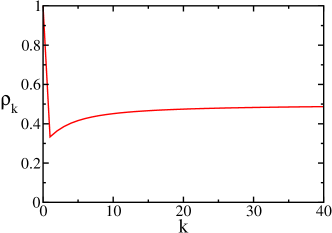
Figure 2: The density profile $\rho_{k}$, obtained from the quasi-static approximation.

Our final assumption is that in the reference frame moving with the front, the system is quasi-static. Indeed, by definition $d\rho_{0}/dt=0$, and we further assume $d\rho_{k}/dt=0$ for all $k$. The stationary density profile is

$$\rho_{k}=\frac{\sum_{j=0}^{k-1}\rho_{j}}{2\sum_{j=0}^{k-1}\rho_{j}+1}.$$ (4)

This recursive equation is solved subject to the boundary condition $\rho_{0}=1$. For small $k$ we have

$$\rho_{k}=1,\frac{1}{3},\frac{4}{11},\frac{56}{145},\qquad k=0,1,2,3,\cdots.$$ (5)

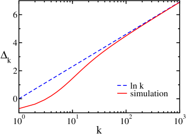
Figure 3: The total excess of empty sites $\Delta_{k}$ versus distance $k$. The simulations are in a system of size $L=1000$.

Despite the crude simplifying assumptions, this quasi-static approximation provides the following valuable insights (see figure 2):

1. Depletion. With the exception of the occupied front, all sites are more likely to be vacant, $\rho_{k}<1/2$ for all $k>0$. In other words, the propagating front includes a depletion zone. This depletion is a direct consequence of the fact that occupied sites change at a higher rate than vacant sites. In other words, vacant sites have a larger lifetime.

2. Monotonicity. The density profile is monotonic, $\rho_{i}>\rho_{j}$ for $i>j\geq 1$.

The tail of the density profile can be obtained by noting that $\rho_{k}\to 1/2$ as follows from (4). Consequently, the average total “mass” to the left of a given site, $m_{k}=\sum_{j=0}^{k-1}\rho_{j}$, grows linearly with distance, $m_{k}\simeq k/2$. At large distances, the recursion equation for the density $\rho_{k}=m_{k}/(2m_{k}+1)$ can be re-written as $\rho_{k}\simeq\frac{1}{2}-\frac{1}{4m_{k}}$ and therefore,

$$\rho_{k}\simeq\frac{1}{2}-\frac{1}{2k}.$$ (6)

Far away from the front, sites are occupied at random as $\rho_{k}\to 1/2$ for $k\to\infty$. Indeed, sites at the tail change their state extremely rapidly at rates that grow linearly with distance. These rapid changes effectively destroy spatial correlations. Moreover, the advancement of the front becomes irrelevant at large distances. Hence, the two assumptions underlying our theory are inconsequential in the tail region and (6) is in fact exact. We comment that the algebraic tail (6) is unusual because traveling waves are typically characterized by exponential tails wvs ; bd .

The cumulative expected excess of vacant sites over occupied sites, $\Delta_{k}=\sum_{j=0}^{k-1}(1-2\rho_{j})$, measures the extent of the depletion zone. This quantity follows from the tail behavior (6), $\Delta_{k}=k-2m_{k}$, and since $m_{k}\simeq(k-\ln k)/2$, the excess of vacant sites grows logarithmically with distance,

$$\Delta_{k}\simeq\ln k.$$ (7)

Thus, the total excess of vacant sites is divergent!

We confirmed the theoretical predictions for the algebraic tail (6) and the logarithmic growth of the excess (7) using massive Monte Carlo simulations (figure 2). The numerical simulations are straightforward. In each simulation step one site is chosen at random. If this site is occupied, the state of the site and all sites to the right change according to (1), but otherwise, nothing happens. After each step, time is augmented by the inverse of the system size $t\to t+L^{-1}$ where $L$ is the number of sites in the lattice. In our implementation, the front is always located at the zeroth site, $\sigma_{0}=1$. Whenever the front advances by $n$ sites, all lattice sites are appropriately shifted to the left, $\sigma_{i}\to\sigma_{i-n}$ (the $n$ rightmost sites are reoccupied at random). Subsequently, the front position is augmented by $n$. This efficient implementation allows us to simulate the evolution of the system up to extremely large times. We can evolve a system of size $L=10^{2}$ up to time $t=10^{11}$, and we obtain statistical averages from snapshots of the system taken at unit time intervals.

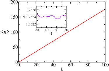
Figure 4: The average position of the leftmost bit $\langle x\rangle$ versus time $t$. The results are from a Monte Carlo simulation in a system of size $L=10^{2}$, evolved up to time $t=10^{11}$. The inset shows the velocity $v=d\langle x\rangle/dt$ versus time.

II.2 Front Propagation

Whenever the leftmost site flips, the front position $x$ advances by $n$ lattice sites,

$$\cdots 0000\underbrace{11111}_{n}0100\cdots\to\cdots 0000\underbrace{00000}_{n}1011\cdots.$$ (8)

Hence, the leftmost string of occupied sites governs the front propagation. Like all other sites, the front flips at a unit rate, and consequently, the average front position grows ballistically,

$$\langle x\rangle\simeq v\,t,$$ (9)

and the propagation velocity $v$ equals the average size of the leftmost occupied string $v=\langle n\rangle$.

Let $S_{n}$ be the probability that the leftmost $n$ lattice sites including the front are all occupied,

$$S_{n}\equiv{\rm Prob}(\underbrace{11111}_{n}).$$ (10)

The probability of finding a string of exact length $n$ as in (8) is equal $S_{n}-S_{n+1}$, and therefore the velocity is given by $v=\langle n\rangle=\sum_{n=1}^{\infty}n(S_{n}-S_{n+1})$. Consequently, the velocity equals the sum of string probabilities

$$v=\sum_{n=1}^{\infty}S_{n}.$$ (11)

In the Quasi-Static Approximation (QSA), correlations between different sites are neglected, and hence, the string probability (10) is a product over the corresponding densities,

$$S^{\rm uncorr}_{n}=\rho_{1}\rho_{2}\cdots\rho_{n-1},$$ (12)

for $n>1$ while $S_{1}=1$. With this approximate expression, the propagation velocity is $v=1+\rho_{1}+\rho_{1}\rho_{2}+\rho_{1}\rho_{2}\rho_{3}+\cdots$. We obtain the approximate velocity

$$v_{\rm QSA}=1.534070$$ (13)

by substituting the densities from (4) into (12) and then summing numerically. The velocity (13) obeys the obvious bounds $1\leq v\leq 2$. The lower bound reflects that the front must advance by at least one lattice site, and the upper bound corresponds to the completely random configuration, $\rho_{k}=1/2$ and $S_{n}=2^{-(n-1)}$.

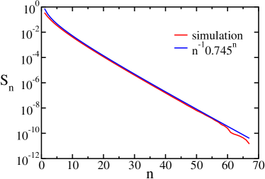
Figure 5: The string probability $S_{n}$ versus the string length $n$. The results are from a Monte Carlo simulation in a system of size $L=200$, evolved up to time $t=10^{11}$.

The numerical simulations confirm that the front advances ballistically (figure 4) but the propagation velocity is larger than the value predicted by the quasi-static approximation

$$v_{\rm MC}=1.7624\pm 0.0001.$$ (14)

Strong spatial correlations are primarily responsible for the discrepancy between (13) and (14). Indeed, if we substitute the densities $\rho_{k}$ obtained from the Monte Carlo simulations into the product expression (12) and perform the summation in (11), we obtain the value $v=1.5329\pm 0.0001$ that is surprisingly close to the quasi-static approximation (13). We therefore conclude that spatial correlations between neighboring sites have a significant effect on the velocity.

II.3 Correlations, Aging, and Rejuvenation

Spatial structures and spatial correlations can be quantified in multiple ways and we focus on the likelihood of occupied strings $S_{n}$. Numerically, we find that this quantity decays exponentially (figure 5),

$$S_{n}\sim n^{-\nu}\lambda^{n},$$ (15)

as $n\to\infty$ with $\lambda=0.745\pm 0.001$ and $\nu\approx 1$. The quasi-static approximation yields much more rapid decay, $\lambda=1/2$ and $\nu=1$ as follows from the algebraic tail (6) and the product expression (12). Of course, when sites are completely uncorrelated, one also has $\lambda=1/2$. The fact that $\lambda$ is larger than $1/2$ reflects that the system is strongly correlated. There is a significant enhancement of strings of consecutively occupied sites and this enhancement is largely responsible for the larger velocity (14).

Even though spatial correlations are significant and affect quantities of interest such as the velocity, they are limited in extent as indicated by the exponential decay of the string likelihood. For this reason, numerical simulations may be performed in relatively small systems. Given the spatial extent of strings shown in figure 5, we performed the simulations using a relatively small system, $L=200$. This system size is used throughout this investigation, unless noted otherwise.

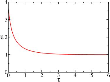
Figure 6: The velocity $u$ versus age $\tau$.

We also probed the correlation between two successive front “jumps” as a measure of temporal correlations. Let $n$ and $n^{\prime}$ be the sizes of two consecutive jumps, respectively. If the front advances via a renewal process then $\langle nn^{\prime}\rangle=\langle n\rangle^{2}=v^{2}$. However, the numerical simulations yield $\langle n\,n^{\prime}\rangle=2.959\pm 0.001$ while $v^{2}=3.1060\pm 0.0001$. Thus, front advancement events are correlated, so the state of the system just after a jump is correlated with the state of the system just before a jump.

This temporal correlation affects, in particular, the diffusion coefficient $D$ that quantifies the uncertainty in the front position,

$$\langle x^{2}\rangle-\langle x\rangle^{2}\simeq 2Dt.$$ (16)

Numerically, we find $D=2.856\pm 0.001$. In contrast with the velocity (11) that follows from average quantities such as the average segment density, the diffusion coefficient requires more detailed information about temporal correlations note .

To further characterize the dynamics, we define the age $\tau$ as the time elapsed since the most recent front jump. Moreover, we define the age-dependent velocity $u(\tau)$ as the average size of the leftmost string $n$ as in (8) at age $\tau$ because this quantity governs the front propagation. The simulations show that the velocity rapidly decays with age (figure 6). Of course, since long-living fronts outlive any of their occupied neighbors, $u\to 1$ as $\tau\to\infty$. Aging fronts are therefore sluggish. In contrast, newly-born fronts are much more vigorous because $u(0)>v$. Since the flipping process is completely random, the survival probability of a configuration decays exponentially with age. The average velocity in (11) is the weighted integral of the age-dependent velocity

$$v=\int_{0}^{\infty}d\tau\,u(\tau)\,e^{-\tau},$$ (17)

and the weight equals the exponential survival probability.

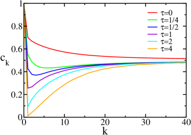
Figure 7: The density profile $c_{k}$ versus distance $k$ at different ages.

The age-dependence of the velocity implies that the shape of the front must also be age-dependent. We therefore measured the density profile $c_{k}(\tau)=\langle\sigma_{k}(\tau)\rangle$, defined as the average occupation at distance $k$ from the front at age $\tau$. We find interesting evolution with age. The profile of long-living fronts has a depletion zone and is qualitatively similar to the average profile discussed above, but the profile of newly born fronts has an enhancement of occupied sites over vacant sites (figure 7). This rejuvenation is intuitive: the state of the system just after a jump is a mirror image of the state of the system just before the jump. Long living fronts are followed by a large string of vacant sites, and these fronts are necessarily slow. Yet, upon flipping, such sluggish fronts rejuvenate as the string of vacant sites become a string of occupied sites. Interestingly, the density profile may even be non-monotonic at intermediate ages.

In conclusion, the flipping process involves all the hallmarks of nonequilibrium dynamics including spatial correlations, temporal correlations, aging, and rejuvenation vp .

II.4 Small Segments

We complete the analysis with a direct solution for the state of small segments containing the front. The $k$ leftmost sites can be in any one of $2^{k-1}$ possible configurations. The equations describing the configuration probabilities are hierarchical: due to the front motion, the state of small segments containing the front is coupled with the state of larger segments. To overcome this closure issue, we propose an approximation where the state of the system outside the segment of interest is completely random, as in our simulation method. Clearly, this approximation becomes exact as $k\to\infty$.

A segment of length two can be in one of two configurations: $10$ or $11$. The respective probabilities $P_{10}$ and $P_{11}$ evolve according to

$$\frac{dP_{10}}{dt} =-P_{10}+P_{11}+\frac{1}{2}\,P_{11}+\frac{1}{2}\,P_{10}$$ (18a)

$$\frac{dP_{11}}{dt} =-2P_{11}+\frac{1}{2}\,P_{11}+\frac{1}{2}\,P_{10}\,.$$ (18b)

We explain the latter equation in detail. The loss rate in (18b) equals two because any of the two occupied sites may flip. If the front flips, there is advancement, and since the second site is occupied with probability $1/2$, the gain terms are $\frac{1}{2}P_{11}$ and $\frac{1}{2}\,P_{10}$. The steady state solution is $(P_{10},P_{11})=\frac{1}{4}(1,3)$; therefore $\rho_{1}=1/4$. We denote by $v_{k}$ the velocity obtained from a segment of length $k$. For $k=2$ we have $v_{2}=P_{10}+3P_{11}$ since the front advances by one site when the front flips in the state $10$, but it advances three sites in the state $11$ (two sites plus an average of one, given the random occupation outside the segment).

$k$	$v_{k}^{(0)}$	$v_{k}^{(1)}$	$v_{k}^{(2)}$	$v_{k}^{(3)}$	$v_{k}^{(4)}$
2	1.500000
3	1.535714	1.418947
4	1.587165	1.826205	1.779225
5	1.629503	1.773099	1.765862	1.764458
6	1.662201	1.766730	1.764592	1.758245	1.762322
7	1.687108	1.765129	1.763533	1.770104	1.765175
8	1.705987	1.764330	1.762272	1.761669
9	1.720251	1.763754	1.761864
10	1.730993	1.763313
11	1.739055

Table 1: The velocity $v$, obtained by successive iterations of the Shanks transformation (propagating fronts).

For $k=3$, the governing equations are

$$\frac{dP_{100}}{dt} =-P_{100}+\frac{3}{2}P_{101}+\frac{1}{4}P_{110}+\frac{5}{4}P_{111}$$ (19a)

$$\frac{dP_{101}}{dt} =-\frac{3}{2}P_{101}+\frac{5}{4}P_{110}+\frac{1}{4}P_{111}$$ (19b)

$$\frac{dP_{110}}{dt} =\frac{1}{2}P_{100}-\frac{7}{4}P_{110}+\frac{5}{4}P_{111}$$ (19c)

$$\frac{dP_{111}}{dt} =\frac{1}{2}P_{100}+\frac{1}{4}P_{110}-\frac{11}{4}P_{111}.$$ (19d)

The steady state solution is $(P_{100},P_{101},P_{110},P_{111})=\frac{1}{56}(27,11,12,6)$; thus, the densities are $\rho_{1}=9/28$, and $\rho_{2}=17/56$ and the velocity is $v_{3}=43/28$. Furthermore, $v_{4}=10907/6872$ and the approximation steadily improves as $k$ increases.

We can compute the configuration of segments with $k\leq 12$ as detailed in Appendix A. To extrapolate the velocity, we use the Shanks transformation bo

$$v_{k}^{(m+1)}=\frac{v_{k-1}^{(m)}v_{k+1}^{(m)}-v^{(m)}_{k}v^{(m)}_{k}}{v^{(m)}_{k-1}+v^{(m)}_{k+1}-2v^{(m)}_{k}}$$ (20)

where $v_{n}^{(m)}$ is the velocity estimate after $m$ iterations. Repeated Shanks transformations give a useful estimate for the propagation velocity (see Table II),

$$v_{\rm shanks}=1.76\pm 0.01.$$ (21)

The Shanks transformation can be used to estimate other quantities as well. For example, we obtain an excellent estimate for the density of the first site, $\rho_{1}=0.3492\pm 0.0001$.

III Pinned Fronts

As discussed above, the quasi-static approximation neglects the movement of the front and possible correlations between sites. Of these two assumptions, the latter is more significant. We therefore modify the original flipping process and forbid the front from changing state. This minor modification pins the front and allows us to focus on the role of correlations.

In the pinned process, a flip event at every site other than the origin changes the state of the system exactly as in (1), but a flip event at the origin yields

$$\sigma_{i}\to 1-\sigma_{i},\quad{\rm for\ all}\quad i>0.$$ (22)

Hence, the site at the origin is always occupied, $\sigma_{0}(t)=1$.

Remarkably, pinning the front results in only minor quantitative changes. All quantities of interest including the velocity $v$, the diffusion coefficient $D$, the decay constant underlying the decay of the segment density $\lambda$, and the density profile $\rho_{k}$ are all within a few percent of the corresponding values for propagating fronts (Table II). In particular, the discrepancy in the propagation velocity is smaller than $1\%$,

$$v_{\rm pinned}=1.7753\pm 0.0001.$$ (23)

We note that the velocity and the diffusion coefficient are obtained by using the running total of segment lengths at the time when the origin causes a flip as a surrogate for the front position $x$. Finally, we can not exclude the possibility that the string probability $S_{n}$ is characterized by the same parameter $\lambda$ in both processes (Table II).

quantity	propagating fronts	pinned fronts
$v$	$1.7624$	$1.7753$
$D$	$2.856$	$3.178$
$\lambda$	$0.74$	$0.75$
$\rho_{1}$	$0.3492$	$1/3$
$\rho_{2}$	$0.3400$	$1/3$
$\rho_{3}$	$0.3479$	$41/120$

Table 2: The velocity $v$, the diffusion coefficient $D$, the decay constant governing the string probability $\lambda$, and the first few densities $\rho_{k}$ for propagating and pinned fronts. The results are from Monte Carlo simulations in a system of size $L=200$ evolved up to time $t=10^{11}$. The exact solution for the density profile is detailed below.

In addition, pinned fronts and propagating fronts have very similar density profiles (figure 8). The quasi-static approximation, which is better suited for pinned fronts, becomes slightly more accurate. Of course, the exact tail behavior (6) and the logarithmic excess (7) extend to pinned fronts.

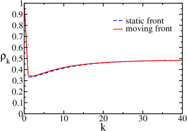
Figure 8: The density $\rho_{k}$ versus distance $k$ for pinned and propagating fronts. Both profiles are obtained using Monte Carlo simulations.

III.1 Correlations

The hierarchical evolution equation (3) for the average occupation only assumes that the front is pinned and hence, this equation provides an exact description. Therefore, the single-site averages and the two-site averages are related,

$$\langle\sigma_{k}\rangle-\sum_{j=0}^{k-1}\langle\sigma_{j}\rangle=-2\sum_{j=0}^{k-1}\langle\sigma_{j}\sigma_{k}\rangle,$$ (24)

at the steady state. Of course, $\langle\sigma_{0}\rangle=1$.

We can obtain the nearest-neighbor correlation $\langle\sigma_{k}\sigma_{k+1}\rangle$, a quantity that evolves according to

$$\frac{d\langle\sigma_{k}\sigma_{k+1}\rangle}{dt}= - \left\langle\left(2+\sum_{j=0}^{k-1}\sigma_{j}\right)\sigma_{k}\sigma_{k+1}\right\rangle$$ (25)

$$+\langle(1-\sigma_{k})\sigma_{k+1}\rangle + \left\langle\left(\sum_{j=0}^{k-1}\sigma_{j}\right)(1-\sigma_{k})(1-\sigma_{k+1})\right\rangle.$$

This equation is very similar to the equation governing the one-site correlation. The rate of change for two occupied sites is $2+\sum_{j=0}^{k-1}\sigma_{j}$ because either one of the two sites can flip. In general, the equation for two-site correlations involves three-site correlations, but in the particular case of neighboring sites, the three-site correlation cancels in (25)! We therefore obtain a relation between average densities and two-site correlations

$$\sum_{j=0}^{k-2}\langle\sigma_{j}\rangle=\langle\sigma_{k-1}\sigma_{k}\rangle+\sum_{j=0}^{k-2}\langle\sigma_{j}\sigma_{k-1}\rangle+\sum_{j=0}^{k-1}\langle\sigma_{j}\sigma_{k}\rangle.$$ (26)

There are two different relations between the average density and the two-site correlation: equations (24) and (26). By manipulating the two, we obtain the nearest-neighbor correlation in terms of the average density,

$$\langle\sigma_{k}\sigma_{k+1}\rangle=\frac{1}{2}\,\langle\sigma_{k+1}\rangle$$ (27)

for $k>0$. This relation demonstrates that neighboring sites are positively correlated,

$$\langle\sigma_{k}\sigma_{k+1}\rangle-\langle\sigma_{k}\rangle\langle\sigma_{k+1}\rangle=\bigg{(}\frac{1}{2}-\langle\sigma_{k}\rangle\bigg{)}\,\langle\sigma_{k+1}\rangle.$$ (28)

We also note that correlations decay slowly at large distances as equations (6) and (28) imply $\langle\sigma_{k}\sigma_{k+1}\rangle-\langle\sigma_{k}\rangle\langle\sigma_{k+1}\rangle\simeq(4k)^{-1}$.

For completeness, we mention that the correlation between three consecutive sites can also be written as a function of lower-order correlations

$$\langle\sigma_{k}\sigma_{k+1}\sigma_{k+2}\rangle=\frac{1}{2}\langle\sigma_{k+2}(1-\sigma_{k})\rangle.$$ (29)

III.2 Small Systems

When the front is pinned, the system reaches a stationary state. This steady state can be obtained exactly for small system by considering the evolution of all possible configurations. For pinned fronts, finite segments are not affected by flipping outside the segment, and consequently, the evolution equations are now closed.

Consider for example a system with two sites. There are two possible configurations: $10$ and $11$ with the respective probabilities $P_{11}$ and $P_{10}$. These probabilities evolve according to

$$\frac{dP_{10}}{dt} =-P_{10}+2P_{11}$$ (30a)

$$\frac{dP_{11}}{dt} =-2P_{11}+P_{10}.$$ (30b)

Hence, at the steady state, $(P_{10},P_{11})=\frac{1}{3}(2,1)$ and consequently, $\rho_{1}=S_{2}=1/3$.

$k$	$\rho_{k}$	$S_{k+1}$	$v_{k+1}$
0	$1$	$1$	$1$
1	$\frac{1}{3}$	$\frac{1}{3}$	$\frac{4}{3}$
2	$\frac{1}{3}$	$\frac{1}{6}$	$\frac{3}{2}$
3	$\frac{41}{120}$	$\frac{23}{240}$	$\frac{383}{240}$
4	$\frac{76121}{216000}$	$\frac{25577}{432000}$	$\frac{714977}{432000}$

Table 3: The density $\rho_{k}$, the string density $S_{k}$, and the velocity $v_{k}=\sum_{n=1}^{k}P_{n}$, obtained by direct solution of the microscopic evolution equations.

Next we consider the first three sites with the four configurations $100$, $101$, $110$, $111$. The evolution equations for the respective probabilities are

$$\frac{dP_{100}}{dt} =-P_{100}+P_{110}+P_{111}+P_{101}$$ (31a)

$$\frac{dP_{101}}{dt} =-2P_{101}+2P_{110}$$ (31b)

$$\frac{dP_{110}}{dt} =-2P_{110}+P_{101}+P_{111}$$ (31c)

$$\frac{dP_{111}}{dt} =-3P_{111}+P_{100}.$$ (31d)

The steady state solution is $(P_{100},P_{101},P_{110},P_{111})=\frac{1}{6}(3,1,1,1)$. Therefore $\rho_{1}=\rho_{2}=1/3$ and $S_{3}=1/6$. Results for $k\leq 4$ are summarized in table 3.

$k$	$v_{k}^{(0)}$	$v_{k}^{(1)}$	$v_{k}^{(2)}$	$v_{k}^{(3)}$	$v_{k}^{(4)}$
1	1.
2	1.333333	1.666666
3	1.5	1.72549	1.769737
4	1.595833	1.750742	1.773156	1.775020
5	1.655039	1.762616	1.774362	1.775178	1.775278
6	1.693228	1.768521	1.774849	1.775239	1.775289
7	1.718565	1.771576	1.775065	1.775267	1.775293
8	1.735709	1.773205	1.775170	1.775280	1.775293
9	1.747473	1.774095	1.775223	1.775287
10	1.755632	1.774593	1.775252
11	1.761337	1.774876
12	1.765350

Table 4: Iterated Shanks transformations for the velocity. The zeroth column is from the small system solution (pinned fronts).

In general, there are $2^{k-1}$ microscopic configurations in a system of size $k$. We can compute the stationary probabilities for systems of size $k\leq 12$ as detailed in Appendix B. Knowledge of these steady state probabilities yields the density $\rho_{k}$, the string probability $S_{k}$, and hence, an estimate for the velocity $v_{k}=\sum_{n=1}^{k}S_{n}$.

The velocity, as well as other quantities of interest, can be obtained very accurately using the Shanks transformation. We find $v_{\rm shanks}=1.7753\pm 0.0001$, in perfect agreement with the Monte Carlo simulations (23) as shown in Table 4.

III.3 Aging and Rejuvenation

We also examined the evolution with age and found that pinned and propagating fronts display very similar behaviors, as evident from the age-dependent density $c_{k}(\tau)$ (figure 9).

For pinned fronts, the zero age configuration is the exact mirror image of the configuration just before the flip and since the front flips at random,

$$c_{k}(\tau=0)=1-\rho_{k}$$ (32)

for all sites except the origin, $k>0$. This expression demonstrates the enhancement of occupied sites for newly born configurations.

Aging can be conveniently studied using small systems. For the first site, we have $dc_{1}/d\tau=-c_{1}$ and therefore, $c_{1}(\tau)=c_{1}(0)e^{-\tau}$. The initial condition, $c_{1}(0)=1-\rho_{1}=2/3$ follows from (32). Therefore,

$$c_{1}(\tau)=\frac{2}{3}e^{-\tau}.$$ (33)

For the first two sites, there are four configurations: $100$, $101$, $110$, $111$, and the respective probabilities evolve according to

$$\frac{dP_{100}}{d\tau} =P_{111}+P_{101}$$ (34a)

$$\frac{dP_{101}}{d\tau} =-P_{101}+P_{110}$$ (34b)

$$\frac{dP_{110}}{d\tau} =-P_{110}+P_{111}$$ (34c)

$$\frac{dP_{111}}{d\tau} =-2P_{111}.$$ (34d)

These equations differ from (31) in that flipping events caused by the front are excluded. The initial condition again mirrors the stationary state $(P_{100},P_{101},P_{110},P_{111})\big{|}_{\tau=0}=\frac{1}{6}(1,1,1,3)$. By solving the evolution equations, the age-dependent density of the second site, $c_{2}=P_{101}+P_{111}$, is

$$c_{2}(\tau)=\frac{1}{3}(2\tau-1)e^{-\tau}+e^{-2\tau}.$$ (35)

Already, we can justify the non-monotonic behavior seen in figures (7) and (9): $c_{1}>c_{2}$ for $\tau<\tau_{*}$ with $\tau_{*}=0.8742$ while $c_{1}<c_{2}$ for otherwise. In general, all densities exhibit a simple exponential decay with age, $c_{k}(\tau)\propto e^{-\tau}$ as $\tau\to\infty$. We conclude that pinned fronts faithfully capture aging and rejuvenation.

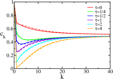
Figure 9: The density $c_{k}$ at different ages for pinned fronts (broken lines) and propagating fronts (solid lines).

IV Conclusions

In conclusion, we reformulated the bit flipping process underlying the simplex algorithm as a nonequilibrium dynamics problem and studied spatial and temporal properties using theoretical and computational methods. Overall, we find that the infinite interaction range leads to rich phenomenology. There is a front that propagates ballistically with a nontrivial velocity that is governed by the length of the occupied strings containing the front. The propagating front includes a deep depletion zone: vacant sites outnumber occupied sites with the total excess of unoccupied sites growing logarithmically with depth. The flipping process is characterized by significant spatial correlations. For example, the likelihood of finding strings of consecutively occupied sites is strongly enhanced.

The flipping process also exhibits nontrivial dynamics. Successive front jumps are correlated and additionally, there are aging and rejuvenation as young fronts are fast but old fronts are slow. Underlying this behavior is the fact that the state of the system just after a jump mirrors the state of the system just before a jump.

We slightly modified the original flipping process by pinning the front. Qualitatively and quantitatively, pinned fronts and propagating fronts are very close. We demonstrated analytically much of the interesting phenomenology including spatial correlations, aging, and rejuvenation for pinned fronts.

Aging is usually characterized by using two different times ckp . Here, in contrast, the time elapsed since the latest front yields a natural definition of age and a characterization of the dynamics that complements time itself.

We comment that there is an alternative way of studying the density profile through an average at a given lattice site over all realizations rbd . The corresponding average density $\tilde{\rho}_{k}(t)$ reaches a stationary form once the average and the variance are taken into account,

$$\tilde{\rho}_{k}(t)\to\Phi\left(\frac{k-vt}{\sqrt{Dt}}\right)$$ (36)

with $\Phi(-\infty)=0$ and $\Phi(\infty)=1/2$. This approach has a disadvantage: the scaling function $\Phi(x)$ is dominated by fluctuations in the position of the front. In other words, the density profile $\rho_{k}$ is smeared because of diffusion. These less interesting diffusive fluctuations are suppressed when the front profile is probed in a reference frame moving with the front.

We also presented a systematic solution method of small systems and successfully demonstrated how to extrapolate relevant parameters for infinite systems. Yet, since the complexity grows exponentially with system size, such computations quickly become prohibitive. We have also seen how most quantities of interest require an infinite hierarchy of equations. Finding an appropriate theoretical framework with closed evolution equations remains a formidable challenge. Nevertheless, the pinned front process provides a powerful theoretical framework.

Appendix A Transition matrix for propagating fronts

The evolution equations for the configuration probabilities in a finite segment of size $k$ can be represented in the matrix form

$$\frac{d{\bf P}}{dt}=\mathcal{M}{\bf P}.$$ (37)

Here, ${\bf P}$ is the vector ${\bf P}=\{P_{1j}\,|0\leq j\leq U-1$} where $j$, written as a binary, is in increasing order and $U=2^{k-1}$. For example, when $k=5$ the state vector is $(P_{10000},P_{10001},\cdots,P_{11111})$, with $U=16$ entries. The elements of this vector equal the probabilities that the system is in the respective configuration. Also, $\mathcal{M}$ is the $U\times U$ transition matrix whose elements equal the transition rates between the corresponding configurations.

The transition matrix $\mathcal{M}$ is a sum of three matrices

$$\mathcal{M}=\mathcal{M}_{1}+\mathcal{M}_{2}+\mathcal{M}_{3}.$$ (38)

We quote the first two for $k=5$,

$$\mathcal{M}_{1}=\left(\begin{array}[]{rrrrrrrrrrrrrrrr}0&1&&1&&&&1&&&&&&&&1\\ &&1&&&&1&&&&&&&&1&\\ &&&1&&1&&&&&&&&1&&\\ &&&&1&&&&&&&&1&&&\\ &&&&&1&&1&&&&1&&&&\\ &&&&&&1&&&&1&&&&&\\ &&&&&&&1&&1&&&&&&\\ &&&&&&&&1&&&&&&&\\ &&&&&&&&&1&&1&&&&1\\ &&&&&&&&&&1&&&&1&\\ &&&&&&&&&&&1&&1&&\\ &&&&&&&&&&&&1&&&\\ &&&&&&&&&&&&&1&&1\\ &&&&&&&&&&&&&&1&\\ &&&&&&&&&&&&&&&1\\ &&&&&&&&&&&&&&&0\end{array}\right)$$

and

$$\mathcal{M}_{2}=\frac{1}{16}\times\left(\begin{array}[]{rrrrrrrrrrrrrrrr}&&&&&&&8&&&&4&&2&1&1\\ &&&&&&&8&&&&4&&2&1&1\\ &&&&&&8&&&&&4&&2&1&1\\ &&&&&&8&&&&&4&&2&1&1\\ &&&&&8&&&&&4&&&2&1&1\\ &&&&&8&&&&&4&&&2&1&1\\ &&&&8&&&&&&4&&&2&1&1\\ &&&&8&&&&&&4&&&2&1&1\\ &&&8&&&&&&4&&&2&&1&1\\ &&&8&&&&&&4&&&2&&1&1\\ &&8&&&&&&&4&&&2&&1&1\\ &&8&&&&&&&4&&&2&&1&1\\ &8&&&&&&&4&&&&2&&1&1\\ &8&&&&&&&4&&&&2&&1&1\\ 8&&&&&&&&4&&&&2&&1&1\\ 8&&&&&&&&4&&&&2&&1&1\end{array}\right)$$

The third matrix $\mathcal{M}_{3}$ is diagonal and it guarantees that each column of $\mathcal{M}$ sums to zero. We note that the transition matrix is sparse. The steady state probability equals the zeroth eigenvector, $\mathcal{M}{\bf P}=0$. Finally, the velocity follows from the average advancement expected in each configuration. This advancement is represented by the vector ${\bf J}$ and for example, ${\bf J}=(1,1,1,1,1,1,1,1,2,2,2,2,3,3,4,6)$ for $k=5$. The velocity is simply the scalar product, $v={\bf J}\cdot{\bf P}$.

Appendix B Transition matrix for pinned fronts

Using the matrix notation in (37), the evolution equations for $k=4$ involve the following transition matrix

$$\mathcal{M}=\left(\begin{array}[]{rrrrrrrr}-1&1&&1&&&&2\\ \\ &-2&1&&&&2&\\ \\ &&-2&1&&2&&\\ \\ &&&-3&2&&&\\ \\ &&&1&-2&1&&1\\ \\ &&1&&&-3&1&\\ \\ &1&&&&&-3&1\\ \\ 1&&&&&&&-4\\ \end{array}\right).$$ (39)

In this case, the steady state probabilities are

$${\bf P}=\left(\begin{array}[]{c}P_{1000}\\ P_{1001}\\ P_{1010}\\ P_{1011}\\ P_{1100}\\ P_{1101}\\ P_{1110}\\ P_{1111}\end{array}\right)=\frac{1}{240}\times\left(\begin{array}[]{c}92\\ 28\\ 22\\ 18\\ 27\\ 13\\ 17\\ 23\end{array}\right)$$ (40)

Thus, the density is $\rho_{3}=41/120$ and the string probability is $P_{4}=23/240$.