PTA–07–054

Bottom-Up Reconstruction Scenarios for
(un)constrained MSSM Parameters at the LHC
J.-L. Kneur¹ and N. Sahoury<sup>1,2

1</sup> Laboratoire de Physique Théorique et Astroparticules, UMR5207–CNRS,

Univ. Montpellier 2, FR-34095 Montpellier Cedex 5, France.

² Laboratoire de Physique Nucl aire et Hautes Energies, UMR7585–CNRS, Univ. Paris VI, FR-75252 Paris Cedex 5, France.

Abstract:

We consider some specific inverse problem or “bottom-up” reconstruction strategies at the LHC for both general and constrained MSSM parameters, starting from a plausibly limited set of sparticle identification and mass measurements, using mainly gluino/squark cascade decays, plus eventually the lightest Higgs boson mass. For the three naturally separated sectors of: gaugino/Higgsino, squark/slepton, and Higgs parameters, we examine different step-by-step algorithms based on rather simple, entirely analytical, inverted relations between masses and basic MSSM parameters. This includes also reasonably good approximations of some of the relevant radiative correction calculations. We distinguish the constraints obtained for a general MSSM from those obtained with universality assumptions in the three different sectors. Our results are compared at different stages with the determination from more standard “top-down” fit of models to data, and finally combined into a global determination of all the relevant parameters. Our approach gives complementary information to more conventional analysis, and is not restricted to the specific LHC measurement specificities. In addition, the bottom-up renormalization group evolution of general MSSM parameters, being an important ingredient in this framework, is illustrated as a new publicly available option of the MSSM spectrum calculation code “SuSpect”.

I Introduction

If supersymmetry shows up at the LHC, it may be that only a limited part of the predicted Minimal Supersymmetric Standard Model (MSSM)MSSM sparticles will be discovered and some of their properties measured. Hopefully, the lightest Higgs scalar $h$ could be discovered, and some of the squarks and the gluino could be copiously produced (if not too heavy) at the LHC due to their strong interactions. In addition some of the neutralinos, including the lightest supersymmetric sparticle (LSP), could be identified and have their masses extracted indirectly from a detailed study of squark and gluino cascade decayscascade ; cascade1 ; cascade2 . Beyond that, the discovery and measurement of the full set of MSSM sparticles may be very model dependent, and anyway challenging in many scenarios at the LHC. Various analyses have been conducted (see e.g. LHCstudy ; SPA ) to determine the basic MSSM parameter space from the above assumed experimental measurements. A widely illustrated strategy, in a so-called “top-down” approach, is to start from a given supersymmetry-breaking model at a very high grand unification scale; predict for given input parameter values the superpartner spectrum at experimentally accessible energy scales; then fit this spectrum (together with possibly other observables like cross-sections etc) to the data in order to extract constraints on the basic model parameters. Constraints from past and present collider and non-collider data, with consequent prospects for the LHC and future linear collider (ILC), have been analyzed typically from systematic scanning of MSSM parameter spacemsugrascan ; mssmbayes (though mostly in the constrained minimal supergravity (mSUGRA) mSUGRA case). In addition, more elaborated $\chi^{2}$ fitting procedure (or some generalizationspdg ; minuit ) have been also used in many such studies, together with Monte-Carlo or other process simulation toolsPythia ; Herwig ; Comphep , as well as other specific codes for parameter determinationSfitter ; Fittino . On general grounds, fitting and minimization procedures are efficient when the number of independent measurements is (much) greater than the number of fitted parameters of the underlying model, and provided that data are reasonably accurate. But clearly the minimization becomes less controllable in a general MSSM with more than $\sim$ 20 relevant basic parameters (even when neglecting flavor mixing in the sfermion sector). Alternatively, so-called inverse or bottom-up reconstruction approaches are often motivatedinv1 ; zerwasetal ; bpzm123 ; bpzm_next ; SPA ; kane ; otherinv . Also, a growing number of analysis for the LHC or the ILC appeared recently, attempting to go beyond conventional top-down fitting techniquesotherinv or supplementing these with more elaborated frequentist or Bayesian methods, with Markov chain Monte-Carlo (MCMC) techniquesmarkov in particularmssmbayes ; ben_bayes ; dzerwas . Yet it has been stressed (for instance in refs. otherinv ) that the mapping from LHC data to the underlying basic MSSM parameters may be far from unique. However, most works still rely essentially on simulation tools fed with top-down MSSM Lagrangian-to-spectrum relations, while to our knowledge reconstruction scenarios based on explicitly inverted relations (see e.g. inv1 ; zerwasetal ; bpzm123 ; bpzm_next ) appear not so widely explored in the literature. Moreover, many studies on MSSM parameter reconstructionFittino ; LHCstudy ; SPA often considered rather optimistic LHC or ILC scenarios, in the sense that the results presented were obtained by assuming that most, if not all, MSSM sparticles masses and other relevant observables are measured with the best expected accuracy. At the same time it is often assumed that the more constrained mSUGRA modelmSUGRA (with four continuous plus one discrete parameters) is to be determined. While such studies are certainly very useful guidelines for LHC and ILC analysis, these assumptions may be considered quite optimistic for the supersymmetry discovery prospects in general, especially at the LHC. It is thus worth to develop alternative (or rather complementary) strategies to foresee more pessimistic scenarios, still trying to extract as much as possible informations on the nature of the underlying supersymmetry-breaking model in case where only a handful of the predicted sparticles would be identified.

To start with, in this paper we explore specific bottom-up reconstructions, which are more restricted and certainly far from being fully realistic as concerns data simulations, but that we expect to be useful and complementary to the more standard simulation tools. Our approach is based essentially on analytical inverse relations between the measured masses and basic parameters. This “inverse mapping” for the MSSM spectrum has been investigated to some extent in the past yearsinv1 ; zerwasetal but mainly at the tree-level approximation, and moreover much often in the context of the ILC data essentially. It is generally expected that simple analytic expressions between observables and parameters are more transparent or insightful than purely numerical results, providing e.g. explicit correlations among parameters. Particularly in the MSSM, even at tree-level, this connexion is already quite involved so that it is difficult to grasp with a good intuition the sensitivity of the different observables to MSSM parameters, unless having spend much time in doing fits and related calculations. But more concretely than a useful insight, we also hope that such an approach could suggest new strategies for reconstruction of parameters, as will be illustrated here. For example, by exploiting well-known relations between the (first two generation) squark and slepton soft mass parameters and physical masses, including the renormalization group evolution (RGE) dependencerge ; RGE2 , we construct appropriate combinations of observables in this squark/slepton sector which appear to provide interesting and almost model-independent constraints.
Deriving analytic inversion relations in the MSSM may appear at first a rather academic exercise, quite remote from the complexity of the actual experimental situation especially at the LHC. This is because such inverted mapping remains relatively simple only if restricted to the tree-level approximation. But it becomes a priori inextricable if including radiative corrections, which are certainly necessary at the accuracy level expected for realistic LHC and ILC data analysis. More precisely through loop contributions almost all sparticle masses have a cumbersome dependence on almost all MSSM parameters. Still, we will see how radiative corrections can be incorporated into our framework rather simply, essentially by (numerical) iterative procedure in a manageable way, in reasonable but often realistic approximations. We emphasize that this procedure is very similar to the way in which radiative corrections are included in more conventional top-down MSSM spectrum calculationsisasugra ; suspect ; softsusy ; spheno , and it allows to keep most advantages of the bottom-up approach.

Even if one can incorporate a fair amount of presently know radiative corrections into this framework, we stress that our motivation is not to compete with the state of the art in present analysis of MSSM constraints at LHC, merely by replacing elaborated simulations tools with a bunch of rather simple analytic relations (and simple combinations of data uncertainties as we will see). Accordingly our analysis at this stage is still essentially a theoretical exercise, not incorporating important ingredients of the complexity of LHC measurements (such as detailed event selections, detector properties etc) that are ultimately necessary and that pave the non-trivial steps in going from basic LHC data to sparticle mass measurements. Yet our aim is to consider as much as possible realistic and minimal LHC sparticle identifications, using a limited set of sparticle mass measurements. We then gradually consider different SUSY-discovery scenarios, going from minimal input assumptions to more optimistic ones, defining corresponding algorithms with definite input/output parameters. This step-by-step analysis may turn out to be closer to the actual experimental situation, in which one will certainly not identify all sparticles at once, even for the most optimistic expectations. However our approach is only one step in the vastly more ambitious program of so-called “blind” analysis of LHC data: in particular when we consider a general MSSM case (i.e. departing from e.g. mSUGRA universality relations), we nevertheless assume a spectrum pattern still allowing gluino/squark (long) cascade decays (i.e. with some neutralinos sufficiently heavy to decay in the LSP plus sfermions, but sufficiently light to be decay product of heavier squarks/gluinos). This pattern may admittedly be considered a not so general scenario within the MSSM.
Though our analysis essentially concentrates on sparticles expected to be accessible at the LHC, it will appear that some of the reconstruction algorithms used here could apply more or less directly to ILC measurements, upon appropriate changes in data accuracies. We thus occasionally make some comments on ILC prospects, but refrain to enter a detailed ILC analysis which is beyond the scope of the present paper, since the other expected sparticle mass measurements at the ILC would need rather different algorithms (though quite similar in spirit).

The paper is organized as follows: in section 2 we briefly define and review a plausible set of sparticle mass measurements at the LHC, with accuracy on which is based our analysis. We consider different levels of assumptions on the nature and number of identified sparticles, defining several scenarios. We also gradually introduce universality assumptions for the soft-SUSY breaking parameters of the different sectors. In sections 3–6 we expand results of analytic inversion analysis, with some of these already presented in ref. inv1 , for different parameter sectors of the MSSM, recasting results in the context of gluino/squark cascade decay mass measurements at the LHC, and incorporating radiative corrections. We consider separately four different sectors: gaugino/Higgsino parameters (section 3); squarks and sleptons (first and second generation) (section 4); third generation squarks (section 5); and finally the Higgs parameter sector in section 6. These distinctions are quite natural when considering both the interdependence between observables and parameters and the experimental signatures which are expected at LHC from a given sector. We will delineate which relations and results are valid in a general (unconstrained) or a more constrained MSSM (with universality relations at the GUT scale). We also compare in some detail at different stages our reconstruction results with more standard top-down fitting procedure using MINUIT $\chi^{2}$ minimizationminuit , with data and fitted parameters directly set by the above step-by-step scenarios, rather than by performing “all at once” global fits. Conclusion and outlook are given in section 7.

Finally we develop in Appendix A the explicit inverse solutions in the gaugino/Higgsino sector for different input/output assumptions and related issues, and in Appendix B the properties of the bottom-up renormalization group evolution, a necessary ingredient in this approach, implemented as an option of the SuSpect codesuspect . Important features, like the error propagation from low to high energy parameters that is implied by RGE, are illustrated there.

II Bottom-up strategy from plausible LHC measurements

At the LHC, the dominant production of pairs of gluinos or squarks (or gluinos associated with squarks) is expected due to their strong interaction. The corresponding cross-sections are large for moderate masses but decrease rapidly for large gluino and/or squark masses. Discovery prospects for gluinos and squarks with masses up to a few TeVs are reportedATLAS ; CMS ; LHCstudy , depending on the luminosity (and depending of course on the details of the supersymmetric models and spectra).

II.1 Mass measurements from gluino/squark cascade decays

From detailed studies of gluino/squark cascade decay products at the LHC, the masses of the sparticles involved can be determined with a quite good accuracy (a few percent) using the so-called kinematic endpoints methodcascade1 ; cascade2 . For a typical mSUGRA benchmark point like SPS1a benchmark , which has been intensively studied in simulations, the masses of the sparticle involved in the gluino and squark decays are obtained from analysis of exclusive chain of (two-body) cascade decays, typicallycascade2 :

$$\tilde{g}\to\tilde{q}_{L}(\tilde{b})q(b)\to\tilde{\chi}^{0}_{2}\,q_{f}q\to\tilde{l}_{R}lq_{f}q\to\tilde{\chi}^{0}_{1}\,l_{f}lq_{f}q\;.$$ (1)

Note however that we will subsequently use these data as a blind input, with the aim to go beyond the SPS1a benchmark (or even beyond a mSUGRA model) as concerns the basic MSSM parameter reconstruction.

Actually the four masses of $\tilde{q}_{L}$, $\tilde{e}_{R}$ and $\tilde{\chi}^{0}_{1,2}$ (designated in what follows as $m_{\tilde{N}_{1}},m_{\tilde{N}_{2}}$) can be determined from the cascade decay starting from a $\tilde{q}_{L}$. The gluino mass $m_{\tilde{g}}$ can then be determined from the decay to $\tilde{b}$ (see B. Gjelsten et al p. 213 in LHCstudy ). Alternatively in ref. cascade2 the gluino mass as well as the four other masses are determined from the full cascade Eq. (1). The sparticle mass determinations and accuracies assumed here are based on the results of ref. cascade2 together with ref. LHCstudy , summarized in Tables 1 and 3. These accuracies in Table 3 may be subject to some adjustments or updates due to eventually more refined analysis, and should be considered here as illustrative, without drastically changing our procedure and results. (For instance very recently even better prospects on mass accuracies have been reportedNoPoTo ; gunion_cas by exploiting correlated decays of two such cascades.)

Among the different selection criteria, an important characteristic one is to look for two isolated, opposite sign, same flavour $e,\mu$ leptonsLHCstudy ; cascade2 . We will not be involved here with a concrete analysis of these cascade events, and rather use directly the expected mass measurements extracted from such studies. We refer to these references for more details and shall only briefly mention some of their main features. For typical benchmark points, like SPS1a or other casesbenchmark , more sparticles than those present in Eq. (1) are in principle accessible from independent processes. (Indeed the slepton $l_{R}$ can also be measured independently of the cascade (1) from slepton pair production). Some of the other sparticles may be more difficult to identify, due e.g. to the fact that neutralinos, and charginos decay predominantly into $\tilde{\tau}$ and $\tau$, experimentally more challenging to detect than a dilepton signal typicallyLHCstudy . (These effects are more pronounced for large $\tan\beta$ due to a larger mixing). Though gluinos decay predominantly in $\tilde{q}_{L}$ squark, and $\tilde{\chi}_{2}$ predominantly in $\tilde{l}_{R}$ slepton, the mass measurements of $\tilde{q}_{R}$ (and $\tilde{l}_{L}$) are also possibleLHCstudy , but may be less favored by the small $\tilde{g}\to\tilde{q}_{R}\,q$ branching ratio (B.R.) with respect to other channels, though final statistics can be sufficientLHCstudy . Moreover $\tilde{q}_{R}$ decays directly into the lightest neutralino $\tilde{\chi}_{1}$, since $\tilde{\chi}_{1}$ is mainly Bino for SPS1a (and this is more or less so in most mSUGRA cases as well, similarly the next-to-lightest neutralino $\tilde{\chi}_{2}$ is essentially Wino). Thus, $\tilde{q}_{R}$ being a $SU(2)$ singlet, it decays into the corresponding $q_{R}$ quark together with $\tilde{\chi}_{1}$ with a B.R. of almost 100%.

Table 1: different plausible gradually optimistic assumptions on the amount of sparticle mass measurements at the LHC, from gluino cascade and other decays, defining our input for various reconstruction scenarios.

Input scenarios	mass	decay or process
(+theory assumptions)
(minimal):	$m_{\tilde{g}}$,	$\tilde{g}$ cascade decay
$S_{1}$(MSSM),	$m_{\tilde{N}_{1}}$,	” ”
$S_{2}$(universality)	$m_{\tilde{N}_{2}}$.	” ”
$S_{4}$,	$m_{\tilde{q}_{L}}$,	” ”
$S^{\prime}_{4}$ (universality)	$m_{\tilde{l}_{R}}$	” ”
$S_{3}=S_{1}$ plus:	$m_{\tilde{N}_{4}}$	$\tilde{q}_{L}\to\tilde{\chi}^{0}_{4}+..$ cascade
$S_{5}$,	$m_{\tilde{b}_{1}}$,	$\tilde{g}$ cascade decay
$S^{\prime}_{5}$ (universality)	$m_{\tilde{b}_{2}}$	” ”
$S_{6}$ $=S_{2}+S^{\prime}_{4}+S^{\prime}_{5}$ plus:	$m_{h}$	$h\to\gamma\gamma$ (mainly)

More generally the nature of sparticles involved in such cascades or other considered processes strongly depends on MSSM parameters, i.e. the specific masses, branching ratios and other observables, and also on some properties inherent to the MSSM structure. Thus at present it is hard to guess which process may be actually favoured at the LHC. Indeed the parameter space where decay chains such as in Eq. (1) can occur may be considered already quite specific, as it requires (non-LSP) neutralinos heavier than the first two generation sleptons, but light enough to be produced by gluinos and squarks. Accordingly we insist that considering in this work only the sparticle masses accessible from the decay (1) (plus the lightest Higgs) is not a strong prejudice against the possibilities of other processes and extra sparticle identification. As motivated in introduction, it is simply to consider what this approach can do from a well-defined “minimal” input set, and indeed most of our inversion algorithms could be easily extended if more (or different) sparticles will be available.

Another important feature of the decay in Eq. (1) is that there is no way to distinguish the different squarks $\tilde{q}$ from each others: this is not so much a property of this specific decay but rather due to the fact that there is no realistic mean at present of tagging light quark charge and/or flavor (moreover they all have almost indistinguishable B.R.). Accordingly the first squark entering the decay chain, resulting from the decaying gluino, can be either $\tilde{u},\tilde{d},\tilde{c},\tilde{s}$ or $\tilde{b}_{1},\tilde{b}_{2}$ (in general it could also be $\tilde{t}_{1},\tilde{t}_{2}$ but this is not kinematically allowed for the SPS1a input parameterscascade2 ; LHCstudy ). One can identify the $\tilde{b}$ to some extent: the decay of a gluino into $\tilde{b}_{1}$ is dominant over the $\tilde{b}_{2}$ one due to the smaller mass, and the $\tilde{b}_{1}$ decay leads to a b-quark that can be tagged. In addition, one may be able to extract a signal even for $\tilde{b}_{2}$ (i.e. distinguish it from $\tilde{b}_{1}$), but with less statistics (correspondingly with a larger mass error), and only for the large luminosity prospect of 300 fb^-1cascade1 . We will thus consider in addition to our minimal input scenario a next scenario where either $\tilde{b}_{1}$ alone or both $\tilde{b}_{1}$ and $\tilde{b}_{2}$ masses can be extracted.

Finally, on top of the sparticle masses measured via the gluino cascade, we will consider in section 6 what additional constraints are obtained within our approach if the lightest Higgs mass is assumed to be measured via its $\gamma\gamma$ decay modesLHCstudy , which is mainly responsible of the expected accuracy as quoted in Table 3.

II.2 Outline of bottom-up reconstruction algorithms

According to the previous experimental possibilities, we define in Table 1 successive scenarios to be studied and differing on the amount of sparticle masses measured at the LHC, from $S_{1}$ to $S_{6}$: Scenarios $S_{1}$-$S_{3}$ may be considered to range from a minimal input scenario to gradually more optimistic ones, while some scenarios differ by model assumptions (general MSSM, or with universality relations in the sfermion and/or gaugino sectors typically).

In our study we shall first generate “data” with central values, e.g. for the SPS1a benchmark point, by running the code SuSpectsuspect for the (constrained MSSM) input:

$$m_{0}=-A_{0}=100\>\mbox{GeV},\;\;m_{1/2}=250\>\mbox{GeV},\;\;\tan\beta(m_{Z})=10,\;\;\mu>0.$$ (2)

Table 2: Soft and other basic parameters, plus sparticle pole masses (relevant to our study) for SPS1a input (with $m_{top}=175$ GeV), calculated with the latest SuSpect ver 2.41, for two illustrative optional choices: 1) full two-loop in RGE and full radiative corrections to sparticle masses (second and fifth columns); 2) one-loop RGE, no radiative corrections to squarks, gluino, neutralinos, charginos masses, simple approximation for $m_{h}$ radiative corrections (third and sixth columns).

basic par.	2-loop RGE	1-loop RGE	relevant	2-loop RGE	1-loop RGE
	+full R.C.	+approx. R.C.	pole masses	+full R.C.	+approx. R.C.
$Q_{EWSB}$	465.5	468.2
$M_{1}$	101.5	108.8	$m_{\tilde{N}_{1}}$	97.2	105.1
$M_{2}$	191.6	208.9	$m_{\tilde{N}_{2}}$	180.8	189.9
$M_{3}$	586.6	603.8	$m_{\tilde{g}}$	606.1	603.8
$\mu$	356.9	340.6	$m_{\tilde{N}_{4}}$	381.8	369.6
$\tan\beta$	9.74	9.75
$m^{2}_{H_{d}}$	$(179.9)^{2}$	$(187.3)^{2}$	$m_{h}$	110.85	111.28
$m^{2}_{H_{u}}$	$-(358.1)^{2}$	$-(341.7)^{2}$
$m_{e_{L}}$	195.5	201.5
$m_{\tau_{L}}$	194.7	200.6
$m_{e_{R}}$	136	138.6	$m_{\tilde{e}_{2}}$	142.8	145.4
$m_{\tau_{R}}$	133.5	136.2
$m_{Q_{L}1,2}$	545.8	554.1	$m_{\tilde{u}_{1}}$	562.3	551.6
$m_{Q_{L}3}$	497	502.9	$m_{\tilde{b}_{1}}$	516.2	502.1
$m_{u_{R}}$	527.8	531.6
$m_{t_{R}}$	421.5	421.6
$m_{d_{R}}$	525.7	528.7
$m_{b_{R}}$	522.4	525.4	$m_{\tilde{b}_{2}}$	546.3	530.1
$-A_{t}$	494.5	501.0
$-A_{b}$	795.2	791.3
$-A_{\tau}$	251.7	255.0
$-A_{u}$	677.3	686.6
$-A_{d}$	859.4	857.2
$-A_{e}$	253.4	256.7

The resulting spectrum in Table 2 is calculated from the latest version 2.41 of SuSpect. We used two available options on RGE and sparticle mass radiative corrections, both for illustration and the need of our analysis, as will be developed later on. Note that we use everywhere a value of the top mass $m_{top}=175$ GeV rather than the latest experimental top mass values: $m_{top}=172.6\pm 1.4$ GeV lastmt , in order to be more consistent with the analysis performed in ref.cascade1 ; cascade2 . We assume that this shift in the central value of the top mass should not affect qualitatively our analysis (although what could be important is the impact of the top mass uncertainties).

We then use the sparticle masses contributing to the gluino cascade as blind input, within different reconstruction scenarios, without necessarily assuming a constrained MSSM with universality relations. The aim is to examine what can be reconstructed under different gradually constrained assumptions on the MSSM parameters. We illustrate the determination uncertainties from the SPS1a sparticle mass error as reference, since it is one of the most simulated benchmark in the literature.

Apart from distinguishing different scenarios as indicated in Table 1, most of our study is based on specific bottom-up algorithms depending on the assumed input sparticle masses and output basic parameters. In defining these algorithms it is convenient to consider separately and gradually the three different sectors of gaugino/Higgsino, squark/slepton, and Higgs sector respectively (distinguishing also the third from the first two generations in the squark sector, since those necessitate different treatments due to the mixing in the third generation). We will also carefully distinguish different scenarios depending on the amount of theoretical assumptions, eventually reducing the number of basic MSSM parameters, like universality of gaugino and/or scalar mass terms typically. Our different algorithms obviously depend on specific assumptions, since input and output parameters may be completely different depending on these. We describe in detail in the next sections these particular algorithms depending on the parameter sectors and theoretical assumptions considered. The starting point is always the use of tree-level relations giving some specific Lagrangian parameters in terms of appropriate input sparticle masses. For example in the gaugino/higgsino sector, one of the inverted relations we shall consider has the form

$$f(m_{\tilde{N}_{1}},m_{\tilde{N}2};M_{1},M_{2})+\Delta f_{rad.corr.}=0,$$ (3)

where f gives the output parameters $M_{1},M_{2}$ in terms of two neutralino mass input: $m_{\tilde{N}_{1}},m_{\tilde{N}_{2}}$, or other such relations for different input/output choices. Whenever possible, the relations defining $f$ in Eq. (3) are entirely analytical and often giving a linear (unique) or at most quadratic solution (with eventually corresponding twofold solutions). In addition some input/output parameter choices need extra numerical calculations, typically iterations. These are needed anyway to take into account the radiative corrections, symbolized by the term $\Delta f_{rad.corr.}$ in Eq. (3), which generally depend on extra MSSM parameters or masses. As already mentioned, it is clear that such approach cannot be very realistic if not including at least some part of these radiative corrections, as is discussed in next sub-section.

Once having reconstructed from a relation like (3) the relevant MSSM parameters at the “physical” scale (generally identified as the electroweak symmetry breaking (EWSB) scale), another important step in this bottom-up approach is the possibility of evolving these parameters consistently from low to high (GUT) scale, with implications concerning the propagation of parameter uncertainties from low to high scales. Such bottom-up RGE evolution of soft parameters had been considered in the pastinv1 ; bpzm123 (see bpzm123 notably for mass measurement error propagation), but meanwhile many refinements e.g. on radiative corrections have been included in public MSSM codes. Accordingly we have implemented an up-to-date option in the code SuSpect to perform this bottom-up RGE, which is used at different stages in our analysis and illustrated in more detail in Appendix B.

II.3 Including radiative corrections in bottom-up reconstruction

Figure 1: Schematic algorithms of the top-down (left) and bottom-up (right) mappings illustrating their similarities in practical calculations. $X_{i}$ and $Y_{j}$ are a set of (soft or SUSY) running parameters, RG-evolved between GUT and EWSB scales (steps (1) or (3) respectively). $X_{i}$ and $Y_{j}$ may mix, and diagonalization gives (running) mass eigenvalues $m_{X},m_{Y}$ (step (2)). Then, additional radiative corrections linking running to pole masses $m^{i}_{pole}$ are added (resp. subtracted) and may depend on extra unknown parameters or masses $Z_{k},m_{k}$. Iterations are needed at several steps in each approaches, as well as specific assumptions on some a priori unknown parameters.

We explain here on general grounds how we incorporate radiative corrections into our algorithms, with specific mass/parameter relations to be given later, once having defined algorithms for the different sectors more precisely. Prior to the bottom-up RGE comes the question of incorporating radiative corrections linking the running parameters to the physical (pole) masses, as generically indicated by the terms $\Delta f_{rad.corr.}$ in Eq. (3). Clearly, incorporating the full radiative corrections to all sparticle pole masses irremediably spoils such simple analytic inversions, since the complete radiative corrections would introduce, already at one-loop level, highly non-linear dependence upon (almost) all parameters of the MSSM. However, upon assuming a certain level of (reasonably good) approximations for these radiative corrections, it turns out to be relatively easy to incorporate these at a realistic level. This is especially the case for the sparticle masses entering the relevant cascade decays: typically the (first two generation) squarks receive radiative corrections that are largely dominatedbpmz (at one-loop) by gluon/squark and gluino/quarks QCD corrections, involving precisely the same sparticles entering the cascade. Other corrections, like the electroweak ones, are fairly negligiblebpmz in comparison. Similarly, corrections to the gluino mass are essentially dominated by gluon/squark QCD corrections. Consequently it is rather simple to “subtract out” those corrections, starting from the experimentally measured pole masses, and applying next tree-level algorithms to the running masses. It eventually needs to apply this procedure in several steps using numerical iterations. Although this procedure may appear rather involved, we emphasize that it is very similar to the manipulations which are performed in a standard top-down approach, where iterations are anyway necessary in spectrum calculationssuspect ; softsusy ; spheno ; isasugra once including radiative corrections. The similarities between standard top-down and our bottom-up practical calculations are illustrated sketchily in Fig. 1: $X_{i}$ and $Y_{j}$ represent some of the relevant (soft or SUSY) running parameters, to be RG-evolved between GUT and EWSB scales (step (1) in the top-down approach or (3) in the bottom-up approach respectively). Then these parameters can have mixing so that diagonalization in step (2) gives (running) mass eigenvalues $m_{X},m_{Y}$ in the top-down case. In the bottom-up case, rather than performing a brute force inverse diagonalization at step (2), it is more convenient to use appropriate relationsinv1 such that the required output MSSM parameters are in one-to-one relations with the few accessible input masses. (We will see a specific example of such relations for Eq. (3) in the neutralino sector in section 3 below). Next, the necessary radiative corrections which link the running to the pole masses $m^{i}_{pole}$ are added (respectively subtracted in the bottom-up case). These may depend on extra unknown parameters or masses $Z_{k},m_{k}$ (in which case definite assumptions on these unknown parameters are needed). Iterations are performed in each approaches for the radiative correction steps, since these depend on final sparticle masses. (Iterations are also needed for the RGE since the EWSB scale and other relevant parameters depend on the sparticle spectrum). In practice the kind of subtractions and other numerical manipulations that are needed specifically here are made easier by a number of possibilities included in the latest version of the SuSpectsuspect code . Concerning the neutralino masses, radiative corrections are know to be reasonably small, and moreover to a very good approximation one can incorporate the leading ones in the form of tree-level deviations on the parameter $\mu$, $M_{1}$, $M_{2}$, allowing again subtractions and iteration procedures when applying tree-level reconstruction algorithms. Moreover, in some cases we also incorporate the extra unknown radiative corrections by assuming typically universality relations within the loop-level calculations. This may induce a little bias, but we consider (and have explicitly checked for the SPS1a case) this to be a reasonably good approximation, even when considering a general MSSM reconstruction.

Concerning the Higgs sector, radiative corrections to the light Higgs mass $m_{h}$ and pseudoscalar mass $m_{A}$ are known to be of primary importance. But, as is well known, the leading contributions essentially come from the stop sector, and more generally there exist approximationsSvenetal that are excellent to 1-2 GeV level , i.e. of the order of higher order uncertaintiesmh1-2loop .

On general grounds, even within the present state of the art, the known radiative corrections to sparticle and Higgs mass still suffer from uncertainties due to unknown higher orders. Moreover at the LHC experimental errors are generally larger than the latter theoretical errors (except for the lightest Higgs mass $m_{h}$). These features evidently affect our analysis, but in the same way as any other more standard top-down approach to the reconstruction of MSSM parameters at the LHC. Clearly the real limitation in incorporating radiative corrections does not come from the eventual complexity of incorporating these numerically within a particular procedure, but rather on the uncertainties resulting from unknown sparticle masses contributing at the loop level to a given observable. In some cases where the latter uncertainties may particularly affect our results, we take these into account as theoretical uncertainties, as will be specified. Overall we consider that our treatment of radiative corrections as described here should be sufficient for our rather limited purpose.

II.4 Treatment of mass uncertainties and interpretation

Table 3: Experimental accuracies on mass determinations from LHC gluino cascade and other decays (taken from refs.cascade and LHCstudy ), corresponding to the different input mass scenarios defined in Table 1.

mass	expected LHC	decay or process
	accuracy (GeV)
$m_{\tilde{g}}$	7.2	$\tilde{g}$ cascade decay
$m_{\tilde{N}_{1}}$	3.7	” ”
$m_{\tilde{N}_{2}}$	3.6	” ”
$m_{\tilde{q}_{L}}$	3.7	” ”
$m_{\tilde{l}_{R}}$	6.0	” ”
$m_{\tilde{N}_{4}}$	5.1	$\tilde{q}_{L}\to\tilde{\chi}^{0}_{4}+..$ cascade
$m_{\tilde{b}_{1}}$	7.5	$\tilde{g}$ cascade decay
$m_{\tilde{b}_{2}}$	7.9	” ”
$m_{h}$	0.25 (exp)–2 (th)	$h\to\gamma\gamma$ (mainly)

For the different scenarios considered we will illustrate the expected accuracy on the reconstructed parameters for given mass measurement accuracies assumed according to Table 3 (eventually considering also theoretical errors). To delineate this error propagation we have performed various scanning over the input mass values within errors, or over relevant MSSM parameters, either with uniformly distributed random numbers, or alternatively also using random numbers with a Gaussian distribution (in which case we can define confidence level intervals) . The sparticle mass errors as quoted in Table 3 are, however, known to be not purely statistical: there is a large part which comes from the systematic errors on jet resolutioncascade1 ; cascade2 , and moreover these errors are also strongly correlated. We stress however that a more involved treatment of uncertainties, properly combining the statistic and systematic ones, taking into account correlations etc, appears quite non-trivialdzerwas and is beyond the scope of the present paper. One could in principle make substantial improvement in the final determination of parameters by using directly the endpoint measurementscascade1 ; cascade2 of the gluino cascade rather than the naive mass errors obtained from the latter. Consequently, one should keep in mind that the interpretation of the various domains and contours in parameter space that we shall obtain are lacking a very precise statistical significance. (We plan to perform a more refined statistical analysis in the futureprepa ). Despite these limitations, we will illustrate detailed comparisons for most considered scenarios of bottom-up determination results with those obtained from more standard statistical treatment with $\chi^{2}$ minimization in a top-down approach using MINUITminuit .

III Gaugino/Higgsino parameter determination from gluino cascade

We start by recalling some analytic inversion algorithms at the tree-level, adapted to the LHC input scenarios (i.e. corresponding to the extractable masses in the gluino decay chain as discussed above). Note that our algorithms may be valid more generally, e.g. at the ILC, provided that the same input masses would be available.

III.1 Gaugino/Higgsino parameter: general case inversion

We thus consider the parameters relevant to the gaugino/Higgsino sector, starting from the neutralino mass matrix:

$$M_{N}=\left(\begin{array}[]{cccc}{M_{1}}&0&-m_{Z}s_{W}\cos\beta&m_{Z}s_{W}\sin\beta\\ 0&{M_{2}}&m_{Z}c_{W}\cos\beta&-m_{Z}c_{W}\sin\beta\\ -m_{Z}s_{W}\cos\beta&m_{Z}c_{W}\cos\beta&0&-{\mu}\\ m_{Z}s_{W}\sin\beta&-m_{Z}c_{W}\sin\beta&-{\mu}&0\end{array}\right)\;.$$ (8)

Rather than performing an involved inverse diagonalization, which would moreover need to know all the four neutralino masses, it is much more convenient to use appropriate relations among parameters involving fewer input masses. The four invariants (under diagonalization transformation):

$${TrM_{N}},\;\;{\frac{(TrM_{N})^{2}}{2}-\frac{Tr(M^{2}_{N})}{2}}$$

$${\frac{(TrM_{N})^{3}}{6}-\frac{TrM\,\,\,Tr(M^{2}_{N})}{2}+\frac{Tr(M^{3}_{N})}{3}}\;,\;\;{DetM_{N}}$$ (9)

provide a system of equationsinv1 which can be used in different ways depending on the choice of input and output parameters. Two equations are actually expressing necessary and sufficient conditions for the existence of solutions to this system (see also Appendix B of ref. inv1 for more details):

$$P^{2}_{ij}+(\mu^{2}+m_{Z}^{2}-M_{1}M_{2}+(M_{1}+M_{2})S_{ij}-S_{ij}^{2})P_{ij}+\mu m_{Z}^{2}(c_{W}^{2}M_{1}+s_{W}^{2}M_{2})\sin 2\beta-\mu^{2}M_{1}M_{2}=0$$ (10)

and

$$(M_{1}+M_{2}-S_{ij})P^{2}_{ij}+(\mu^{2}(M_{1}+M_{2})+m_{Z}^{2}(c_{W}^{2}M_{1}+s_{W}^{2}M_{2}-\mu\sin 2\beta))P_{ij}$$

$$+\mu(m_{Z}^{2}(c_{W}^{2}M_{1}+s_{W}^{2}M_{2})\sin 2\beta-\mu M_{1}M_{2})S_{ij}=0$$ (11)

where we define for short $S_{ij}\equiv m_{\tilde{N}_{i}}+m_{\tilde{N}_{j}}$, $P_{ij}\equiv m_{\tilde{N}_{i}}m_{\tilde{N}_{j}}$ where $i,j=1,...4$ , and $s_{W}=\sin\theta_{W}$, $c_{W}=\cos\theta_{W}$.
Note that Eqs. (10), (11) involve only two neutralino masses, which corresponds to our minimal input assumptions in Table 1. These are originally tree-level relations but, as explained in sub-section 2.3, in our analysis we shall incorporate as much as possible of realistic radiative corrections. To begin, the values of $s^{2}_{W}$ and $m_{Z}$ in expressions (10),(11) are understood as the properly defined $\overline{DR}$ scheme parameters: $\bar{s}^{2}_{W}$ and $\bar{m}_{Z}$.

If chargino masses were known at this stage Eqs. (10), (11) would lead rather simply to a unique solution for $M_{1}$ for given $\mu$, $M_{2}$ and $\tan\beta$inv1 . This had been studied in the past for chargino and neutralino mass measurement prospects at the ILC. Precise determinations of the chargino/neutralino parameters at the ILC, partly based on analytic (or semi-analytic) inverted relations in the neutralino and chargino sector, have been largely analysed in ref.zerwasetal . But since we do not assume chargino masses to be measured in our scenarios (which appears anyway more challenging at LHC), and given the parameters entering the relevant gluino/squark decay, it is more appropriate to use Eqs. (10), (11) differently as we examine next .

III.1.1 Scenario S1: determining $M_{1}$, $M_{2}$ from $m_{\tilde{N}_{1}}$, $m_{\tilde{N}_{2}}$ in general MSSM

We first consider a general (unconstrained) MSSM scenario S1, assuming non-universality of gaugino masses. We then use Eqs.(10), (11) to determine $M_{1}$ and $M_{2}$ from (any) two neutralino mass input: we thus take $m_{\tilde{N}_{1}}$, $m_{\tilde{N}_{2}}$ input extracted from the cascade decay, for given $\mu$ and $\tan\beta$ parameter input. It is straightforward after some algebra to work out from Eqs.(10), (11) these $M_{1},M_{2}$ solutions (e.g. eliminating first $M_{1}$ which depends linearly on $M_{2}$ from one of the two equations, and obtaining a quadratic equation for $M_{2}$). For completeness the explicit solutions and related issues are worked out in some detail in Appendix A (see Eqs. (54)–(56)). We note here that the solution for $M_{1}$, $M_{2}$ has actually a twofold ambiguity, being obtained from a quadratic equation e.g. for $M_{2}$. More basically Eqs. (10), (11) as well as all other relations (9) only use information on mass eigenvalues, and are invariant under any neutralino mass permutations, e.g. $m_{\tilde{N}_{1}}\leftrightarrow m_{\tilde{N}_{2}}$. Accordingly, without further theoretical assumptions on gaugino mass terms, one cannot establish the hierarchy between the two gaugino (and the Higgsino) mass parameters from the sole knowledge of those two neutralino masses, unless extra information on the diagonalizing matrix elements is available (which amounts to have information on some of the neutralino couplings to other particles). Thus in a general gaugino mass scenario there are two cases to consider, depending on the relative values of the Bino and Wino soft mass terms: either $M_{1}<M_{2}$, as in most mSUGRA scenarios, or a reverse hierarchy $M_{2}<M_{1}$ (as in the case of e.g. AMSB models).

When assuming a well-defined Bino/Wino mass hierarchy, the $(M_{1},M_{2})$ solution is then unique . Now taking central values of the masses $m_{\tilde{N}_{1}}$, $m_{\tilde{N}_{2}}$ plus the reference SPS1a values of $\mu$ and $\tan\beta$ we recover the correct SPS1a values of $M_{1}$, $M_{2}$ if assuming $M_{1}<M_{2}$, or another possible solution in general MSSM with $M_{2}<M_{1}$ as is examined further below (see also Appendix A for more details). More interesting than this explicit solution for fixed input values is to determine the expected accuracy on output parameters, given the experimental uncertainties on neutralino masses, and the sensitivity of $M_{1},M_{2}$ to the presumably limited knowledge on the two other basic parameters $\mu$ and $\tan\beta$. This error propagation and other issues in the reconstruction of $M_{1},M_{2}$ for the SPS1a test case will be illustrated below in subsection III.2.

III.1.2 Scenario S2: determining $\mu$, $\tan\beta$ with gaugino mass universality

In a different scenario we consider the very same basic Eqs. (10), (11) but changing input/output: adding now the gaugino universality assumption: $M_{1}=M_{2}=M_{3}$ at the GUT scale, we first determine $M_{1},M_{2}$ from $M_{3}$, at the EWSB scale. (This does not necessarily imply a mSUGRA model, since non-universal relations could still hold for all other MSSM parameters apart gaugino mass terms. At this stage one could also start from any other well-defined relation between the $M_{i}$’s at some given scale, like is the case for AMSB and GMSB models). As a consequence of the related RGE structure of gaugino masses and gauge couplings at one-loop level, the relation in the universality case reads:

$$\frac{M_{1}}{g_{1}^{2}}=\frac{M_{2}}{g_{2}^{2}}=\frac{M_{3}}{g_{3}^{2}}$$ (12)

(where $g_{i}$ are the properly normalized gauge couplings) to be valid at any scale. Then, Eqs. (10), (11) are now used to determine $\mu$ and $\tan\beta$ for (universal) $M_{1},M_{2}$ input, as a linear system for $\sin 2\beta$ and $\mu^{2}$. It is simple after some algebra to work out those explicit solutions, e.g. first eliminating $\sin 2\beta$ to get an expression for $\mu^{2}$ that only depends on $M_{1},M_{2}$, and the two input neutralino masses. For completeness explicit solutions are given in Appendix A (see Eqs. (60), (62)). Our conventions are the usual ones such that $0<\beta<\pi/2$, so that $\tan\beta>0$ (and real). This is not a restriction on parameter space, since an eventual phase of $\tan\beta$ can be absorbed by a consistent redefinition of the Higgs doublet fieldskane . The sign of $\mu$, however, is not determined by these equations, so we have to consider the two possible solutions for $\mu>0$ and $\mu<0$ a priori. As previously, as a cross-check we can plug in these expressions the central SPS1a values for the masses $M_{\tilde{g}}$, $\tilde{M}_{N_{1}}$, $\tilde{M}_{N_{2}}$ as obtained e.g from SuSpect, obtaining the correct values of $\tan\beta$ and $\mu$. In the numerical applications for SPS1a reconstruction, illustrated in subsection III.2 below, we shall thus consider both $\mu>0$ or $\mu<0$ case (examining whether the latter may be eventually eliminated when taking into account input mass accuracies.)

III.1.3 Scenario S3: three neutralino mass input (with and without gaugino universality)

What could be more constraining is the (more optimistic) scenario where three neutralino masses could be determined at the LHC, involving another squark decay measurement (independent from the first gluino cascade decay)LHCstudy , according to the input $S_{3}$ in Table 1 above. In this case one can use very simply an extra relation originating from Eqs. (9) to get a determination of either $\mu$ or $\tan\beta$. More precisely from the trace of the matrix (8) and the second invariant in Eqs. (9), one obtains a simple expression for $\mu^{2}$:

$$\mu^{2}=M_{1}M_{2}-m^{2}_{Z}-\left(P_{124}+S_{124}(M_{1}+M_{2}-S_{124})\right)$$ (13)

where $S_{124}\equiv m_{\tilde{N}_{1}}+m_{\tilde{N}_{2}}+m_{\tilde{N}_{4}}$ and $P_{124}\equiv m_{\tilde{N}_{1}}m_{\tilde{N}_{2}}+m_{\tilde{N}_{1}}m_{\tilde{N}_{4}}+m_{\tilde{N}_{2}}m_{\tilde{N}_{4}}$. Eq. (13) can be first used in the non-universal scenario $S_{1}$ above, thus determining $M_{1},M_{2}$ and $|\mu|$ from three neutralino masses (plus $\tan\beta$) input. (Alternatively one may also solve this system for $\tan\beta$ instead of $\mu$, but since all expressions only depend on $\sin 2\beta$, it becomes rapidly insensitive for large enough $\tan\beta$. Accordingly we anticipate without calculations that it is unlikely to get any interesting $\tan\beta$ (upper) bounds given the input mass LHC accuracies, irrespectively of the amount of neutralino masses measured.) Solving Eq. (13) together with Eqs. (10), (11) gives in fact a high (sixth) order polynomial equation for $M_{1},M_{2},\mu$ which thus cannot be solved fully analytically. It is however easy to solve iteratively using e.g. Eq. (13) on the solutions (55), (54) (upon having chosen a definite $M_{1},M_{2}$ hierarchy). This iterative solution converges very quickly (see Appendix A for more details).

When applied to the reconstruction for SPS1a test example, with corresponding input mass error propagation, this will result in a much more precise determination of $\mu$, as will be illustrated in subsection III.4. Note however that the sign of $\mu$ remains undetermined from this additional information.

III.2 Reconstructing $M_{1}$, $M_{2}$ in MSSM without universality assumptions: SPS1a test case

We now apply the general solutions obtained for $M_{1}$, $M_{2}$ in the non-universal gaugino mass scenario S1 (as described in subsection III.1.1 and detailed in Appendix A), to the actual reconstruction of those parameters for the SPS1a test case, taking into account input mass error propagation . This is shown in Fig. 2, where domains in the $M_{1}$, $M_{2}$ plane are obtained for accuracies on the two neutralino masses taken from Table 3, resulting from a scan with uniformly distributed random numbers. This illustrates in particular the twofold ambiguity in reconstructing $M_{1},M_{2}$ from the sole knowledge of two neutralino masses, as discussed in subsection III.1.1. We also consider different assumptions on the $\mu$ or $\tan\beta$ range of variation, anticipating the difficulty in determining $\tan\beta$ at the LHC solely from this cascade decay information, as will be confirmed more quantitatively in next sections. In practice we vary widely $\tan\beta$, $1<\tan\beta<50$.

We thus illustrate the cases where both $\mu$ and $\tan\beta$ would be largely undetermined, and how the $M_{1},M_{2}$ determination is improving if a more precise determination of $\mu$ can be available (anticipating the better accuracies that may be obtained from more theoretical assumptions, or other LHC processes, or alternatively if supplementing our analysis with ILC determination of parameters). One observes from Fig. 2 that for largely unknown $\mu$ and $\tan\beta$ the constraint obtained on $M_{1}$ from using solely the two neutralino mass input is fairly reasonable: 80 GeV $\raisebox{-3.69899pt}{~{}\shortstack{$<$ \\ [-0.07cm] $\sim$}}~{}M_{1}\raisebox{-3.69899pt}{~{}\shortstack{$<$ \\ [-0.07cm] $\sim$}}~{}$ 120 GeV (for the $M_{1}<M_{2}$ mSUGRA-like pattern), and a similar accuracy for the $M_{1}>M_{2}$ case. In contrast $M_{2}$ appears more poorly constrained in both cases. Moreover note that only the region $M_{2}\raisebox{-3.69899pt}{~{}\shortstack{$<$ \\ [-0.07cm] $\sim$}}~{}400$ GeV is shown on this plot, while actually there are a few isolated points obtained from the scan with higher $M_{2}$ values, for reasons to be explained below. We have checked that using a regular grid scan, instead of random numbers, does not significantly alter the contours in Figs. 2-3 or similar other figures as will be presented below. One should indeed be careful in the interpretation of the density levels of various regions, since our scan was performed here with uniformly distributed random numbers. Accordingly the density levels of points as appearing in Fig. 2 principally reflect that the determination of $M_{1}$, $M_{2}$ from Eqs. (10)-(11) is very non-linear with respect to $\mu$ (and with respect to $\tan\beta$ to some extent), see Eqs. (54), (55) in Appendix A, and have thus no direct meaning of statistical confidence levels. In next sections we often make explicit comparisons between uniform “flat prior” and Gaussian scanning of parameters: in the latter case, statistical confidence levels can be more properly defined (with the cautions however mentioned in sub-section 2.4, regarding the fact that the data used in the present work are not purely statistical anyway). In some cases the differences are significant and deserve a more careful analysis, as we will see.

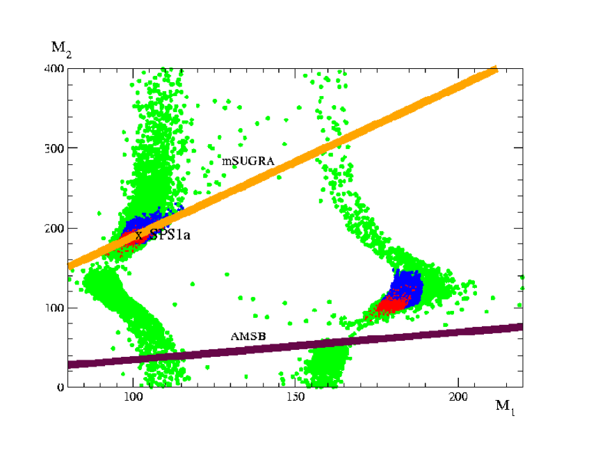
Figure 2: $M_{1}$, $M_{2}$ (in GeV units and at $Q_{EWSB}$ scale) determination from two (resp. three) neutralino masses $m_{\tilde{N}_{1}}$, $m_{\tilde{N}_{2}}$ ($m_{\tilde{N}_{4}}$) in unconstrained MSSM for different assumptions: 1) green regions: $m_{\tilde{N}_{1}}$, $m_{\tilde{N}_{2}}$ input, $\mu=\mu(\mbox{SPS1a})\pm 1$ TeV, $1\raisebox{-3.69899pt}{~{}\shortstack{$<$ \\ [-0.07cm] $\sim$}}~{}\tan\beta\raisebox{-3.69899pt}{~{}\shortstack{$<$ \\ [-0.07cm] $\sim$}}~{}50$; 2) blue regions: $m_{\tilde{N}_{1}}$, $m_{\tilde{N}_{2}}$ input, $1<\tan\beta<50$, $\Delta\mu=100$ GeV; 3) red regions: $m_{\tilde{N}_{1}}$, $m_{\tilde{N}_{2}}$ + $m_{\tilde{N}_{4}}$ input, $1\raisebox{-3.69899pt}{~{}\shortstack{$<$ \\ [-0.07cm] $\sim$}}~{}\tan\beta\raisebox{-3.69899pt}{~{}\shortstack{$<$ \\ [-0.07cm] $\sim$}}~{}50$ ($\mu$ is thus more constrained due to the third neutralino mass, see main text). Also shown are the mSUGRA or GMSB (resp. AMSB) $M_{1}/M_{2}$ relations in orange (respectively in maroon) including experimental errors on the masses.

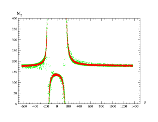
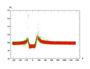
Figure 3: Correlated values of $M_{2}$ (left) and $M_{1}$ (right) for the $M_{1}<M_{2}$ case at $Q_{EWSB}$ scale as functions of $\mu$, for $m_{\tilde{N}_{1}},m_{\tilde{N}_{2}}$ input. The spreading of points is due to the variation $1<\tan\beta<50$ (in green) as well as the variation of $m_{\tilde{N}_{1}}$, $m_{\tilde{N}_{2}}$ within accuracy (in red).

The cases of moderate (blue region) and accurate (red region) determination of $\mu$ is giving much more interesting constraints. The red regions are anticipating the resulting accuracy on $\mu,M_{1},M_{2}$ when a third neutralino $m_{\tilde{N}_{4}}$ can be measured, as will be analyzed in a next subsection III.4. According to Eq. (13) in this case $\mu$ is determined (independently of $\tan\beta$) and can be combined with the previous Eqs. (10), (11) to obtain much improved $M_{1},M_{2}$ determination. (Alternatively another rather good determination of $\mu$ is also obtained when the latter is not arbitrary, as is assumed in a general MSSM, but calculated from EWSB consistency conditions from universal Higgs and sfermion mass terms at the GUT scale, as will be analyzed in section 6.) Now, contour plots like those in Fig. 2 are not very informative as concerns the improvement in $M_{1}$ or $M_{2}$ determination to be expected when increasing $\mu$ (or eventually $\tan\beta$) accuracies respectively. To trace more clearly this behaviour, we plot in Fig. 3 the equivalent of the green contour of Fig. 2 but in the $(\mu,M_{2})$ and $(\mu,M_{1})$ planes respectively (and for the $M_{1}<M_{2}$ case). (Note that the values of $M_{1}$ and $M_{2}$ are entirely correlated since both are obtained from Eqs. (54), 55)). The spreading of points in these plots is due to the variation of $\tan\beta$ and $m_{\tilde{N}_{1}}$, $m_{\tilde{N}_{2}}$. More precisely, what is shown in red in the effect of $m_{\tilde{N}_{1}}$, $m_{\tilde{N}_{2}}$ experimental errors only, for fixed SPS1a value of $\tan\beta=9.74$, while the additional green points correspond to $1<\tan\beta<50$. These plots are thus essentially the solutions $M_{1,2}(\mu)$ from Eqs. (54)-(55), that would reduce to simple curves for fixed $\tan\beta$, $m_{\tilde{N}_{1}}$, $m_{\tilde{N}_{2}}$. One can see the structure of solutions for $(M_{2},\mu)$ (and correspondingly $(M_{1},\mu)$) with different domains, originating from the $\mu$ dependence in Eqs. (55), with strong correlations. In fact $M_{2}(\mu)$ becomes arbitrarily large for two $\mu$ values, for $\mu<0$ and $\mu>0$ (which are not exactly symmetrical, see Appendix A): for instance for SPS1a values of $\tan\beta$, $m_{\tilde{N}_{1}}$, $m_{\tilde{N}_{2}}$, the positive “pole” is at $\mu\sim 118$ GeV. This explains the loose determination of $M_{2}$ for large variations of $\mu$, and also explains the density levels of scanned points in Fig. 2. In contrast, $M_{1}$ always remains finite when $M_{2}$ becomes arbitrary large, according to Eq. (54). This also explains the much better constraints on $M_{1}$ in Fig. 2 irrespectively of the $M_{2}$ behaviour.

Next, one can see that both $M_{2}$ and $M_{1}$ can be much better constrained, irrespectively of $\tan\beta$ values, as soon as the $\mu$ determination is slightly better (such that $\mu$ remains sufficiently far from these poles). This explains the much improved constraints on $M_{2}$ and $M_{1}$ for the blue contour in Fig. 2 (and a fortiori for the red contours where $\mu$ is tightly constrained from the third neutralino mass as will be discussed more in sub-sec. III.4). All these properties are rather simple consequences of the basic Eqs. (10)-(11), and illustrate useful informations that would be very difficult to delineate from a more standard top-down fit of parameters. Actually the poles for specific $\mu$ values are artifacts of our inversion equations, but more physically it simply means that to obtain precisely the $m_{\tilde{N}_{1}}$, $m_{\tilde{N}_{2}}$ SPS1a values for those particular $\mu$ values, $M_{2}$ would have to be unreasonably large. Going back to the standard top-down approach, it also means that performing e.g. a $\chi^{2}$ fit of the neutralino masses is likely to give a very flat behaviour of the $\chi^{2}$ near this $\mu$ region: more precisely, since $M_{2}$ varies widely around these $\mu$ values, no clear “best fit” $M_{2}$ value will be found, or with a very large error, and/or that the $\chi^{2}_{min}$ value will be bad. This is fully confirmed by the results of a MINUIT fit: if $\mu$ is fixed to $\sim 120$ GeV the minimization does not give useful constraints, MINUIT finds typically errors like:

$$M_{1}=2000\pm 258\;\mbox{GeV},\;\;M_{2}=2000\pm 88\;\mbox{GeV}\;.$$ (14)

with even many more minima and errors found for very large $M_{2}$ value.
In contrast, fixing $\mu$ (and $\tan\beta$) to their SPS1a values and fitting only $m_{\tilde{N}_{1}}$, $m_{\tilde{N}_{2}}$, gives very good accuracy on $M_{1},M_{2}$, as will be discussed in a next sub-section below where other MINUIT fit results are given (see Table 4):

$$M_{1}=108.8\pm 5.8\;\mbox{GeV},\;\;M_{2}=208.9\pm 6.4\;\mbox{GeV}\;.$$ (15)

Next, if gaugino mass universality at the GUT scale is assumed, as expected one obtains stronger constraints. This is illustrated on Fig. 2 by the (orange) band resulting from the “mSUGRA” relation: $M_{1}\simeq 0.53M_{2}$ at the low energy scale $Q\simeq Q_{EWSB}$, from $M_{1}(Q_{GUT})=M_{2}(Q_{GUT})$ at GUT scale. The width of this band results from the error on $M_{3}$, i.e. $m_{\tilde{g}}$ determination. We will see in next subsection how to make this study more precise when the (mSUGRA) gaugino mass universality is assumed. We anticipate, however, that for the given two neutralino and gluino mass accuracies, constraints on $\mu$ will be mild, even with gaugino mass universality assumptions, while those on $\tan\beta$ almost absent. Indeed, one can see on Fig. 2 that the “mSUGRA” band is compatible with a part of the green region where $\tan\beta$ (and $\mu$) are essentially undetermined.
Next, since the contours in Fig. 2 are valid for arbitrary gaugino masses, it is straightforward to superpose different gaugino mass relations, for instance in AMSBAMSB models where the $M_{1}/M_{2}$ relation is also fixed from high scale boundary conditions and RG evolution, but is very different: $M_{1}(Q_{EWSB})\simeq 2.9M_{2}(Q_{EWSB})$. We show similarly on Fig. 2 this ‘AMSB” band (in maroon) including its width originating from the $M_{3}$ uncertainty. In this way one may possibly distinguish, depending on the accuracy, between e.g. mSUGRA/GMSB and AMSB models from the neutralino mass measurements. (Note however that the relation between $M_{1}$ and $M_{2}$ in GMSB modelsGMSB is completely indistinguishable from the mSUGRA relation at this accuracy level). More precisely one can see here how AMSB would be excluded if moderate (in blue) or accurate (in red) $\mu$ measurements could be achieved (even when considering the second solution with $M_{1}>M_{2}$ which has an AMSB-like hierarchy pattern). This is also a consistency cross-check, in the present analysis, since we started from a mSUGRA model SPS1a “data”.

III.3 Reconstructing $\mu$, $\tan\beta$ with gaugino mass universality for SPS1a case

Let us now consider scenario S2 as discussed above, assuming gaugino mass universality Eq. (12) to determine $M_{1}$ and $M_{2}$, and next using basic Eqs. (10), (11) to determine $\mu^{2}$ and $\tan\beta$ for the SPS1a test case (see explicit solutions Eqs. (60), (61) in Appendix A). Numerically, for SPS1a, gaugino mass universality at GUT scale gives at the relevant low energy EWSB scale approximately:

$$M_{1}\simeq 0.17M_{3}\;,\;\;\;\;M_{2}\simeq 0.33M_{3}\;,\;\;\;M_{1}\simeq 0.53M_{2}\;.$$ (16)

To determine $M_{1}$, $M_{2}$ from $M_{3}$, we first extract $M_{3}$ from the the gluino pole mass $m_{\tilde{g}}$ as

$$m^{pole}_{\tilde{g}}=M_{3}(Q)+\Sigma_{\tilde{g}}(Q;m_{\tilde{q}},\cdots)$$ (17)

by subtracting out the leading radiative corrections $\Sigma_{\tilde{g}}$ to the gluino mass: those are dominantly due to squarks, and thus largely predictable in our framework, as discussed above in sub-section 2.3. This induces a non-negligible shift, since for SPS1a the correction $\Sigma_{\tilde{g}}\sim 20$ GeV, with $M_{3}(Q_{EWSB})\sim 600$ GeV.
As mentioned in sub-section III.1.2, The solutions of (10), (11) for $\tan\beta$ and $\mu$ do not determine the sign of $\mu$, so in the reconstruction with error propagation we have to consider the two possible solutions for $\mu>0$ and $\mu<0$. We first vary $M_{\tilde{g}}$, $m_{\tilde{N}_{1}}$, $m_{\tilde{N}_{2}}$ within accuracy according to Table 3. Scanning the values with (uniformly distributed) random numbers, with the conditions: $\mu$ real and $\tan\beta>0$, is illustrated in Figs. 4–6.

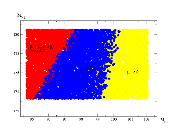
Figure 4: Allowed domain for $m_{\tilde{N}_{1}}$, $m_{\tilde{N}_{2}}$ corresponding to complex or real $\mu$.

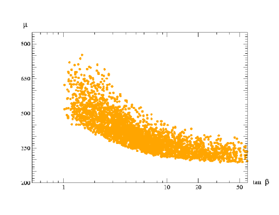
Figure 5: Constraints on $\mu>0$, $\tan\beta$ from gaugino universality and gluino plus two neutralino mass measurements in gluino cascade decay.

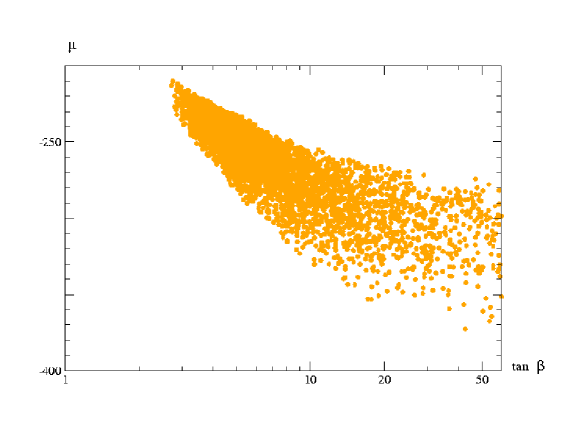
Figure 6: Constraints on $\mu<0$, $\tan\beta$ (at $Q_{EWSB}$ scale) from gaugino universality and gluino plus two neutralino mass measurements in gluino cascade decay.

A number of remarks are worth here: first, requiring $\mu$ to be real further reduces the errors on neutralino masses, since the red domain in Fig. 4 is to be excluded. In the most general MSSM case, $\mu$ may have a non-zero phase, but if we restrict our analysis to a real parameter space, this is an interesting additional constraint, resulting solely from the consistency of Eqs. (10), (11). The two other domains correspond to $\mu>0$ and $\mu<0$ respectively, so that the latter cannot be excluded given these SPS1a accuracies on the two neutralino masses. We notice that if neutralino mass accuracies could be reduced by a factor of about 2, the $\mu<0$ solution would disappear altogether (as well as the complex $\mu$ possibility).

Next the corresponding constraint in the $\tan\beta,\mu$ plane are shown in Figs. 5 and 6 respectively for $\mu>0$ and $\mu<0$. We observe that $\tan\beta$ is practically unconstrained, especially for large $\tan\beta$, and $\mu>0$ poorly constrained, for these accuracies on neutralino and gluino masses. However for $\mu>0$ the two parameters appear strongly correlated, as shown by the contour shape: e.g. for $\mu>0$, large $\mu\sim 600-700$ GeV is only possible for small $\tan\beta\sim 2$. This correlation is not an artifact of our simple random scan, but a simple consequence of the $\mu$ and $\sin 2\beta$ dependence within Eqs. (10), (11) (see explicitly Eq. (62) in Appendix A). Note also that the sign of $\mu$ and of $\sin 2\beta$ are partly correlated (see Eq. (62), so that our convention $\tan\beta>0$ impose constraints that are quite different for the $\mu>0$ and $\mu<0$ cases. More precisely we find:

$$\tan\beta\raisebox{-3.69899pt}{~{}\shortstack{$>$ \\ [-0.07cm] $\sim$}}~{}1\;,\;\;\;280\>\mbox{GeV}\raisebox{-3.69899pt}{~{}\shortstack{$<$ \\ [-0.07cm] $\sim$}}~{}\mu\raisebox{-3.69899pt}{~{}\shortstack{$<$ \\ [-0.07cm] $\sim$}}~{}750\>\mbox{GeV}$$ (18)

for $\mu>0$ and

$$\tan\beta\raisebox{-3.69899pt}{~{}\shortstack{$>$ \\ [-0.07cm] $\sim$}}~{}2.7\;,\;\;\;210\>\mbox{GeV}\raisebox{-3.69899pt}{~{}\shortstack{$<$ \\ [-0.07cm] $\sim$}}~{}|\mu|\raisebox{-3.69899pt}{~{}\shortstack{$<$ \\ [-0.07cm] $\sim$}}~{}370\>\mbox{GeV}$$ (19)

for $\mu<0$, and in both cases no upper limits on $\tan\beta$, which is simply understandable because only $\sin 2\beta$ appears in any of the relations above in Eqs. (9–11), so that for large $\tan\beta$ any sensitivity on $\tan\beta$ disappears.

These results are thus consistent with what was anticipated from the previous analysis illustrated in Fig. 2, where the gaugino “mSUGRA” universality band is crossing all domains of the chosen $\tan\beta,\mu$ range of variation: in particular the green region where $\tan\beta$ was essentially arbitrary. The fact that $\mu$ is better constrained for $\mu<0$ is understandable from Fig. 4 where the domain corresponding to $\mu<0$ is smaller than the $\mu>0$ one, moreover the central value $|\mu|\sim 357$ GeV is excluded on the plot Fig. 6 This is due to the partly correlated sign of $\mu$ and $\sin 2\beta$ in this inverted determination (see Eq. (62)), but without knowing the true SPS1a value of $\mu$ we could not exclude $\mu<0$ solutions solely from these cascade decay mass accuracies.

III.4 Scenario S3: $\mu$, $\tan\beta$ from three neutralino with or without universal gaugino masses

Let us finally consider another (more optimistic) scenario S3 where three neutralino masses could be determined according to the input $S_{3}$ in Table 1 above. As explained above in this case one gets from Eqs. (9) an extra relation, Eq. (13), resulting in a determination of $\mu$ independent of $\tan\beta$, which is valid both for the general MSSM case, or assuming additional gaugino mass relations (like universal ones typically). For the general MSSM, the much improved determination of $M_{1},M_{2}$ was illustrated by the red domains in Fig. 2. Here for completeness we illustrate in Fig. 7 the corresponding domains in the $(M_{1},\mu)$ planes, for the two possible case $M_{1}<M_{2}$ (in orange) corresponding to SPS1a, and also for the alternative solution with $M_{2}<M_{1}$ (in red). $|\mu|$ is determined with an accuracy of about $\Delta\mu\sim 15$ GeV, but as already mentioned the sign of $\mu$ remains undetermined. Moreover, in a most general MSSM, without any prior knowledge on gaugino and Higgsino mass relative values, the sole knowledge of three neutralino masses does not determine the relative hierarchy among $M_{1}$, $M_{2}$, and $|\mu|$. So strictly speaking there is a six-fold ambiguity in this case, considering all possible ordering of these three parameters (see Appendix A).

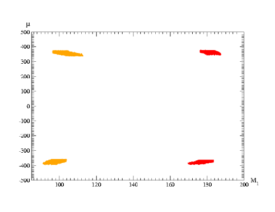
Figure 7: Constraints on $M_{1}$, $\mu$ (at $Q_{EWSB}$ scale) in general MSSM for three neutralino mass measurements in gluino + squark cascade decay.

We now consider the gaugino mass universality case with three neutralino mass input. The ambiguity on the relative magnitude of $M_{1}$, $M_{2}$ and $\mu$ obtained in a general MSSM is of course resolved in this case since the hierarchy at the low scale is entirely determined from universal initial values of $M_{i}$. The resulting constraints on $\mu,\tan\beta$ are illustrated in Fig. 8, where one observes that the $\mu<0$ solution has disappeared (and the equivalent of Fig. 4 would show that only a smaller part of the red contour $\mu>0$ is surviving). However, only $\mu$ is much more constrained, while apart from a slightly more interesting lower bound, $\tan\beta$ remains essentially unconstrained for large $\tan\beta$. This is simply due to the $\sin 2\beta$ only dependence in all these relations, whatever the number of input neutralino masses. More precisely:

$$\tan\beta\raisebox{-3.69899pt}{~{}\shortstack{$>$ \\ [-0.07cm] $\sim$}}~{}2.7\;,\;\;\;350\>\mbox{GeV}\raisebox{-3.69899pt}{~{}\shortstack{$<$ \\ [-0.07cm] $\sim$}}~{}\mu\raisebox{-3.69899pt}{~{}\shortstack{$<$ \\ [-0.07cm] $\sim$}}~{}372\>\mbox{GeV}\;.$$ (20)

These results are consistent with general expectations, namely that the gaugino sector alone can hardly constrain $\tan\beta$ at the LHC, even in the mSUGRA (gaugino universality) case, but these features are perhaps very simply illustrated here analytically.

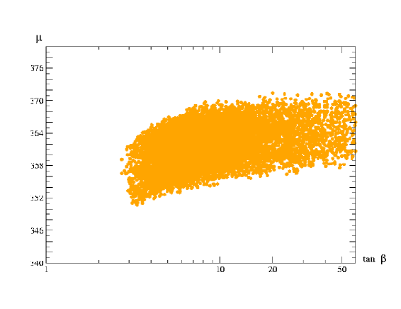
Figure 8: Constraints on $\mu$, $\tan\beta$ from gaugino universality and gluino plus three neutralino mass measurements in gluino + squark cascade decay.

Concerning the inclusion of radiative corrections into this essentially tree-level determination, we have already mentioned the use of the $\overline{DR}$ parameters $\bar{s}^{2}_{W}$, $\bar{m}_{Z}$ in all these relations, which already incorporates a part of the corrections. The bulk of these $\overline{DR}$ corrections with respect to tree-level values come from standard model contributions, and supersymmetric contributions, though not negligible, are strictly speaking inducing some theoretical uncertainties if loop contributions from unknown sector are taken into account. Next, the corrections from the running to the pole neutralino masses remain moderate in the MSSM, so that one may neglect them in a first approximation. Actually, most of these radiative corrections can be incorporated in the form of corrections to the “bare” parameters $\mu$, $M_{1}$, $M_{2}$ to very good approximationbpmz , while additional corrections in the neutralino mass sector are smallerbpmz . Our procedure to determine e.g. $M_{1}$, $M_{2}$ or $\mu$ above remains thus correct, up to an implicit shift on these parameters, provided that one has some knowledge on these radiative corrections. In fact gluino mass corrections are dominantly due to squarks/quark, and quite similarly for neutralinos, so they can be evaluated within a reasonable approximation, without assuming more knowledge than the available cascade decay input. Though it is not completely straightforward to incorporate consistently all these corrections within these parameters, it is very similar to the kind of iterative procedure required for a standard top-down calculation of MSSM spectrumsuspect , as discussed in sub-section 2.3. This is taken into account in the above illustrations.

Table 4: Constraints on gaugino-Higgsino sector parameters (at $Q_{EWSB}$ scale) from a standard top-down $\chi^{2}$ MINUIT fit of neutralino and gluino masses under different universal or non-universal gaugino mass assumptions.

Data $\&$ fitted parameter	MIGRAD ($68\%$C.L.)	MINOS ($68\%$C.L.)	nominal
(+ model assumptions)			SPS1a value
$m_{\tilde{N}_{1}},m_{\tilde{N}_{2}},m_{\tilde{g}}$	(convergent)	(problems)
(Non-universal $M_{i}$;
1-loop RGE; no $\tilde{N}_{i}$ R.C.)
$M_{1}$	$\sim$97–126 (from fit)		108.8
$M_{2}$	$\sim$181–381 (from fit)		208.9
$\mu$	200–1500 (scanned)		340.6
$\tan\beta(Q_{EWSB})$	1–50 (scanned)		9.74
$m_{\tilde{N}_{1}},m_{\tilde{N}_{2}},m_{\tilde{N}_{4}},m_{\tilde{g}}$	(convergent)	(convergent)
$M_{1}$	108.8 $\pm 7.2$	108.8 $\pm 7.2$	108.8
$M_{2}$	208.9 $\pm 8.2$	208.9 $\pm 8.2$	208.9
$\mu$	340.6 $\pm 11.6$	340.6 $\pm 11.6$	340.6
$\tan\beta(Q_{EWSB})$	9.74 (fixed)	9.74 (fixed)	9.74
$m_{\tilde{N}_{1}},m_{\tilde{N}_{2}},m_{\tilde{g}}$	(convergent)	(problems with $\tan\beta$)
(Universal $M_{i}(Q_{GUT})$;
1-loop RGE; no $\tilde{N}_{i}$ R.C.)
$M_{3}$	603.8 $\pm 13.5$	603.8 $\pm 13.5$	603.8
$\mu$	341.6 $\pm 293$	341.6 $\pm 293$	340.6
$\tan\beta(Q_{EWSB})$	9.73 $\pm 52.6$	(not calculated)	9.74
$m_{\tilde{N}_{1}},m_{\tilde{N}_{2}},m_{\tilde{N}_{4}},m_{\tilde{g}}$	(convergent)	(problems with $\tan\beta$)
$M_{3}$	603.8 $\pm 13.4$	603.8 $\pm 13.4$	603.8
$\mu$	340.6 $\pm 13$	340.6 $\pm 13$	340.6
$\tan\beta(Q_{EWSB})$	10.0 $\pm 15.3$	(not calculated)	9.74

In order to cross-check the inverse analytical determination above, we perform alternatively standard top-down $\chi^{2}$ minimization fits, using MINUIT. The best fit results, with or without gaugino mass universality assumptions and for different assumptions on $\mu$ and $\tan\beta$, are shown in Table 4 both for two and three neutralino mass input. Actually, in the non-universal gaugino mass case, two neutralino masses are clearly not enough input to constrain the four parameters $M_{1}$, $M_{2}$, $\mu$ and $\tan\beta$. Thus to compare as much as possible with the previous reconstruction results, in this case we also perform scans over $\mu$ and $\tan\beta$ (taking $\mu\raisebox{-3.69899pt}{~{}\shortstack{$>$ \\ [-0.07cm] $\sim$}}~{}200$ GeV to avoid the pole region discussed above). The corresponding results obtained for the “envelope” of best fit values, with confidence level domains for $M_{1}$ and $M_{2}$, are shown in the second column of Table 4 (in the first two entries). The rather bad constraints obtained in this case are roughly consistent with the above analysis of the $\mu$ dependence of $M_{2}$ and $M_{1}$ illustrated in Fig. 2, and already discussed above. (Note that our simple top-down fit is not able to exhibit the $M_{1},M_{2}$ reconstruction ambiguities in the non-universal gaugino mass case, discussed in sub-sec. 3.1, 3.4 and Appendix A, though these ambiguities may be implicitly responsible for the large errors found for $M_{1}$, $M_{2}$, when $\mu$ is varied in a wide range). Similar ambiguities are however more clearly exhibited when performing more sophisticated minimization, where typically extra “best fit solutions” appeardzerwas ). In contrast, the determination of $M_{1}$, $M_{2}$ is much improved if $\mu$ is better constrained, and accordingly there is a substantial improvement on the $\mu$ determination if the third neutralino mass input $m_{\tilde{N}_{4}}$ is available, as shown in the Table. Those results from Table 4 are thus roughly consistent with the analytic behaviour illustrated in Figs. 3, 7, and 8. The symmetrical (MIGRAD) minimization, however, does not reflect very well the true sensitivity to some of the parameters, most notably for $\tan\beta$. Indeed the unsymmetrical non-linear MINOS minimization does not give any useful constraint for $\tan\beta$, even for universal gaugino mass assumptions. Note that in the latter case $m_{\tilde{N}_{1}},m_{\tilde{N}_{2}}$ are essentially Bino-like and Wino-like respectively, while $m_{\tilde{N}_{4}}$ is essentially Higgsino-like, which also explain the drastic improvement on $\mu$ accuracy from a third neutralino mass input.

III.5 Reconstructing gaugino masses at GUT scale

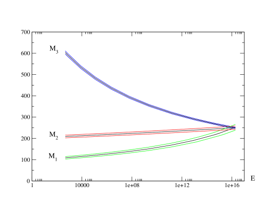
Figure 9: Bottom-up RGE of gaugino masses from EWSB to GUT scale, including error propagations ($\mu$ and $\tan\beta$ are fixed to their SPS1a values).

Finally we perform a bottom-up RGE of the gaugino mass parameters in the non-universal case, in order to check eventually for their unification at a high GUT scale, following ref. bpzm123 . (NB the bottom-up RGE procedure for gaugino masses and other basic MSSM parameters from given values at EWSB scale is explained in Appendix B). This is first shown in Fig. 9, taking the best $M_{i}(Q_{EWSB})$ determination above (i.e. corresponding to three neutralino mass input), and in Fig. 10 taking the worst $M_{i}(Q_{EWSB})$ determinations (i.e. a scenario with two neutralino mass input and no known constraints on $\mu$). One can see that a very good check of GUT scale universality is possible as long as the initial $M_{i}(Q_{EWSB})$ accuracies are reasonable: in other words, the error dispersion from the gaugino mass RGE remains small (which is clearly explained from the fact that their RGE content only depend on gauge couplings at the one-loop level). As expected this is qualitatively consistent with the former results of ref. bpzm123 (though it appears that the $M_{1}$, $M_{2}$ LHC accuracies considered at that time were slightly more optimistic than the ones we obtain here from our analysis). Note that the dispersion due to the bottom-up RGE can be much more important for other parameter sectors, in particular for the $m_{H_{u}}$ parameter in the Higgs sector (see the discussion in Appendix B). Nevertheless, the possibility of checking universality at GUT scale may become elusive even for gaugino masses in the extreme case where almost nothing is known on $\mu$, such that the $M_{1}$, $M_{2}$ low scale values errors are large. In this case only the $M_{3}$ error remains under control, as illustrated in Fig. 10. We also remark once more that in addition to performing a bottom-up RGE, mSUGRA gaugino universality could be checked efficiently from plots as illustrated in Fig. 2 (where it can also be eventually distinguished from other high scale SUSY-breaking models like AMSB).

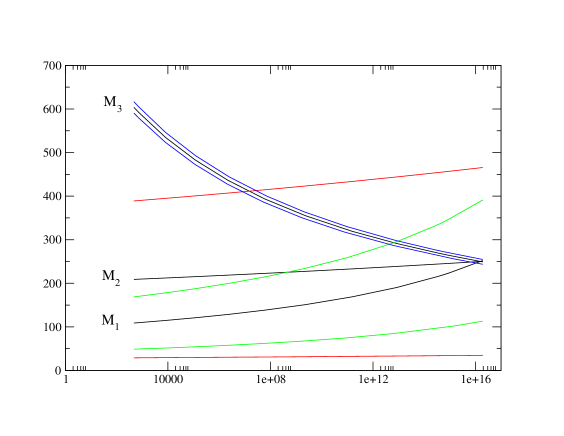
Figure 10: Bottom-up RGE of gaugino masses from EWSB to GUT scale, including error propagations for the worst case ($\mu$ and $\tan\beta$ undetermined).

IV Squark/slepton parameter determination (first two generations)

We now consider a bottom-up reconstruction approach for the (first and second generation) squark and/or slepton sector parameter of the MSSM. Because of the negligible mixing for the first and second generations, as well as the simplified RGE structure of this sector, we can elaborate a rather general strategy to reconstruct the relevant parameters up to an (eventual) GUT scale. Similarly to the gaugino/Higgsino sector, we shall consider two different model assumptions: a general MSSM sfermion sector, or a more constrained scenario assuming universality of slepton and squark masses.

IV.1 General MSSM and a simple squark/slepton mass sum rule

The masses of the sfermions $\tilde{q}(\neq\tilde{b},\tilde{t})$ and $\tilde{l}$ which participate to the cascade decay in Eq. (1) obey (at the EWSB scale) well-known relations (at tree-level) e.g for the up squark and selectron:

$$m^{2}_{\tilde{u}_{1}} = m^{2}_{\tilde{u}_{L}}+(\frac{1}{2}-\frac{2}{3}s^{2}_{W})m^{2}_{Z}\cos 2\beta$$

$$m^{2}_{\tilde{e}_{2}} = m^{2}_{\tilde{e}_{R}}-s^{2}_{W}m^{2}_{Z}\cos 2\beta$$ (21)

which are valid in the general MSSM . Similar relations hold for the other squark and slepton flavors. Eqs. (21) simply relate the physical masses to the soft breaking scalar masses via the additional D-terms. These relations are particularly simple for the first two squark and slepton generations due to negligible mixing. The main idea is to consider specific linear combination (“sum rules”) in order to eliminate the $\tan\beta$ dependence:

$$s_{W}^{2}m_{\tilde{u}_{1}}^{2}+(\frac{1}{2}-\frac{2}{3}s_{W}^{2})m_{\tilde{e}_{2}}^{2}=s_{W}^{2}{m_{\tilde{u}_{L}}^{2}}+(\frac{1}{2}-\frac{2}{3}s_{W}^{2}){m_{\tilde{e}_{R}}^{2}}\;.$$ (22)

Then taking into account the available accuracy on the physical masses $m_{\tilde{u}_{1}}$ and $m_{\tilde{e}_{2}}$ provides constraints on the MSSM soft-breaking scalar parameters $m_{\tilde{u}_{L}},m_{\tilde{e}_{R}}$ independently of $\tan\beta$ values. So, even if $\tan\beta$ is largely undetermined (as is the case from the neutralino sector alone at LHC, illustrated in previous section), Eq. (22) gives a (model-independent) determination of the linear combination of basic parameters which will be roughly of the order of magnitude of the physical mass accuracies, i.e. a few percent for typical LHC prospects. More precisely, a straightforward calculation from the experimental accuracy in Table 3 gives a $\sim 2.3\>\%$ ($\sim 2\>\%$) relative accuracy for the linear combination in Eq. (22), if we combine the $m_{\tilde{u}_{1}}$ and $m_{\tilde{e}_{2}}$ errors linearly (quadratically), respectively. (NB we have neglected at the moment for simplicity the error on $\bar{s}^{2}_{W}$: the effect of $\bar{s}^{2}_{W}$ uncertainties will be studied below). Another advantage of this linear combination is that, even in a general non-universal MSSM case, the RG evolution of the relevant parameters ($m_{\tilde{u}_{L}}(Q)$, $m_{\tilde{e}_{R}}(Q)$) depends only on the gauge couplings $g_{i}$ and the gaugino masses $M_{i}$ . The linear combination Eq. (22) can thus be RG-evolved within a restricted set of input parameters solely determined from the gluino cascade, in order to obtain the soft scalar term values at the GUT scale, where one may check for eventual universality relations. Before doing this RG evolution, it is necessary to subtract out radiative corrections linking the running to the pole masses, which are not negligible for squarks, in the way discussed in section 2.3. More precisely we have

$$M^{pole}_{\tilde{u}_{1}}=m_{\tilde{u}_{1}}(Q)+\Delta m_{\tilde{u}_{1}}(Q,m_{\tilde{q}},m_{\tilde{g}},...)$$ (23)

where these corrections are largely dominated by squark/gluino contributions at one-loop. For a typical mSUGRA scenario like SPS1a we have $\Delta m_{\tilde{u}_{1}}(Q_{EWSB},m_{\tilde{q}},m_{\tilde{g}})\sim 19$ GeV, which can be consistently subtracted out to define the running mass $m_{\tilde{u}_{1}}$. Concerning radiative corrections linking the running to the pole slepton mass, they are generally much smaller and we shall neglect them in our analysis.
Next, it is a straightforward exercise to work out the RG evolution of the linear combination (22):

$$\frac{d}{dt}\left[s_{W}^{2}{m_{\tilde{u}_{L}}^{2}}+(\frac{1}{2}-\frac{2}{3}s_{W}^{2}){m_{\tilde{e}_{R}}^{2}}\right]= s^{2}_{W}\frac{dm^{2}_{\tilde{u}_{L}}}{dt}+(\frac{1}{2}-\frac{2}{3}s_{W}^{2})\frac{dm^{2}_{\tilde{e}_{R}}}{dt}$$ (24)

$$+\frac{ds^{2}_{W}}{dt}(m^{2}_{\tilde{u}_{L}}-\frac{2}{3}m^{2}_{\tilde{e}_{R}})$$

where $t\equiv\ln Q$ and the standard RG evolution of the relevant parameters $\tilde{m}^{2}_{u_{L}}$, $\tilde{m}^{2}_{e_{R}}$ is used (which as mentioned only depend on $g_{i}$, $M_{i}$). We also have:

$$\frac{ds^{2}_{W}}{dt}=(\frac{3}{5}g^{2}_{1}+g^{2}_{2})^{-1}\>\left(\frac{3}{5}c^{2}_{W}\frac{dg^{2}_{1}}{dt}-s^{2}_{W}\frac{dg^{2}_{2}}{dt}\right)$$ (25)

with $s^{2}_{W}(t)\equiv\frac{3}{5}g^{2}_{1}(t)/(\frac{3}{5}g^{2}_{1}(t)+g^{2}_{2}(t))$ and the factor $3/5$ is due to the standard normalization of the $U(1)_{Y}$ coupling $g_{1}$ in the MSSM RGE. Eqs. (24) and (25) take into account the RG evolution of $\bar{s}^{2}_{W}$. (Note that the latter is not at all negligible since it is related to the running of gauge couplings, which change substantially from $m_{Z}$ input values to GUT scale values).

As already mentioned one important feature of this bottom-up RG evolution is that some of the low scale parameter uncertainties are amplified once evolved to a large scale, depending on the structure of RG beta functions for some of the relevant parameters: this is the case to some extent with the evolution of Eq. (22, as we will see later.

IV.2 Constrained MSSM with squark, slepton universality

If we now assume squark and slepton mass universality at the GUT scale, Eq. (24) immediately determines $m^{q,l}_{0}(Q_{GUT})$:

$$s_{W}^{2}{m_{\tilde{u}_{L}}^{2}}+(\frac{1}{2}-\frac{2}{3}s_{W}^{2}){m_{\tilde{e}_{R}}^{2}}(Q_{GUT})\equiv\frac{5}{8}\>(m^{q,l}_{0})^{2}$$ (26)

where the gauge coupling universality relation at the GUT scale: $s^{2}_{W}(t=\ln Q_{GUT})=3/8$ has been used. $m^{q,l}_{0}$ indicates that we only assume universality for the (first two generation) squark and slepton sector at this stage, i.e. not necessarily for the third generation sfermions, nor for Higgs scalar terms like in mSUGRA models.

IV.3 Explicit reconstruction test for the SPS1a input

We now determine explicit constraints on the squark and/or slepton sector parameters from the specific SPS1a blind input with the expected accuracy on the masses of $\tilde{q}_{L}$ and $\tilde{l}_{R}$ from Table 3. As already mentioned in section 2, there is at present no way to tag the charge and flavor of the relevant (first two generations) squark at LHC. Accordingly the resulting mass accuracies of say, an up or down squark, are assumed to be identicalcascade2 , so that there is no need to combine their errors in a statistically elaborated manner, and we thus assume that it is sufficient for our purpose to take the average of two (identical) errors in our analysis. By combining thus the accuracies on the measured $\tilde{u}_{1}$ and $\tilde{e}_{2}$ masses in Table 3, we obtain for SPS1a from Eqs (22), (26):

$$84\>(86)\>\mbox{GeV}\raisebox{-3.69899pt}{~{}\shortstack{$<$ \\ [-0.07cm] $\sim$}}~{}m^{q,l}_{0}\raisebox{-3.69899pt}{~{}\shortstack{$<$ \\ [-0.07cm] $\sim$}}~{}116\>(112)\>\mbox{GeV}\;.$$ (27)

Note that the first limits are for linearly combined mass uncertainties (while those in parenthesis are for quadratically combined mass uncertainties). We emphasize that the bounds in Eq. (27) are independent of $\tan\beta$ values. However, there is a rather important amplification of the initial low scale uncertainty $\sim 2\%$ due to error propagation in the bottom-up RG evolution, and because of the additional terms proportional to $ds^{2}_{W}/dt$ in Eq. (24). To better trace the origin of the resulting $m_{0}$ uncertainties, it is illustrative to consider independently the squark and slepton mass uncertainties: this gives

$$86.6\>\mbox{GeV}\raisebox{-3.69899pt}{~{}\shortstack{$<$ \\ [-0.07cm] $\sim$}}~{}m^{q,l}_{0}(\Delta m_{\tilde{u}_{1}})\raisebox{-3.69899pt}{~{}\shortstack{$<$ \\ [-0.07cm] $\sim$}}~{}112\>\mbox{GeV}$$ (28)

and

$$97.1\>\mbox{GeV}\raisebox{-3.69899pt}{~{}\shortstack{$<$ \\ [-0.07cm] $\sim$}}~{}m^{q,l}_{0}(\Delta m_{\tilde{e}_{2}})\raisebox{-3.69899pt}{~{}\shortstack{$<$ \\ [-0.07cm] $\sim$}}~{}103\>\mbox{GeV}$$ (29)

respectively. Thus the final uncertainty on $m_{0}$ is largely dominated by the $m_{\tilde{u}_{1}}$ initial accuracy. Actually, the latter bounds on $m^{q,l}_{0}$ were calculated while fixing the gaugino mass terms $M_{i}$. But since the RG evolution of $m_{\tilde{u}_{L}},m_{\tilde{e}_{R}}$ depends on gaugino masses, the $m^{q,l}_{0}$ accuracy should be sensitive to $M_{i}$ uncertainties, mainly those of $M_{3}$ which are enhanced in the $m_{\tilde{u}_{L}}$ RGE by the strong coupling: $dm^{2}_{\ u_{L}}/dt\sim-\frac{8}{3\pi}\alpha_{S}M^{2}_{3}$rge ; RGE2 . This leads to an important amplification of $m^{q,l}_{0}$ final uncertainty due to the $\Delta M_{3}\sim 7$ GeV uncertainty (although the latter effect is damped somehow by $\bar{s}^{2}_{W}\sim.238$ in the first term of the RHS of Eq. (24), while other terms in Eq. (24) are not much sensitive to $M_{i}$ uncertainties). One thus obtains, in the conservative case of uncorrelated and linearly combined errors, a maximal uncertainty on $m^{q,l}_{0}$ of about $\pm\sim 32$ GeV (respectively $\pm\sim 22$ GeV when combining errors quadratically) instead of the bounds shown in Eqs. (27)–(29) . However, the linear combination Eq. (22) does not use the full information from the two independent mass relations in Eq. (21): we shall illustrate below how this additional information improves rather substantially the limits on $m^{q,l}_{0}$.

Another potentially interesting question is whether one can derive at the same time any useful limits on $\tan\beta$, once using the complete information from both squark and slepton masses. At first sight one may naively expect to obtain some upper bounds on $\tan\beta$, since the relations (21) are sensitive to $\cos 2\beta$. However a simple estimate immediately indicates that interesting $\tan\beta$ upper bounds from this squark, slepton sector are hardly expected for the given LHC $\tilde{e}_{2},\tilde{u}_{1}$ mass accuracies: in fact for the SPS1a point with $\tan\beta(Q_{EWSB})\sim 9.74$, $\cos 2\beta\sim-0.979$ i.e. very close to $-1$, so that one would need at least an accuracy $\raisebox{-3.69899pt}{~{}\shortstack{$<$ \\ [-0.07cm] $\sim$}}~{}0.02$ on $|\cos 2\beta|$ to put useful upper limits on $\tan\beta$. In contrast, a simple calculation of uncertainties from both Eqs. (21) gives:

$$\Delta|\cos 2\beta|\sim 0.6$$ (30)

even in the optimistic case where we combine the $m_{\tilde{u}_{1}},m_{\tilde{e}_{2}}$ uncertainties quadratically, and neglect the errors on $s^{2}_{W}$. The above estimate, however, does not take into account other possible constraints on $\tan\beta$, that may come from other sectors, or from theoretical consistency. For instance the obvious constraint: $|\cos 2\beta|\leq 1$ puts additional limits on $m^{2}_{e_{R}}-m^{2}_{\tilde{e}_{2}}$ via Eqs. (21), so indirectly on $m^{q,l}_{0}$. Furthermore, for $m^{q,l}_{0}\sim 100$ GeV it is easily checked that $\tan\beta$ cannot be larger than $\tan\beta\raisebox{-3.69899pt}{~{}\shortstack{$<$ \\ [-0.07cm] $\sim$}}~{}35-36$, since beyond this value the lightest stau $m_{\tilde{\tau}_{1}}$ mass becomes tachyonic due to the large stau mixing $\bar{m}_{\tau}\,.\mu\tan\beta$ term. Moreover, the lightest Higgs mass becomes inconsistent (or too low) for small $\tan\beta\raisebox{-3.69899pt}{~{}\shortstack{$<$ \\ [-0.07cm] $\sim$}}~{}2.2$ approximately, and for low $\tan\beta$ values the LEP lower bounds on $m_{h}$LEPmh actually put a tighter constraint $\tan\beta\raisebox{-3.69899pt}{~{}\shortstack{$>$ \\ [-0.07cm] $\sim$}}~{}8-9$. Yet the latter limits are theoretical and model-dependent (or experimental and model-dependent in the case of $m_{h}$ bounds), and specific of the SPS1a benchmarkbenchmark , which was chosen on purpose to satisfy the present experimental constraints. If we push $m^{q,l}_{0}$ sufficiently above the SPS1a central values, the upper bound $\tan\beta\raisebox{-3.69899pt}{~{}\shortstack{$<$ \\ [-0.07cm] $\sim$}}~{}35$ from tachyonic $\tilde{\tau}_{1}$ is easily evaded, though in this case one should also take into account the lower bound $m_{\tilde{\tau}}\raisebox{-3.69899pt}{~{}\shortstack{$>$ \\ [-0.07cm] $\sim$}}~{}104$ GeV from LEP limitsLEPlim . (For example, for $m_{0}\sim 200$ GeV $\tan\beta\sim 50$ is not excluded by tachyonic stau, while the gluino, squarks cascade decays would not be drastically different from the SPS1a one). Similarly, the $\tan\beta$ lower bound due to LEP $m_{h}$ lower limits could easily be evaded in an unconstrained MSSMadkps . We will thus not apply such direct (or indirect) experimental limits which are much dependent on the specific SPS1a choice, since our main aim is to present a reconstruction strategy expected to be valid beyond this particular benchmark choice.

Accordingly a question that we examine in some detail next is whether the sole $m_{\tilde{u}_{1}},m_{\tilde{e}_{2}}$ mass measurements could put some extra model-independent limits on $\tan\beta$. From the previous estimate it appears that to obtain stringent such experimental constraints on $\tan\beta$, one would require an accuracy about an order of magnitude better on the squark and slepton masses than the one prospected at the LHC. Incidentally this is roughly the accuracy expected at the ILC (though only for the sleptons), where both $l_{R}$ and $l_{L}$ masses could be measured at the per mille levelLHCstudy ; SPA . However, a detailed ILC analysis is beyond the scope of the present paper and left for future work.
We anticipate that (model-independent) limits on $\tan\beta$ will be indeed absent, or very marginal if using solely the first two generation squark and slepton mass accuracies. This is consistent with general prospectsLHCstudy ; kane . We found however useful to examine this issue in some detail, since our construction is not limited to the LHC mass accuracies here considered: thus tracing analytically the sensitivity on parameters can help to understand better what determines the constraints in a more elaborated analysis.

To begin, there is a subtlety that is not taken into account in the above crude estimate of error combination in Eq. (30), such that it may underestimate the $\tan\beta$ sensitivity: as emphasized previously the RG equations for $m_{\tilde{u}_{L}},m_{\ e_{R}}$ only depend on gauge couplings and gaugino masses, so in particular do not depend on $\tan\beta$ (at one-loop level). But there is in fact an indirect dependence on $\tan\beta$ even at one-loop (though very moderate): it originates from the boundary conditions on the RGE, namely the initial values of gauge couplings $g_{i}$ in the $\overline{DR}$ scheme, as well as their values at the GUT scale (if gauge unification is imposed), depend slightly on $\tan\beta$ through radiative corrections (see e.g. ref. bpmz ). Although these effects are strictly speaking small higher order corrections on $g_{i}(m_{Z}),g_{i}(m_{GUT})$ values, they are enhanced when running parameters from low to high GUT scale over more than 13 orders of magnitude. Indeed most realistic calculations of MSSM spectra do take into account this dependence consistentlyisasugra ; softsusy ; spheno ; suspect . Also, these values are notoriously different if using the RGE at the full two-loop level, or in a one-loop approximation, as will be illustrated below. (This is somewhat similar to the impact of precise initial gauge couplings and RGE approximations on the GUT scale value $\sim 2\times 10^{16}$ GeV).

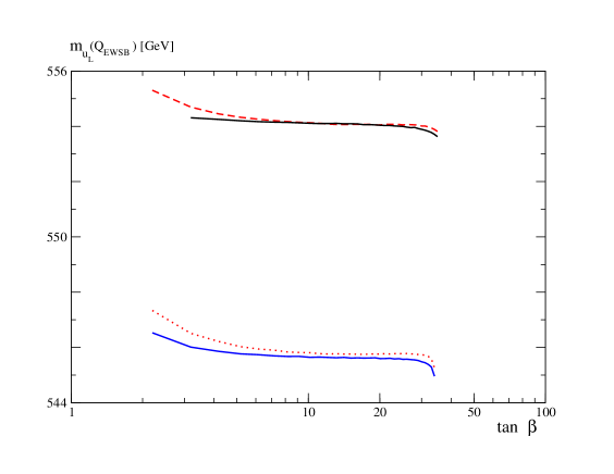
Figure 11: $m_{\tilde{u}_{L}}(Q_{EWSB})$ as function of $\tan\beta$ for SPS1a in one-loop RGE (top plots) and two-loop RGE (bottom plots). Red dashed line: one-loop RGE, default $Q_{EWSB}=(m_{\tilde{t}_{1}}m_{\tilde{t}_{2}})^{1/2}$. Black line: fixed $Q_{EWSB}=468$ GeV. Orange dotted line: two-loop RGE, defeat $Q_{EWSB}=(m_{\tilde{t}_{1}}m_{\tilde{t}_{2}})^{1/2}$. Blue line: fixed $Q_{EWSB}=468$ GeV.

Moreover, the low energy EWSB scale at which all soft parameters are evaluated also depend in principle on $\tan\beta$ values, and more generally it is not fixed by first principles: in most analysis the default EWSB scale is often fixed to $Q_{EWSB}\sim(m_{\tilde{t}_{1}}m_{\tilde{t}_{2}})^{1/2}$ (which is know to minimize the scale dependenceVscale of the MSSM one-loop effective scalar potential). For the SPS1a point this is a well-defined value, but when relying only on the gluino cascade decay data, the stop masses are not assumed to be know in a general MSSM case. Thus we can in principle vary this EWSB scale, which can affect the final value of soft scalar masses, since this scale determines the endpoint of the RG evolution. In our calculation we use either a fixed value (close to the true SPS1a for definiteness), or adopt the above default value in universality cases. In fact $m_{\tilde{u}_{L}}$ is expected to be specially sensitive to such variations, due to the large coefficient $\sim\alpha_{S}M^{2}_{3}$ within its RGE, which makes it to run much faster than $m_{\tilde{e}_{R}}$. (E.g. for SPS1a $m_{\tilde{u}_{L}}(Q_{GUT})=100$ GeV evolves to $m_{\tilde{u}_{L}}(Q_{EWSB})\sim 560$ GeV.)

For illustration in Fig. 11 we vary $m_{\tilde{u}_{L}}(Q_{EWSB})$ as function of $\tan\beta$, at one- and two-loop RGE order, both with fixed and default EWSB scale, using SuSpect 2.41. The variation with $\tan\beta$ is less than 2 GeV for $m_{u_{L}}$ (and we checked that it is completely negligible for $m_{e_{R}}$) for the whole $\tan\beta$ theoretically allowed range. This is accordingly below the prospected LHC accuracy on $m_{\tilde{u}_{L}}$, and thus rather negligible for our analysis. In contrast, there is a large difference between one and two-loop RGE, but this is usually the case for the whole MSSM spectrum, as it is well known. This illustrates that for such reconstruction (or in fact any other reconstruction methods) one should be careful to be consistent with the RGE approximation used. Concerning now the small $\tan\beta$ dependence it should be kept in mind that any more elaborated fit (as could be performed from a $\chi^{2}$ minimization using MINUIT) will be eventually sensitive to such effects, since these cannot be easily “switched off” from the fitting procedure. Moreover, such indirect dependence on $\tan\beta$ will be relevant anyway once reaching a better accuracy on slepton masses as is prospected at the ILC.

All these features are examined more quantitatively from a systematic scan over parameters, where we took into account the propagation of $m_{\tilde{u}_{1}},m_{\tilde{e}_{2}}$ uncertainties in both relations (21) after evolving from low to high scale, and back. More precisely we scanned over allowed mass bounds, considering the two mass uncertainties as independent (and uncorrelated) for simplicity. We also took into account any additional small dependence e.g. on $\tan\beta$ such as the one illustrated in Fig. 11. The ($m^{q,l}_{0},\tan\beta$) distributions obtained are shown first in Fig. 12 (the scan was performed with $3000$ uniformly distributed random numbers).

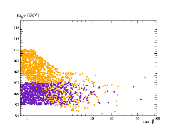
Figure 12: Constraints on $m_{0}\equiv m^{q,l}_{0}(Q_{GUT})$ and $\tan\beta$ from first two generation squark and slepton in gluino cascade decays after bottom-up RG evolution. The orange (respectively magenta) points correspond to constraints obtained from the squark $m_{\tilde{u}_{1}}$ (respectively $m_{\tilde{e}_{2}}$) relations in Eqs. (21).

Comparing with Eq. (27) one notes that the lowest values of $84\raisebox{-3.69899pt}{~{}\shortstack{$<$ \\ [-0.07cm] $\sim$}}~{}m_{0}\raisebox{-3.69899pt}{~{}\shortstack{$<$ \\ [-0.07cm] $\sim$}}~{}94$ GeV have been excluded simply from the constraint $|\cos 2\beta|<1$. However, arbitrary large values of $\tan\beta$ are possible (provided that a sufficiently large number of scan points are taken), confirming the simple error estimate above in Eq. (30). The fact that large values of $\tan\beta$ are very few in Fig. 12, while low $\tan\beta$ values appear very much favored, is actually an artifact of the (uniform) scanning procedure where we basically scanned over the $m_{\tilde{u}_{1}}$, $m_{\tilde{e}_{2}}$ masses, which determine $\cos 2\beta$ via Eq. (21) rather than $\tan\beta$. So the distribution of points in Fig. 12 is simply resulting from the transformation from $\cos 2\beta$ to $\tan\beta$ and has not much statistical meaning as “most likely” values of $\tan\beta$. As already mentioned we shall refrain to enter into a fully realistic statistical treatment of uncertainties, which would require to take into accountdzerwas , among other things, the non-trivial correlations implied by the cascade decay mass measurements. It is yet tempting in the present case to proceed one step further with a little more elaborated analysis. We thus perform a different scan, where instead of uniformly distributed “flat prior” random numbers, we exploit simple trigonometric relations to match more faithfully the true $\tan\beta$ distribution. In addition we start with Gaussian-distributed random numbers (assuming thus that the two independent errors are purely statistical, which is actually not really correctcascade1 ; cascade2 ). We then calculate a “theoretical” $\chi^{2}$ (where $\chi^{2}_{min}=0$ trivially since we use the correct central values of the masses) just to obtain well-defined confidence levels (C.L.) for the (joint) estimation of the two parameters $m^{q,l}_{0}$ and $\tan\beta$, assumed to be independent and uncorrelated.

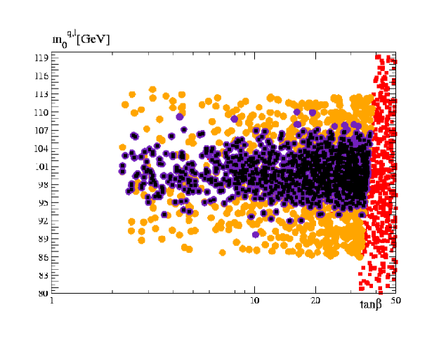
Figure 13: Constraints on $m_{0}\equiv m^{q,l}_{0}(Q_{GUT})$ and $\tan\beta$ with a scan over Gaussian random numbers: orange disks: 2-$\sigma$ allowed points ($\chi^{2}=\chi^{2}_{min}+6$) from $m_{\tilde{e}_{2}}$ relation; indigo disks: 2-$\sigma$ allowed points from $m_{\tilde{u}_{1}}$ relation; black squared: 1-$\sigma$ allowed points ($\chi^{2}=\chi^{2}_{min}+2.3$) from $m_{\tilde{u}_{1}}$ relation. Red squared: excluded by tachyon $\tilde{\tau}_{1}$. (NB the square or disk sizes have no physical meaning).

The result of this Gaussian scan is shown in Fig. 13. The domains obtained from the $m_{\tilde{e}_{2}}$ and $m_{\tilde{u}_{1}}$ relations in Eq. (21), at one-$\sigma$ level (more precisely $68\%$ C.L.) are shown in black, and the additional points allowed at two-$\sigma$ ($95\%$) C.L. are shown in indigo and orange respectively. The distribution of those allowed points is now essentially uniform in $\tan\beta$ (though now the apparent concentration for relatively large $\tan\beta$ is purely an artifact of the logarithmic scale), in contrast with the previous plot in Fig. 12. More importantly, $\tan\beta$ is constrained by lower and upper bounds, but these essentially originate from the theoretical (model-dependent) constraints, indicated in red for large $\tan\beta$ which correspond to a tachyon $\tilde{\tau}_{1}$. (NB the white zone for $\tan\beta\raisebox{-3.69899pt}{~{}\shortstack{$<$ \\ [-0.07cm] $\sim$}}~{}2.2$ corresponds to a very light $m_{h}$). More precisely we observe that even at the $68\%$ C.L., values of $\tan\beta$ up to the theoretical SPS1a constraint $\tan\beta\raisebox{-3.69899pt}{~{}\shortstack{$<$ \\ [-0.07cm] $\sim$}}~{}35$ are not excluded. Moreover one sees that the $95\%$ C.L. additionnal points (indigo and orange) have only the effect of slightly enlarging the $m^{q,l}_{0}$ determination but not much influence on the $\tan\beta$ determination. Thus a more realistic treatment of errors simply confirms our above crude estimate, indicating that no interesting model-independent upper limits on $\tan\beta$ can be derived from the prospected LHC squark and slepton masses accuracies.

It is instructive to compare at this stage those results with a more standard top-down fit. We thus used MINUIT to perform a standard $\chi^{2}$ minimization starting from a MSSM model with universal GUT $m^{q,l}_{0}$ and $\tan\beta$ free parameters. First we fix the gaugino masses $M_{1},M_{2},M_{3}$ to their SPS1a values and then fit this model to the “data” consisting solely of $m_{\tilde{u}_{1}},m_{e_{2}}$. This two-parameter fit result is shown in Table 5 for different MINUIT minimization options, at the one-$\sigma$ level.

Table 5: Constraints on $m_{0},\tan\beta$ obtained from a standard top-down $\chi^{2}$ fit with different model and input assumptions and different level of MINUIT minimizations.

Data $\&$ fitted parameter	MIGRAD	MINOS	nominal
(+ model assumptions)	minimization ($68\%$C.L.)	minimization ($68\%$C.L.)	SPS1a value
$m_{\tilde{e}_{2}},m_{\tilde{u}_{1}}$
(1-loop RGE + no $\tilde{q}$ R.C.)	(convergent)	$\tan\beta$ exceed limits
$m^{q,l}_{0}$	99.98 $\pm 8.8$	99.98 $\pm$ 8.7	100
$\tan\beta$	9.41 $\pm$ 29.8	9.41 ${}^{+\mbox{\small no limits}}_{-\mbox{\small no limits}}$	9.74
$m_{\tilde{e}_{2}},m_{\tilde{u}_{1}}$ +
$m_{\tilde{N}_{1}},m_{\tilde{N}_{2}},m_{\tilde{g}}$
(1-loop RGE + no $\tilde{q}$ R.C)	(convergent)	$\tan\beta$ exceed limits
$m^{q,l}_{0}$	99.96 $\pm 7.9$	99.9 ${}^{+10}_{-10.5}$	100
$m_{1/2}$	250 $\pm 4.3$	250 $\pm 4.3$	250
$\tan\beta$	10. $\pm$ 29.8	10 ${}^{+29.8}_{-\mbox{\small no limits}}$	9.74

In fact the simpler MIGRADminuit (symmetric error) minimization did converge, giving apparently a (marginal) upper $\tan\beta$ limit at the one-$\sigma$ level. But it is not a very useful $\tan\beta$ bound, being above the theoretical $\tan\beta$ limits in this SPS1a case. Moreover, the more elaborated MINOS minimization, taking into account properly unsymmetrical errors and non-linearitiesminuit , did not find any $\tan\beta$ upper (nor lower) limits. These results are thus qualitatively consistent with our more naive analysis above. Note that the $m_{0}$ bounds are also roughly consistent with our previous results. Now there are several reasons not to trust even the marginal upper bounds found for $\tan\beta$: though it is difficult to trace the very details of the minimization steps, the fit is much probably indirectly influenced by the $\tilde{\tau}_{1}$ becoming very small (and ultimately tachyonic) for $\tan\beta\raisebox{-3.69899pt}{~{}\shortstack{$>$ \\ [-0.07cm] $\sim$}}~{}35-36$. More precisely, above those values, SuSpect still gives $m_{\tilde{u}_{1}}$, $m_{\tilde{e}_{2}}$ output (unless explicit warning flags are switched on), but these are no longer very reliable (because the iterations needed to calculate a convergent spectrum are stopped in this casesuspect ). In particular, there is an abrupt change of $m_{\tilde{u}_{L}}$ once $\tan\beta\raisebox{-3.69899pt}{~{}\shortstack{$>$ \\ [-0.07cm] $\sim$}}~{}36$, see Fig. 11 (though the overall variation remains reasonable). Thus, comparing these minimization results and Fig. 13 with the simple estimate Eq. (30), we can infer that the marginal upper bound on $\tan\beta$ is principally determined by the indirect small higher order $\tan\beta$ dependences (like typically the dependence $m_{\tilde{u}_{L}}(\tan\beta)$ as illustrated in Fig. 11 originating mainly from the slightly varying EWSB scale, rather than directly from the $m_{\tilde{u}_{1}}$, $m_{\tilde{e}_{2}}$ accuracies). We have crosschecked this by redoing similar fits with a constant EWSB scale, or with two-loop RGE, which both have the effect of smoothing somehow the variation of $m_{\tilde{u}_{L}}(\tan\beta)$ near the transition to tachyonic $\tilde{\tau}_{1}$ for $\tan\beta\sim 36$, and the $\tan\beta$ upper bound in Table 5 tends to increase (or even to disappear with non convergent minimizations). We have also further checked this by increasing progressively the mass accuracies: while the corresponding $m_{0}$ bounds decrease, following the expected statistical behaviour, for $\tan\beta$ one obtains either non convergent minimizations, or extra odd solutions far from the SPS1a values. There are anyway no improvements on $\tan\beta$ bounds until a substantial decrease of these experimental errors is set (about an order of magnitude smaller than the LHC accuracies of Table 3).

For completeness we performed another minimization, taking into account in addition the neutralino and gluino masses with a three-parameter fit of $m_{0},m_{1/2},\tan\beta$. The situation does not improve much as concerns $\tan\beta$ limits, as illustrated by the corresponding results in Table 5. In this case the (unsymmetrical) MINOS $m_{0}$ bounds are slightly worse than for the two-parameter fit, which is expected since now $M_{3}$ is not fixed. Accordingly the $M_{3}$ accuracy propagates to the $m_{0}$ determination via the RGE, as explained above. On the other hand the accuracy on $m_{1/2}$ is very good. Finally we also performed a similar fit for a benchmark point like SPS1a except $m_{0}=200$ GeV, in which case the transition to tachyonic $m_{\tilde{\tau}_{1}}$ happens only for very large $\tan\beta>50$, having thus potentially less influence on the fit. Assuming the same mass accuracies than for the true SPS1a point we obtain, for a two-parameter (respectively three-parameter) fit: $\tan\beta=9.93\pm 52.2$ (respectively $\tan\beta=10.1\pm 50.7$), at one-$\sigma$ level, while errors for $m_{0}$ and $m_{1/2}$ are very comparable to the SPS1a ones. So this confirm the above analysis and indicates that the $\tan\beta$ upper bounds are essentially inexistent.

This also illustrates that a “global” top-down fit, whatever elaborated with MINUIT algorithms, may be fooled and lead to misleading conclusions due to extra parameter dependences which originate from theoretical approximation artifacts (e.g. here the choice of EWSB scale, RGE approximation, etc). In the present case, one could of course easily avoid such problems by simply adding protections within the minimization procedure, but that would amount to put explicitly the (model-dependent) upper bound on $\tan\beta$ due to tachyonic (or more generally too light) $\tilde{\tau}_{1}$.

We finally examine two questions related to theoretical uncertainties that are relevant to the above analysis. First, as already mentioned in deriving the $m^{q,l}_{0}$ constraints in Eqs. (27-28) we had neglected for simplicity the errors on $s^{2}_{W}$: the latter are actually not quite negligible, since even a small uncertainty can in principle affect our determination from Eq. (22). However, the bulk of radiative correction contributions to the $\bar{s}^{2}_{W}$ parameter, in the $\overline{DR}$ scheme, originates from standard model and are thus predictable in our framework. Additional supersymmetric contributions are not negligible eitherbpmz , but we checked that varying all MSSM parameters and sparticle masses form the SPS1a to models with arbitrary MSSM values produces a variation of $\bar{s}^{2}_{W}$ of about $0.6\%$ only. One may probably push parameters to extreme values to find a slightly larger variation, so we conservatively consider a $1\%$ uncertainty on $\bar{s}^{2}_{W}$. The impact on $m_{0}$ determination is an (upper) shift by about $\sim 3$ GeV with respect to the numbers quoted in Eqs. (27-28). Note that the correct dependence of $m_{0}$ and $\tan\beta$ upon $\bar{s}^{2}_{W}$ is automatically taken into account in the MINUIT fit results in Table 5.

Another potential question is that the determination of $m^{q,l}_{0}$ via Eq. (22) together with RGE, depends only on the cascade masses if restricting the RGE to one-loop order. At the two-loop order, practically all other MSSM parameters are entering the RGE. Nevertheless, it is possible to study the impact of this uncertainty by assuming, within the two-loop RGE level, simple (e.g. universal) relations for the unknown parameters, and to redo our analysis: while central values are evidently shifted, the impact on error propagation is rather negligible, with minor quantitative changes on e.g. the obtained $m^{q,l}_{0}$ constraints. This is also consistent with some comparisons we made of two-loop versus one-loop RGE fit results using MINUIT.

We thus conclude that $\tan\beta$ is essentially unconstrained from the data we used at this stage, which is not much a surprise and consistent with general expectations on LHC prospectsLHCstudy ; kane . Model-independent constraints on $\tan\beta$, though moderate, may be obtained however from other sectors as we shall see in next sections, either considering the information from bottom squarks in the cascade, or adding the lightest Higgs mass measurements.

V Third generation squark parameter determination

We will now consider the possible determination of some of the third generation squark parameters. As discussed in section 2, the sbottoms enter the gluino cascade and both mass eigenstates may be measured to some extent (though with less accuracy for the heaviest $\tilde{b}_{2}$)LHCstudy ; cascade2 . We will examine what additional information they provide, both in unconstrained MSSM or assuming universality relations, as in previous analyses.

V.1 Scenario S5: constraints from the sbottom masses in non-universal MSSM

So far, we have obtained from the gluino cascade useful constraints on the gaugino/Higgsino parameters and $m^{q,l}_{0}$, while $\tan\beta$ is very poorly determined. The sbottom sector may provide information on the missing third generation soft scalar terms, or eventually on $\tan\beta$. To set up signs and other conventions, we recall the sbottom mass squared matrix:

$$M_{\tilde{b}}^{2}=\left(\begin{array}[]{cc}{m^{2}_{Q3L}}+m_{b}^{2}+(-\frac{1}{2}+\frac{1}{3}s^{2}_{W})\,m^{2}_{Z}\cos 2\beta&m_{b}\,({A_{b}}-\mu\tan\beta)\\ m_{b}({A_{b}}-\mu\tan\beta)&{m_{b_{R}}^{2}}+m_{b}^{2}-\frac{1}{3}\,m^{2}_{Z}\cos 2\beta\end{array}\right)$$ (31)

where again all parameters are implicitly understood to be in the $\overline{DR}$ scheme. It is immediate that the trilinear term $A_{b}$ will be very badly determined, being largely suppressed by the bottom mass $m_{b}$, with $\bar{m}_{b}(Q_{EWSB})\sim 3$ GeV e.g. in SPS1a, and similar values in more general SUSY scenarios. However, this also means that we can practically neglect $A_{b}$. In this case the sbottom masses determine, to a good approximation, the third generation parameters $m_{Q3_{L}}$, $m_{b_{R}}$ in a simple way directly from (the trace of) (31):

$$m^{2}_{\tilde{b}_{1}}+m^{2}_{\tilde{b}_{2}}+\frac{m^{2}_{Z}}{2}\cos 2\beta-2m^{2}_{b}\equiv S=m^{2}_{Q3_{L}}+m^{2}_{b_{R}}\;.$$ (32)

Now, taking one of the mass eigenvalue (say $m_{\tilde{b}_{1}}$) as a given function of the other parameters $\mu,\tan\beta$ etc, we can solve a simple relation for $m_{Q3_{L}}$, $m_{b_{R}}$:

$$m_{Q3_{L}(b_{R})} = \left[\frac{S+(-)D}{2}\right]^{1/2}$$

$$D = -Y+\left[(m^{2}_{\tilde{b}_{2}}-m^{2}_{\tilde{b}_{1}}-2m_{b}X_{b})(m^{2}_{\tilde{b}_{2}}-m^{2}_{\tilde{b}_{1}}+2m_{b}X_{b})\right]^{1/2}\;,$$ (33)

where $Y=(-\frac{1}{2}+\frac{2}{3}s_{W}^{2})m^{2}_{Z}\cos 2\beta$ and $X_{b}=A_{b}-\mu\tan\beta$. There is in fact a twofold ambiguity, namely a second solution where $m_{Q3_{L}}\leftrightarrow m_{b_{R}}$ in Eq. (33), since it is a second order equation. For SPS1a we know that $m_{Q3_{L}}(Q_{EWSB})>m_{b_{R}}(Q_{EWSB})$ resolves this ambiguity, but for unconstrained MSSM one has to deal in principle with the two possibilities in the absence of further information other than the sbottom masses. In addition one also expects radiative corrections to this tree-level determination which might spoil its simplicity. Radiative corrections to sbottom masses are not negligible in general, but to a very good approximation they are largely dominated by gluino and squark contributions, as already discussed in sub-section 2.3. So we have a reasonable knowledge of these corrections, such that the running masses in the $\overline{DR}$ scheme involved in Eqs (33) may be obtained from the pole masses after appropriate subtractions.

V.2 Explicit reconstruction: SPS1a test case

The resulting $m_{Q3_{L}}$, $m_{b_{R}}$ determination for the SPS1a test case with corresponding input mass accuracies is illustrated in Fig. 14. We plot the allowed range for $m_{Q3_{L}}$, $m_{b_{R}}$ obtained from a (uniform) scan over mass accuracies from Table 3 and the other relevant parameters, as indicated. Different cases are illustrated when varying $\tan\beta$ and $\mu$ within the previously obtained limits, i.e. $\mu\sim 360\pm 200$, or more constrained situations, $\Delta\mu\pm 10$ (the latter corresponding roughly to the case where three neutralino masses can be measured), and $3\raisebox{-3.69899pt}{~{}\shortstack{$<$ \\ [-0.07cm] $\sim$}}~{}\tan\beta\raisebox{-3.69899pt}{~{}\shortstack{$<$ \\ [-0.07cm] $\sim$}}~{}35$ (using the theoretical upper bound for SPS1a). Since $A_{b}$ is essentially unknown at this stage, we vary it widely in the range: $-1$ TeV to $1$ TeV.

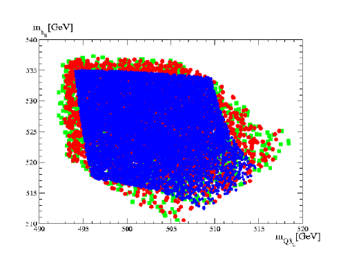
Figure 14: Constraints in general MSSM on $m_{Q3_{L}}$, $m_{b_{R}}$ (at $Q_{EWSB}$ scale) from $m_{\tilde{b}_{1}},m_{\tilde{b}_{2}}$ measurements in the gluino cascade decays. Radiative corrections linking the pole to running masses have been subtracted out. Experimental errors on sbottom masses are taken from Table 3. Blue region: fixed nominal values of $\tan\beta\sim 9.74$, $\mu\sim 357$ GeV (and $A_{b}=0$). Red region: $3\raisebox{-3.69899pt}{~{}\shortstack{$<$ \\ [-0.07cm] $\sim$}}~{}\tan\beta\raisebox{-3.69899pt}{~{}\shortstack{$<$ \\ [-0.07cm] $\sim$}}~{}35$, $\Delta\mu\sim 10$ GeV, $-100GeV<A_{b}<100GeV$; green region: $3\raisebox{-3.69899pt}{~{}\shortstack{$<$ \\ [-0.07cm] $\sim$}}~{}\tan\beta\raisebox{-3.69899pt}{~{}\shortstack{$<$ \\ [-0.07cm] $\sim$}}~{}50$, $\Delta\mu\sim 200$ GeV, $-1\mbox{TeV}<A_{b}<1\mbox{TeV}$. Nominal SPS1a values are $m_{Q3_{L}}=503$ GeV, $m_{b_{R}}=525$ GeV (at one-loop RGE level).

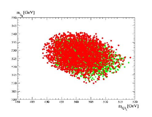
Figure 15: Comparison of uniform (in green) versus Gaussian (in red) scan with one-$\sigma$ ($68\%$ C.L.) level contours. The variation of extra parameters correspond to the less determined range in Fig. 14, i.e.: $3\raisebox{-3.69899pt}{~{}\shortstack{$<$ \\ [-0.07cm] $\sim$}}~{}\tan\beta\raisebox{-3.69899pt}{~{}\shortstack{$<$ \\ [-0.07cm] $\sim$}}~{}50$, $\Delta\mu\sim 200$ GeV, $-1\mbox{TeV}<A_{b}<1\mbox{TeV}$.

As one can see, the determination of $m_{Q3_{L}}$, $m_{b_{R}}$ is quite accurate even in a non-universal MSSM case, and for largely unknown $A_{b}$. This is clearly explained by the strong suppression of $A_{b}$, which has thus practically no influence on the scalar mass parameter determination. Moreover, the variation of $\mu$, and even the large variation of $\tan\beta$, have no strong influence either, which is explained by the fact that they are both very suppressed also by $m_{b}$ as compared to other parameters. To examine the impact of radiative corrections, we did a similar scan but neglecting on purpose the radiative corrections, i.e. using as central values the pole sbottom masses. As a result the $m_{Q3_{L}}$, $m_{b_{R}}$ central values are substantially shifted with respect to nominal SPS1a values, but the accuracy obtained on $m_{Q3_{L}}$, $m_{b_{R}}$ is very similar.

Next, in Fig. 15 we compare the previous results obtained from a simple scan with uniformly distributed random number with those from a scan made with Gaussian-distributed random numbers, defining a $\chi^{2}$ domain similarly to the analysis in section 4. One can see that the corresponding one-$\sigma$ limits show the expected statistical behaviour, having a more regularly-shaped contour than the one in the uniform case, but with no drastic changes in the limits obtained on $m_{Q3_{L}}$, $m_{b_{R}}$.

V.3 Scenario $S^{\prime}_{5}$: constraints from sbottoms in MSSM with sfermion mass universality

Prospects for the third generation scalar terms are better in a more constrained MSSM i.e. with universality relations assumed in the scalar sector. In this case, one has:

$$m^{q,l}_{0}\equiv m_{Q3_{L}}(Q_{GUT})=m_{b_{R}}(Q_{GUT})$$ (34)

Then, using the above results from section 4 on $m^{q,l}_{0}$ limits, one can determine from a top-down RGE the corresponding accuracy obtained on $m_{Q3_{L}}(Q_{EWSB})$ and $m_{b_{R}}(Q_{EWSB})$:

$$m_{Q3_{L}}(Q_{EWSB})\sim 498\pm 1.2\pm 7\mbox{GeV},\;\;\;m_{b_{R}}(Q_{EWSB})\sim 521\pm 1.8\pm 6\mbox{GeV}\;,$$ (35)

where the first errors correspond to a variation of $m_{0}$ for fixed $M_{3}$, while the second additional errors take into account the $m_{\tilde{g}}\sim M_{3}$ uncertainty (which dominates the final uncertainties). Alternatively, one may use here the limits on $m_{0}$ obtained from the $\chi^{2}$ minimization in Table 5, which would gives results roughly comparable to the bounds in Eq. (35) (except that it is somewhat more difficult to disentangle the effect of the $M_{3}$ uncertainties from the fit). Comparing with the unconstrained MSSM determination from the sbottom masses in Figs. 14, 15 one can see a definite improvement on $m_{Q3_{L}}(Q_{EWSB})$ and $m_{b_{R}}(Q_{EWSB})$ accuracies by about a factor two. This may be sufficient to resolve the twofold ambiguity between $m_{Q3_{L}}$ and $m_{b_{R}}$ discussed above in the non-universal sfermion case.

Perhaps more interestingly, one may expect to derive an independent determination of $\tan\beta$ in this sfermion universality scenario, by combining all information from $m_{0}$ and the sbottom masses. More precisely, turning the other way round Eqs. (33) one can determine very simply $X_{b}=Ab-\mu\tan\beta$ in terms of the know parameters, as follows:

$$2\,m_{b}\,X_{b}=-\left[(m^{2}_{\tilde{b}_{2}}-m^{2}_{\tilde{b}_{1}})^{2}-(m^{2}_{\tilde{Q}3_{L}}-m^{2}_{\tilde{b}_{R}}+Y)^{2}\right]^{1/2}.$$ (36)

(Actually Eq. (36) comes from a second order equation, so in principle there is again a twofold ambiguity: $2m_{b}X_{b}=\pm[\cdots]^{1/2}$. But within our sign convention, if $\mu>0$, $X_{b}<0$ necessarily, even for general MSSM, unless $|\mu|\tan\beta<A_{b}$, which is not a very common situation except perhaps for very small $\tan\beta$ values.) 

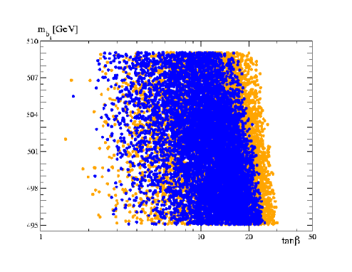
Figure 16: Constraints on $\tan\beta$ with uniform scan from $m_{\tilde{b}_{1}},m_{\tilde{b}_{2}}$ accuracies. $A_{b}$ is assumed to be almost undetermined ($A_{b}=A_{b}(\mbox{SPS1a})\pm 1$ TeV). In blue : $\Delta m_{\tilde{b}_{2}}=7.9$ GeV. In orange: $\Delta m_{\tilde{b}_{2}}=16$ GeV.

The resulting determination of $X_{b}$ and $\tan\beta$ from Eq. (36) is first illustrated in Fig. 16: while $X_{b}$ is directly determined from Eq. (36), for $\tan\beta$ one has to take into account the additional uncertainties in the determination of $\mu$ (and $A_{b}$, which is assumed to be essentially unknown at this stage). However it is clear that this has a moderate impact on the $\tan\beta$ determination, since even a large variation $-1\>\mbox{TeV}<A_{b}<1\>\mbox{TeV}$ has a moderate effect, $\sim\Delta A_{b}/\mu$ (unless if $|\mu|$ would be very small). So even at this stage where $A_{b}$ is completely undetermined, reasonable constraints: $\tan\beta\raisebox{-3.69899pt}{~{}\shortstack{$<$ \\ [-0.07cm] $\sim$}}~{}27-28$ are obtained, as shown by the blue contour. Moreover, even when increasing the $m_{\tilde{b}_{2}}$ uncertainty by a factor of two, i.e. $\Delta m_{\tilde{b}_{2}}\sim 16$ GeV, one still obtains some reasonable constraints on $\tan\beta\raisebox{-3.69899pt}{~{}\shortstack{$<$ \\ [-0.07cm] $\sim$}}~{}30$, see Fig. 16. (But the upper bound on $\tan\beta$ disappear if the $\tilde{b}_{2}$ is not measured at all). Like for the previous section analysis, we also show the difference between uniform and Gaussian scans, with corresponding one- and two-$\sigma$ contours in Fig. 17. For completeness the joint (correlated) determination of $(\tan\beta,X_{b})$ is also shown in Fig. 18.

We thus observe that, provided the two sbottom masses can be measured with this accuracy at the LHC, the bounds on $\tan\beta$ may start to be rather interesting, at least at the one-$\sigma$ level. These results are also confirmed by a $\chi^{2}$ minimization fit using MINUIT, with more or less comparable bounds obtained, as shown in Table 6.

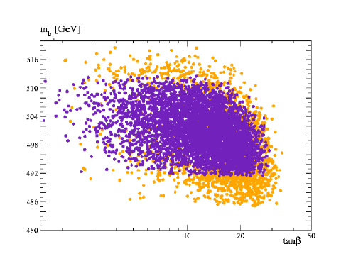
Figure 17: Constraints on $\tan\beta$ from Gaussian scan: indigo: one-$\sigma$ ($68\%$ C.L.); in orange: two-$\sigma$ ($95\%$ C.L.).

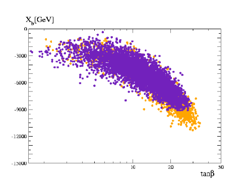
Figure 18: Constraints on $\tan\beta,X_{b}=A_{b}-\mu\tan\beta$ from Gaussian scan: indigo: one-$\sigma$ ($68\%$ C.L.); orange: two-$\sigma$ ($95\%$ C.L.).

Table 6: Constraints on $m_{0},\tan\beta$ obtained from a standard top-down $\chi^{2}$ fit of squark +sbottom masses and neutralino/gluino masses, for different options of MINUIT minimizations.

Data $\&$ fitted parameter	MIGRAD	MINOS	nominal
(+ model assumptions)	minimization ($68\%$C.L.)	minimization ($68\%$C.L.)	SPS1a value
$m_{\tilde{e}_{2}},m_{\tilde{u}_{1}}$, $m_{\tilde{b}_{1},b_{2}}$ +
$m_{\tilde{N}_{1}},m_{\tilde{N}_{2}},m_{\tilde{g}}$
(1-loop RGE + no $\tilde{q}$ R.C)	(convergent)	$\tan\beta$ exceed limits
$m^{q,l}_{0}$	99.96 $\pm 9.9$	99.9 ${}^{+10}_{-10.4}$	100
$m_{1/2}$	250 $\pm 3.6$	250 $\pm 3.6$	250
$\tan\beta(m_{Z})$	9.98 $\pm$ 13.6	9.98 ${}^{+13.6}_{-\mbox{\small no limits}}$	10

We finally mention that squark and slepton universality relations as in Eq. (34) is yet not enough to have any interesting determination of $A_{b}$, which is quite obvious from its very suppressed contribution to the mass matrix (31). One thus needs a different strategy to determine, if possible, the remaining trilinear couplings. The prospects for the latter would be certainly much better if one could measure the stop masses in similar cascades. This is not the case for the SPS1a, but we will examine in the next section how the Higgs sector parameters can help to determine the stop sector trilinear couplings.

VI Bottom-up reconstruction of Higgs sector parameters

In the Higgs sector, the most relevant parameters (at tree-level) are the scalar mass terms $m_{H_{u}}$, $m_{H_{d}}$ and $\tan\beta$. These may be replaced equivalently, using the EWSB conditions, by $\mu$, the pseudoscalar mass $m_{A}$, and $\tan\beta$. More precisely, the EWSB minimization equations $\partial V_{\rm Higgs}/\partial H_{d}=0$; $\partial V_{\rm Higgs}/\partial H_{u}=0$ (where $V_{\rm Higgs}$ designates the MSSM scalar potential) can be solved for $\mu^{2}$ and $B\mu$:

$$\mu^{2} = \frac{1}{2}\left[\tan 2\beta(m^{2}_{H_{u}}\tan\beta-m^{2}_{H_{d}}\cot\beta)-m_{Z}^{2}\right]$$

$$B\mu = \frac{1}{2}\sin 2\beta\left[m^{2}_{H_{u}}+m^{2}_{H_{d}}+2\mu^{2}\right]$$ (37)

which eventually includes radiative corrections to the scalar potential in the form of tadpole corrections $t_{u}$, $t_{d}$ potential ; bpmz :

$$m^{2}_{H_{u}}\to m^{2}_{H_{u}}-t_{u}/v_{u}\ {\rm and}\ m^{2}_{H_{d}}\to m^{2}_{H_{d}}-t_{d}/v_{d}\;.$$ (38)

Next, the running $m_{A}(Q)$ is defined as:

$$\bar{m}^{2}_{A}(Q)=m^{2}_{H_{d}}(Q)+m^{2}_{H_{u}}(Q)+2\mu^{2}(Q)$$ (39)

(where as previously all parameters are implicitly understood to be in the $\overline{DR}$ scheme). The $A$ pole mass is then related to $m_{A}(Q)$ via additional radiative correctionsmh1-2loop ; bpmz . It is well-known, however, that in the MSSM the scalar top sector contributes largely to radiative corrections to $m_{h}$ and $m_{A}$. Thus even if some parameters are available from other sector analysis (though not precisely for $\tan\beta$ as we have seen), only an independent measurement of $m_{A}$ (or alternatively an information on the stop sector, on $X_{t}\equiv A_{t}-\mu/\tan\beta$) could give a more useful information on the remaining parameters. For the determination of these Higgs parameter sector in a general (non-universal) MSSM case, the prospects are thus not very good if the available data are similar to those of the SPS1a benchmark, even if the lightest Higgs mass $m_{h}$ could be determined with a good accuracy. In a constrained MSSM with complete high scale universality of scalar soft terms, prospects are possibly better. We can then use our previous analysis with in addition:

$$m^{q,l}_{0}\equiv m_{H_{u}}(Q_{GUT})=m_{H_{d}}(Q_{GUT})$$ (40)

to determine $\mu$ via Eqs. (VI) as well as the running $m_{A}$ value in Eq. (39). From Eq. (VI) one has very roughly for $\tan\beta\gg 1$: $\mu^{2}\sim-m^{2}_{H_{u}}$ which is largely insensitive to $\tan\beta$. (NB in our analysis we use of course the complete expressions from Eqs. (VI)). Thus the rather good determination of $m_{0}$ from the squark and slepton sector, as analyzed in previous section, together with universality assumptions (40), give a more precise determination of $\mu(Q_{EWSB})$. However, $m_{H_{u}}$ has a strong sensitivity to the trilinear stop coupling $A_{t}$ through its RGE via terms $\propto y^{2}_{t}A^{2}_{t}$, which restricts a very good determination of $\mu$. Typically for $4\raisebox{-3.69899pt}{~{}\shortstack{$<$ \\ [-0.07cm] $\sim$}}~{}\tan\beta\raisebox{-3.69899pt}{~{}\shortstack{$<$ \\ [-0.07cm] $\sim$}}~{}50$ and a very moderate variation of $A_{t}$, $\Delta A_{t}\sim 100$ GeV, we obtain:

$$330\>\mbox{GeV}\raisebox{-3.69899pt}{~{}\shortstack{$<$ \\ [-0.07cm] $\sim$}}~{}\mu(Q_{EWSB})\raisebox{-3.69899pt}{~{}\shortstack{$<$ \\ [-0.07cm] $\sim$}}~{}360\>\mbox{GeV}$$ (41)

which is comparable to the accuracy obtained in a general MSSM from neutralino mass measurements when a third neutralino can be measured, see section III.4. Now for less limited $\Delta A_{t}\sim 200$ GeV (which corresponds approximately to the range of variation we obtain once using all input, as we shall see later) those bounds are somewhat increased:

$$300\>\mbox{GeV}\raisebox{-3.69899pt}{~{}\shortstack{$<$ \\ [-0.07cm] $\sim$}}~{}\mu(Q_{EWSB})\raisebox{-3.69899pt}{~{}\shortstack{$<$ \\ [-0.07cm] $\sim$}}~{}410\>\mbox{GeV}$$ (42)

Note that these bounds are very insensitive to the $m_{0}$ variation within its accuracy range determined by squarks and sleptons in section 4. The limits (41), (42) from EWSB constraints are anyway improved as compared to those obtained solely from two neutralino mass input in section 3.

VI.1 Naive tree-level counting of parameters

Let us first start with a simple tree-level analysis in order to delineate the parameters entering in game. Concerning the lightest scalar Higgs mass, at tree-level, $m^{2,tree}_{h}$ is given by:

$$m^{2,tree}_{h}=\frac{1}{2}\left[m^{2}_{A}+m^{2}_{Z}-\left((m^{2}_{A}+m^{2}_{Z})^{2}-4m^{2}_{A}m^{2}_{Z}\cos^{2}2\beta\right)^{1/2}\right]\;.$$ (43)

Inverting this relation gives a (unique) solution for $m_{A}$:

$$\bar{m}^{2}_{A}=\frac{\bar{m}_{h}^{2}(m_{Z}^{2}-\bar{m}_{h}^{2})}{m_{Z}^{2}\cos^{2}2\beta-\bar{m}_{h}^{2}}$$ (44)

from which one can also derive:

$$m^{2}_{H_{u}}=\frac{\bar{m}^{2}_{A}-(\mu^{2}+m^{2}_{Z}/2)(\tan^{2}\beta-1)}{\tan^{2}\beta+1}\;,\;\;\;m^{2}_{H_{d}}=m_{A}^{2}-m^{2}_{H_{u}}-2\mu^{2}\;.$$ (45)

So very naively one may have thought to equate Eqs. (39) with Eq. (44), deriving from this precise $\tan\beta$ constraints typically. But, as already mentioned, this tree-level analysis would be very unrealistic since the lightest Higgs mass $m_{h}$ and $m_{A}$ get large radiative corrections, already at one-loop level, mainly from the stop/top loops, which are enhanced by a $m^{4}_{t}$ dependence. Rather, as we did for the neutralino and squark sectors, we will try to incorporate the bulk of these large corrections consistently.

VI.2 Reconstruction of Higgs sector parameters in constrained MSSM

The MSSM neutral Higgs mass-squared matrix reads, including radiative corrections:

$$\left(\!\!\begin{array}[]{cc}m^{2}_{Z}\,\cos^{2}\beta+{m_{A}^{2}}\,\sin^{2}\beta+S_{11}&\!-(m^{2}_{Z}+{m_{A}^{2}})\,\sin\beta\cos\beta+S_{12}\\ -(m^{2}_{Z}+{m_{A}^{2}})\,\sin\beta\cos\beta+S_{12}&\!m^{2}_{Z}\,\sin^{2}\beta+{m_{A}^{2}}\,\cos^{2}\beta+S_{22}\end{array}\!\!\right)\!$$ (48)

where $S_{ij}$ designate generically loop self-energy contributions. To explain our procedure, let us first consider a very simple approximation for $m_{h}$ (see e.g. haber ):

$$m_{h}^{2}={m^{2,tree}_{h}}+\frac{3g^{2}_{2}\,m^{4}_{t}}{8\pi^{2}m^{2}_{W}}\left[\ln\left(\frac{{m_{\tilde{t}_{1}}m_{\tilde{t}_{2}}}}{m_{t}^{2}}\right)+\frac{{X_{t}^{2}}}{M_{S}^{2}}-\frac{{X_{t}^{4}}}{12M_{S}^{4}}\right]$$ (49)

where

$${X_{t}}=A_{t}-\mu\cot\beta$$ (50)

$$M_{S}^{2}=[m_{Q}^{2}m^{2}_{t_{R}}+m_{t}^{2}(m_{Q}^{2}+m^{2}_{t_{R}})+m^{4}_{t}]^{\frac{1}{2}}$$

$${m_{\tilde{t}_{1}}m_{\tilde{t}_{2}}}=[M_{S}^{4}-4m_{t}^{2}{X_{t}^{2}}]^{\frac{1}{2}}$$

(and $g_{2}$ is the $SU(2)$ gauge coupling). There is a large literature on various approximations to the MSSM Higgs mass(es) radiative corrections. We emphasize that in our actual analysis, we will not use the simple Eq. (49) but a more elaborated expression, yet giving compact expressions for the needed $S_{ij}$ in Eq. (48)Svenetal . (This compact approximation is included in SuSpect as one possible Higgs mass calculation option). The latter incorporates some of the leading two-loop effects, but depends only on the very same parameters as in Eq. (49) (apart from SM-like parameters).
At this stage, if a rather precise information on the stop sector would be available, we could use an improved version of Eq. (44), incorporating radiative corrections, to derive $m_{A}$ independently from the relation (39) . However, within the SPS1a input assumptions, this would not give any useful constraints (given also the poorly known $\tan\beta$ constraints). We thus rather assume universality relations (40), such that Eq. (39), together with the $m_{h}$ measurement, can determine both $X_{t}$ and $\tan\beta$. Since we also now assume complete universality of the squark sector, we can use the previous $m_{0}$ determination to calculate also the stop sector soft terms $m_{\tilde{t}_{R}}$ and $m_{\tilde{Q}3_{L}}$ (the latter already obtained from the sbottom sector), as needed in Eq. (49) (or its more complete generalization Svenetal actually used in the numerics below). The simplified expression of $m_{h}$ we used is remarkably close to the full one-loop (plus leading two-loop) valuesbpmz ; bdsz ; mh1-2loop (in the $\overline{DR}$ scheme), with at most a $2$ GeV discrepancy (and often much less) for a large range of MSSM parameters. (For the relevant SPS1a case, one finds $m_{h}^{simp}=111.28$ GeV, while $m_{h}^{2-loop}=110.90$ GeV.)

VI.3 Application to SPS1a test case

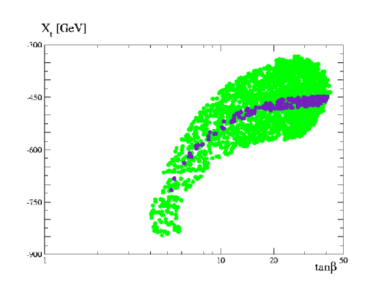
Figure 19: Constraints on $\tan\beta$ and $X_{t}\equiv A_{t}-\mu/\tan\beta$: indigo: one-$\sigma$ ($68\%$ C.L.) from a gaussian scan; green: same contour but for theoretical uncertainties $\Delta m_{h}=2$ GeV instead.

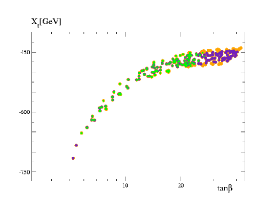
Figure 20: Constraints on $\tan\beta$ and $X_{t}\equiv A_{t}-\mu\tan\beta$: indigo: one-$\sigma$ ($68\%$ C.L.); orange: additional points at two-$\sigma$ ($95\%$ C.L.); green squares: remaining points (one-$\sigma$ level) when adding sbottom mass measurements.

We now apply the previous analysis to the reconstruction of some of the parameters related to the Higgs sector for the SPS1a test case with corresponding input mass accuracies. We perform again scan over parameters, taking into account the previous constraints on $m_{0}$ available from squark and slepton sector (and letting $X_{t}$ arbitrary), deriving joint constraints on $X_{t},\tan\beta$. The variation of other parameters which it implies (like e.g. the variation of $\mu$ from EWSB relations (VI)) is consistently taken into account. This is illustrated first in Fig. 19, where the range of points obtained from the prospected experimental accuracy: $\Delta m_{h}(\mbox{exp})\sim 0.25$ from Table 3 are shown. Also shown on the figure is the similar range now corresponding rather to the present theoretical uncertainties in the Higgs mass calculations (we take the latter as $\Delta m_{h}(\mbox{th})\sim 2$ GeVmh1-2loop ; adkps ). Note again that the density of points in the $\tan\beta,X_{t}$ plane has no precise statistical meaning: the larger “density” seen for rather large $\tan\beta$ is an artifact of the logarithmic scale. Also the one-$\sigma$ band which is thiner for low $\tan\beta$ and small $X_{t}$, is easily explained from the $m_{h}$ dependence on $\tan\beta$ and $X_{t}$: more precisely for fixed $\tan\beta$, $m_{h}(X_{t})$ reaches a maximum for a certain $X_{t}$ (see e.g. mh1-2loop ), and it is more difficult to match the approximate SPS1a value of $m_{h}$ for both small $\tan\beta$ and large (negative) $A_{0}$. The domain on $\tan\beta$ values obtained from this experimental Higgs mass measurement, at the one-$\sigma$ level, is thus approximately determined as:

$$5\raisebox{-3.69899pt}{~{}\shortstack{$<$ \\ [-0.07cm] $\sim$}}~{}\tan\beta\raisebox{-3.69899pt}{~{}\shortstack{$<$ \\ [-0.07cm] $\sim$}}~{}40\;.$$ (51)

These bounds are strongly correlated with $X_{t}$ values, as the figure shows. For $X_{t}$ one finds approximately:

$$-730\>\mbox{GeV}\raisebox{-3.69899pt}{~{}\shortstack{$<$ \\ [-0.07cm] $\sim$}}~{}X_{t}\raisebox{-3.69899pt}{~{}\shortstack{$<$ \\ [-0.07cm] $\sim$}}~{}-450\>\mbox{GeV}$$ (52)

Note also that all the points shown with relatively large $\tan\beta\sim 35-40$ are satisfying the previously mentioned theoretical constraint, with no tachyon $\tilde{\tau}_{1}$, since when departing from the SPS1a benchmark, larger values of $\tan\beta$ can be compensated by values of $A_{0}>-100$ GeV. (This is of course not taking into account any additional experimental constraints on $m_{h}$, $m_{\tilde{\tau}}$, etc which, as already emphasized, are omitted here since they are more model-dependent constraints.) The resulting limits on $X_{t}$ and $\tan\beta$ are of course sensitive to $m_{h}$ theoretical uncertainties as shown on the figures (though very little as concerns the $\tan\beta$ upper bound). In this case we obtain:

$$4\raisebox{-3.69899pt}{~{}\shortstack{$<$ \\ [-0.07cm] $\sim$}}~{}\tan\beta\raisebox{-3.69899pt}{~{}\shortstack{$<$ \\ [-0.07cm] $\sim$}}~{}40;\;\;\;-850\>\mbox{GeV}\raisebox{-3.69899pt}{~{}\shortstack{$<$ \\ [-0.07cm] $\sim$}}~{}X_{t}\raisebox{-3.69899pt}{~{}\shortstack{$<$ \\ [-0.07cm] $\sim$}}~{}-330\>\mbox{GeV}\;.$$ (53)

Table 7: Constraints on mSUGRA parameters $m_{0},m_{1/2},A_{0},\tan\beta$ obtained from a standard top-down $\chi^{2}$ fit of (first two generation) squark, sleptons, neutralino/gluino masses, plus the lightest Higgs mass, for different choices of MINUIT minimizations.

Data $\&$ fitted parameter	MIGRAD	MINOS	nominal
(+ model assumptions)	minimization ($68\%$C.L.)	minimization ($68\%$C.L.)	SPS1a value
$m_{\tilde{e}_{2}},m_{\tilde{u}_{1}}$, +
$m_{\tilde{N}_{1}},m_{\tilde{N}_{2}},m_{\tilde{g}}$ +$m_{h}$
(1-loop RGE + no $\tilde{q}$ R.C)	(convergent)	(problems)
$m^{q,l}_{0}$	99.96 $\pm 11.8$	99.9 ${}^{+11.5}_{-10}$	100
$m_{1/2}$	250 $\pm 4.9$	250 $\pm 4.9$	250
$A_{0}$	-100.5 $\pm 150.0$		-100
$\tan\beta(m_{Z})$	9.97 $\pm 4.3$	9.97 ${}^{+\mbox{no limits}}_{-4.3}$	10

However the contours shown in Fig. 19 did not take into account yet the additional constraints from the sbottom mass measurements which were obtained in previous section 5. This is now added in Fig. 20 (in green), where the one and two-$\sigma$ domains obtained from $m_{h}$ measurement are compared. One can see that at the two-$\sigma$ level the $X_{t}$ range increases slightly, for large $\tan\beta$, while $\tan\beta$ bounds are not much affected. On the other hand, the sbottom mass constraints put further upper limits on $\tan\beta\raisebox{-3.69899pt}{~{}\shortstack{$<$ \\ [-0.07cm] $\sim$}}~{}27-28$, in consistency with the previous analysis in section 5.

These results are also compared with a top-down MINUIT minimization in Table 7, using as input data $m_{h}$ in addition to the gluino cascade sparticle masses (but not yet using the sbottom masses at this stage). One observes that the MIGRAD symmetric error on $\tan\beta$ appears to be very good, but comparing with the contours in Figs. 19, 20 one can suspect that it is essentially influenced by the lowest limit on $\tan\beta$, and that the actual errors are particularly unsymmetrical due to the flat behaviour for large $\tan\beta$. This seems confirmed by the fact that the unsymmetrical MINOS positive error is not calculated by MINUIT. The lower $\tan\beta$ bound, on the other hand, is very consistent with our alternative finding in Eq. (51). This behaviour is well explained by the flattest dependence for large $\tan\beta$, as clearly illustrated by the plots in Figs. 19, 20. For completeness we also show in Fig. 21 the corresponding one- and two-$\sigma$ domains but in the $(\tan\beta,A_{0})$ plane, as well as the domain obtained once adding sbottom mass measurements. One can see that the sbottom mass bound have some impact on $A_{0}$ bounds, at least for large $-A_{0}$. These results may be compared with the $A_{0}$ limits obtained from the MINUIT fit in Table 7.

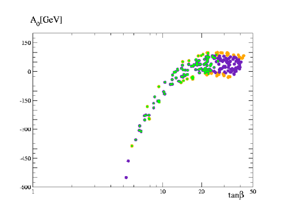
Figure 21: Contours from a Gaussian scan in the plane $(\tan\beta,A_{0})$: indigo: one-$\sigma$ ($68\%$ C.L.); orange: two-$\sigma$ ($95\%$ C.L.); green: remaining points (at one-$\sigma$) when adding sbottom mass measurements.

Thus the $m_{h}$ measurement alone gives a mild upper bound on $\tan\beta$ in the case where only some knowledge on $m_{A}(Q_{EWSB})$ is assumed (through sfermion-Higgs sector universality), but not on $X_{t}$. The improvement on $\tan\beta$ limits is mainly coming from adding the sbottom mass measurements. However this mild sensitivity, as well as the strong $\tan\beta-X_{t}$ correlation, is essentially determined by the variation of $A_{0}$ which is assumed unknown at this stage. The uncertainties on $\mu$ (that are reasonable in this constrained MSSM case) have little influence (except perhaps for very small $\tan\beta$), since it is suppressed as $\mu/\tan\beta$ within $X_{t}$. We shall see in the summarizing section VI.4 that overall, the bounds are a bit tighter once combining all available informations, except those for $A_{0}$ which depend quite much on the level of approximation used in RGE and radiative corrections. If an additional independent information on $A_{0}$ would be available (e.g. if the stop masses could be measured) the constraints in the $\tan\beta,X_{t}$ plane could be evidently improved. Better constraints on $\tan\beta$ are also prospectedLHCstudy clearly if some of the heavy Higgses $A,H,H^{\pm}$ could be measured, that we do not assume in our ‘minimal’ set of input mass measurements and within the SPS1a benchmark case. (It would be rather straightforward, however, to extend our above analysis in case such additional information would be available.)

We finally mention that our results are not drastically changing once using the more complete two-loop level radiative corrections for $m_{h}$ (assuming in such case universality/mSUGRA relations to calculate all higher order corrections), except for the bounds on $A_{0}$ that are substantially worsened in this case, as will be confirmed by further MINUIT fit results summarized in section VI.4. This comes from an observed flattest dependence of $m_{h}(A_{0})$ for large $-A_{0}$ at the two-loop level, in the range considered for the other relevant parameters. As far as we can see, this may be explained by the fact that within the two-loop level radiative corrections to $m_{h}$mh1-2loop ; bdsz , there is somewhat much room for possible cancellations of the $A_{0}$ dependence entering in higher orders, most notably in all squark and stau contributions both at the one- and two-loop level. This is another example of the caution needed to interpret results when performing minimization constraints using different level of theoretical approximations.

VI.4 Combining all information and comparison with standard fits

Table 8: Combined best constraints from all gluino cascade decay sparticles and lightest Higgs mass measurements for the bottom-up approach in different MSSM scenarios. (NB a star in superscript indicates discrete ambiguities in the reconstruction in the non-universal MSSM case, as discussed e.g. in sub-sec. 3.1 and Appendix A).

Model or assumptions	Parameter	Constraint (GeV)	nominal SPS1a value
			(from SuSpect 2.41)
general MSSM	$M_{1}(Q_{EWSB})^{\star}$	$\sim$95–115	101.5
” ”	$M_{2}(Q_{EWSB})^{\star}$	$\sim$175–225	191.6
” ”	$M_{3}(Q_{EWSB})$	$\sim$580–595	586.6
” ”	$(\frac{3}{8}m^{2}_{u_{L}}+\frac{m^{2}_{e_{R}}}{4})^{1/2}(Q_{GUT})$	$\sim$68–89	$(\frac{5}{8})^{1/2}100\sim 79$
” ”	$m_{Q3_{L}}(Q_{EWSB})^{\star}$	$\sim$488–518	497
” ”	$m_{b_{R}}(Q_{EWSB})^{\star}$	$\sim$510–540	522
” ”	$\mu(Q_{EWSB})^{\star}$	$\sim$280–750	357
” ”	$\tan\beta(Q_{EWSB})$	$\sim$1–36 (th. bounds)	9.74
+ $m_{\tilde{N}_{4}}$	$\mu(Q_{EWSB})^{\star}$	$\sim$350–372	357
” ”	$\tan\beta(Q_{EWSB})$	$\sim$2.7–36 (th. bounds)	9.74
$\tilde{q},\tilde{l}$-universality	$m^{q,l}_{0}(Q_{GUT})$	$\sim$90–112	100
” ”	$m_{Q3_{L}}(Q_{EWSB})$	$\sim$490–506	497
” ”	$m_{b_{R}}(Q_{EWSB})$	$\sim$513–530	522
$M_{i},i=1,..3$-universality	$M_{i}(Q_{GUT})$	$\sim$ 245–255	250
$\tilde{b}_{1},\tilde{b}_{2}$ +universality	$\tan\beta(Q_{EWSB})$	$\sim$3–28	100
mSUGRA	$m_{0}$	$\sim$90-112	100
	$m_{1/2}$	$\sim$245–255	250
	$-X_{t}$	$\sim$450–730	530
	$-A_{0}$	$\sim$ -100-350	100
	$\tan\beta(m_{Z})$	$\sim$ 5.5–28	10

We finally summarize and combine all previous constraints from the different sectors, both in general MSSM or with universality relations, in Table 8. By “combined best constraints” we simply mean to evaluate the joint limits by crudely superposing the constraints obtained in the three different sectors of gaugino/Higgsino, squarks/sleptons and Higgs, which eventually results in slight improvements on some parameter limits. We did not attempt to perform a more elaborated statistical combination of the three sector constraints within our present approach. However, these results are compared with those obtained from a top-down $\chi^{2}$ fit of basic mSUGRA parameters to the same mass measurements in Table 9. As one can see, the results are overall qualitatively consistent, except perhaps for the $A_{0}$ limits. The fact that $A_{0}$ bounds (and to some extent $\tan\beta$ bounds as well) are worsen when fitting parameters in mSUGRA at the full two-loop level instead of one-loop, was explained previously due to the possible cancellations of the $A_{0}$ dependence in higher order $m_{h}$ contributions. Note that for $\tan\beta$, the MIGRAD symmetric minimization error found here appears very optimistic as compared to the upper bound derived from the bottom-up reconstruction, $\tan\beta\raisebox{-3.69899pt}{~{}\shortstack{$<$ \\ [-0.07cm] $\sim$}}~{}28$. As already mentioned above it is possibly much influenced by the lower bound that results from the combination with the Higgs sector measurements. The MINOS upper bound is however more consistent with the bottom-up result.

Table 9: Combined constraints on mSUGRA basic parameters from a standard top-down $\chi^{2}$ fit with MINUIT of all gluino cascade decay sparticle masses plus $m_{h}$ measurements.

Model and assumptions	Parameter	$68\%$ C.L. limits (GeV)	SPS1a value
mSUGRA	$m_{0}$	99.96 $\pm$ 11.2	100
2-loop RGE + full $\tilde{q}$ R.C. + 2-loop $m_{h}$		(99.95 $\pm$ 11.7)
(1-loop RGE+ no $\tilde{q}$ R.C. +simple $m_{h}$ R.C.)	$m_{1/2}$	250.0 $\pm$ 3.7	250
		(249.5 $\pm$ 4.7)
	$A_{0}$	-104.2 $\pm 379$	-100
		(-100.6 $\pm 136$)
	$\tan\beta(m_{Z})$	9.9 ${}^{+9.4}_{-4.7}$	10
		(9.96 $\pm 4.11$)

VII Conclusion

We have examined some specific bottom-up reconstruction strategies at the LHC, both for general and universality-constrained MSSM parameters, starting from a plausible set of incomplete measurements of a few MSSM sparticles. Using sparticle mass measurements mainly from cascade decays of gluino and squarks, and the lightest Higgs boson mass, we have constructed different algorithms, based on rather simple semi-analytical inverse relations between the MSSM basic parameters and mass spectrum, incorporating radiative corrections, when known, at a realistic level. We have determined constraints on the relevant basic MSSM parameters from the expected mass accuracies, under different theoretical assumptions on the degree of universality of some of the parameters. We have also exhibited analytically the possible discrete ambiguities in the reconstruction of some of the basic parameters, when using only mass input in a general unconstrained MSSM without extra knowledge or assumptions on the relative hierarchy of the relevant parameters. This is the case in particular for the gaugino/Higgsino sector parameters. These constraints have been also compared at different stages in a sector-by-sector analysis, with those obtained from more conventional top-down approaches of fits to data with minimization procedures. The results are overall consistent, which is an a posteriori check that our rather naive semi-analytic approach, with many approximations, does essentially capture the sensitivity on parameters.

Regarding the SPS1a reconstruction example studied here, more quantitatively we have shown that a rather limited data set, consisting of merely the measurement of sparticle masses involved in gluino cascade decay to a few percent accuracy, may still provide reasonably good constraints on some of the relevant MSSM parameters. This is in particular the case for the gaugino mass parameters and the squark and slepton soft mass terms, even for an unconstrained MSSM without universality assumptions. If a precise measurement of the lightest Higgs mass is available, additional constraints (though moderate) on $\tan\beta,X_{t}\equiv A_{t}-\mu/\tan\beta$ are obtained, but only if Higgs-sfermion mass term universality is assumed. Interesting constraints for a non-universal MSSM are however more challenging to obtain in general for the Higgs sector parameters (as well as for $\tan\beta$), unless more precise measurements would be available (or data from another sector, like heavy Higgses and/or scalar top masses typically), as is also known from other analysisLHCstudy . We stress again that considering only the gluino/squark cascade (plus the lightest Higgs) sparticle identification in our analysis is not motivated by a strong prejudice against other potential SUSY-discovery processes at the LHC. Indeed the cascade in Eq. (1) may be considered already quite specific from a general MSSM viewpoint, but it gives us a well-defined and rather minimal input set for testing our approach, and comparing it with other analyses for the very much studied SPS1a benchmark. Even if our results are probably not very new to the experts, they illustrate that a step-by-step semi-analytic approach can help to exhibit better the sensitivity of basic MSSM parameters with respect to given sparticle mass or other data, which may be more difficult to grasp from global top-down fits. In many cases, the non-linear and non-symmetric behaviour of error propagations is exhibited by our analytic bottom-up approach in a more explicit way (as illustrated typically for $\tan\beta$, comparing Tables 8 and 9), and similarly for the possible discrete ambiguities e.g. in the gaugino/Higgsino sector. As compared to other recent analysis of MSSM constraints at LHC (e.g. LHCstudy ; dzerwas ; mssmbayes ; ben_bayes ), our results are difficult to compare quantitatively in very detail, since the data used are often different (with generally more input sparticle masses assumed in most other analysis). We find however a rough consistency on the expected sensitivity of the basic MSSM parameters, as discussed above.

The relatively simple algorithms described here are rather flexible, and may be easily interfaced with more elaborated simulation tools, that would allow in particular a more realistic statistical treatment of the different sources of experimental and theoretical uncertainties. Moreover, some of our analytical relations may be used at least as “Bayesian priors” guideline to other analysis, in a way complementary to the Markov chain techniques. We plan indeed a more refined statistical analysis in the futureprepa , by possibly combining our approach with Bayesian and Markov chain techniques of ref. mssmbayes ; ben_bayes ; dzerwas .

Our approach may thus provide a useful complementarity to more elaborated simulations, as well as possible cross-checks. Moreover it is not at all restricted to the LHC phenomenology: some of the algorithms described here, for instance in the neutralino and squark/slepton sectors, may be readily used for ILC data upon straightforward changes in sparticle mass accuracies. However, a similar approach for the ILC, following e.g. the studies made in refs. zerwasetal ; otherinv , deserves specific analysis beyond the scope of the present paper, due to the different sparticle spectrum expected to be reached at the ILC, which will imply slightly different inversion algorithms.

Acknowledgements
This work is partially supported by ANR contract “PHYS@COL$\&$COS” and GDR 2305 “Supersymétrie”. We are grateful to Gilbert Moultaka for stimulating conversations at a preliminary stage of this work. We also thank Dirk Zerwas, Ulrich Ellwanger and Sabine Kraml for interesting comments or discussions.

Appendix A Solving the gaugino/Higgsino parameters for different input

In this appendix, we give for completeness explicit analytic solutions relating neutralino masses and gaugino/higgsino parameters, depending on different input and output choice and depending on general MSSM or more constrained universality assumptions, relevant to sections 3.1-3.4.

A.1 Two neutralino mass input

From Eqs. (10), (11), one can solve $M_{1},M_{2}$ for input masses $m_{\tilde{N}_{1}},m_{\tilde{N}_{2}}$, plus $\mu$, $\tan\beta$ input: after expressing $M_{1}$ e.g. from Eq. (10) (see also inv1 ):

$$M_{1}=-\frac{P_{12}\left[\mu^{2}+m^{2}_{Z}+P_{12}+(M_{2}-S_{12})S_{12}\right]+M_{2}\,\mu\,m^{2}_{Z}s^{2}_{W}\sin 2\beta}{S_{12}P_{12}-M_{2}(\mu^{2}+P_{12})+c^{2}_{W}m^{2}_{Z}\mu\sin 2\beta}\;,$$ (54)

(with $S_{12}\equiv m_{\tilde{N}_{1}}+m_{\tilde{N}_{2}}$, $P_{12}\equiv m_{\tilde{N}_{1}}m_{\tilde{N}_{2}}$), $M_{2}$ is given by a standard second order equation with solution:

$$M_{2}=\frac{-b_{1}\pm\sqrt{b^{2}_{1}-4a_{1}c_{1}}}{2a_{1}}$$ (55)

where $+\sqrt{\dots}$ corresponds to $M_{1}<M_{2}$ and $-\sqrt{\cdots}$ to $M_{2}<M_{1}$ respectively, and

$$a_{1} = P_{12}\left[\mu^{4}+P_{12}(P_{12}+m^{2}_{Z}s^{2}_{W})+\mu^{2}(2P_{12}-S_{12}^{2}+m^{2}_{Z}s^{2}_{W})+\mu\,m^{2}_{Z}s^{2}_{W}\sin 2\beta\,S_{12}\right]$$

$$b_{1} = P_{12}\left[S_{12}(-\mu^{4}+\mu^{2}(-m^{2}_{Z}-2P_{12}+S_{12}^{2})-P_{12}(P_{12}+m^{2}_{Z}(s^{2}_{W}-c^{2}_{W}))\right.$$

$$\left.-\mu\,m^{2}_{Z}(P_{12}+(S_{12}^{2}-P_{12})(s^{2}_{W}-c^{2}_{W})+2\mu^{2}c^{2}_{W})\sin 2\beta\right]$$

$$c_{1} = P_{12}(P_{12}(\mu^{2}+m^{2}_{Z}+P_{12})(\mu^{2}+c^{2}_{W}m^{2}_{Z}+P_{12})-(\mu^{2}+c^{2}_{W}m^{2}_{Z})P_{12}S_{12}^{2}$$ (56)

$$+\mu\,m^{2}_{Z}\,\sin 2\beta(S_{12}(P_{12}+c^{2}_{W}(\mu^{2}+m^{2}_{Z}+2P_{12}-S_{12}^{2}))+c^{2}_{W}m^{2}_{Z}\,\mu\,\sin 2\beta))\;.$$

The occurrence of two $M_{2}$ solutions in Eq. (55) is due to the structure of Eqs. (10), (11), but this ambiguity cannot be resolved from the sole knowledge of two neutralino mass input, since all the available relations from Eqs. (9) are completely symmetrical under $m_{\tilde{N}_{1}}\leftrightarrow m_{\tilde{N}_{2}}$ permutations. Typically in the simple limit of neglecting all $D$-terms i.e. $m_{Z}\to 0$ in the neutralino mass matrix Eq. (8), the four neutralino mass eigenvalues are trivially given as

$$m_{\tilde{N}_{i}}(i=1,..,4)=M_{1},M_{2},|\mu|,|\mu|\;.$$ (57)

with all possible permutations i.e no ordering implied. The exact mass eigenvalues with $m_{Z}\neq 0$ are no longer invariant under e.g. $M_{1}\leftrightarrow M_{2}$ permutations, but concerning the inverted relations, even if all physical masses were known and thus ordered according to e.g $m_{\tilde{N}_{1}}<\cdots<m_{\tilde{N}_{4}}$, there is no way to determine from the sole knowledge of a given mass $m_{\tilde{N}_{i}}$ if it corresponds to a Bino, Wino or Higgsino. This needs information on diagonalization matrix elements, that can be partly accessed if measuring the couplings of neutralinos to other particles. (However, for known $\mu$ input, measuring a third neutralino mass could in principle solve the $M_{1},M_{2}$ ambiguity, since the two different solutions gives different $m_{\tilde{N}_{3}},m_{\tilde{N}_{4}}$ (which are most simply obtained by solving Eq. (13) as a second order equation for e.g. $m_{\tilde{N}_{4}}$). But in practice this needs an accurate knowledge of both $\mu$ and the three neutralino masses).

In Fig. 22 the two $M_{1},M_{2}$ solutions are illustrated as functions of $\mu$ (see respectively $M_{2}(1,2)$ and $M_{1}(1,2)$), with the two neutralino mass input and $\tan\beta$ fixed to SPS1a values for reference. Note that in Eq. (55) there can be values of $\mu$, $\tan\beta$ for which $a_{1}\to 0$: for example for SPS1a values of $\tan\beta$, $a_{1}(\mu,\tan\beta)$ has four zeros for real values of $\mu$: $\mu\sim-165,-110,118,157$ GeV. However these poles with respect to $\mu$ are artifacts since for $a_{1}=0$ strictly, the (unique) solution reduces to $M_{2}=-c_{1}/b_{1}$ (moreover the possible zeros of $b_{1}(\mu)$ do not coincide with those of $a_{1}(\mu)$). Nevertheless sufficiently close to these $\mu$ “pole” values, one of the two $M_{2}$ solutions can become arbitrarily large, as can be seen on Fig. 22 . More physically, this means that such large values of $M_{2}$, with their corresponding $\mu$ pole values, are still consistent with the same neutralino masses $m_{\tilde{N}_{1}},m_{\tilde{N}_{2}}$.

As such, Eq. (55) is not very illuminating: it may be useful to expand to first order in the $D$-term, i.e. to ${\cal O}(m^{2}_{Z})$, which gives a very simple expression:

$$M_{2}=m_{\tilde{N}_{2}}+c^{2}_{W}m^{2}_{Z}\frac{(m_{\tilde{N}_{2}}+\mu\sin 2\beta)}{\mu^{2}-m^{2}_{\tilde{N}_{2}}}$$ (58)

for the case $M_{1}<M_{2}$ (and the same expression with $m_{\tilde{N}_{2}}\to m_{\tilde{N}_{1}}$ for the case $M_{2}<M_{1}$). (For $M_{1}$ one better keeps the exact and relatively simple expression Eq. (54)). Here the pole at $\mu=m_{\tilde{N}_{i}}$ in Eq. (58) is clearly an artifact of first order in $m^{2}_{Z}$ expansion, and simply reflects that this approximation is not valid for $\mu\sim m_{\tilde{N}_{i}}$. Eq. (58) is certainly a good approximation for $\mu\gg m_{\tilde{N}_{1}},m_{\tilde{N}_{2}}$ and $m_{\tilde{N}_{i}}\gg m_{Z}$. Moreover it can still be a rather good approximation even for moderate $\mu$ and neutralino mass values. For instance for SPS1a values in Table 2, and neglecting self-energy radiative corrections to neutralino masses one has $\mu\sim 357$ GeV, $m_{\tilde{N}_{2}}\sim 176.2$ GeV and $M^{exact}_{2}(SPS1a)\sim 191.6$ while $M^{approx}_{2}(SPS1a)\sim 192.6$ which is only $.5\%$ difference, i.e. less than the magnitude of radiative corrections to neutralino masses, which are about $\sim 4$ GeV for $m_{\tilde{N}_{2}}$. We have used however the exact expressions (55) throughout our analysis in section 3.

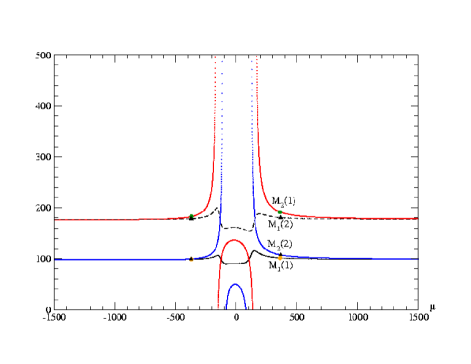
Figure 22: The two $M_{1},M_{2}$ solutions (respectively $M_{2}(1,2)$ and $M_{1}(1,2)$) from Eqs. (54), (55) for two neutralino mass $m_{\tilde{N}_{1}}$, $m_{\tilde{N}_{2}}$ input, as functions of $\mu$. The dots and triangles corresponds to the solutions once a third neutralino mass $m_{\tilde{N}_{4}}$) input is used, completely determining $|\mu|$ (for fixed $\tan\beta$). The neutralino mass input values and $\tan\beta$ are fixed to their SPS1a values for illustration.

A.2 Three neutralino mass input: general case

Knowing three neutralino masses allow to use one more equation from (9) to solve e.g. for $M_{1}$, $M_{2}$ and $\mu$ in terms of the three neutralino masses and $\tan\beta$ input values. (Alternatively, we could also solve this system to determine rather $\tan\beta$ for fixed $\mu$, but since it only depends on $\sin 2\beta$, any $\tan\beta$ dependence drops out for large $\tan\beta$. Thus we can anticipate without calculations that there can be no interesting $\tan\beta$ upper bounds, irrespectively of the number of neutralino masses measured, given their expected LHC accuracies). The extra relation to determine $\mu^{2}$ is Eq. (13) obtained from the trace and second invariant in Eq. (9). Note however that the sign of $\mu$ is still not determined. Combining Eq. (13) with Eqs. (10), (11) gives a high (sixth) order polynomial equation in $\mu$ (or equivalently in $M_{1}$ or $M_{2}$) which cannot be solved fully analytically. It is however easy to solve iteratively using e.g. Eq. (13) on the solutions (55), (54) (upon having chosen a definite order for the relative values of $M_{1}$ and $M_{2}$). This iterative solution converges very quickly. The solutions for $M_{1}$, $M_{2}$ and $\mu$ obtained for $\tan\beta$ input fixed to SPS1a value are illustrated by the different dots and triangles in Fig. 22.

Alternatively it is useful to consider, as in the case of two neutralino masses above, approximate solutions obtained by expanding to first order in $m^{2}_{Z}$. This gives very simple expressions:

$$M_{1} = m_{\tilde{N}_{1}}+s^{2}_{W}m^{2}_{Z}\frac{(m_{\tilde{N}_{1}}+m_{\tilde{N}_{3}}\sin 2\beta)}{m^{2}_{\tilde{N}_{3}}-m^{2}_{\tilde{N}_{1}}}$$

$$M_{2} = m_{\tilde{N}_{2}}+c^{2}_{W}m^{2}_{Z}\frac{(m_{\tilde{N}_{2}}+m_{\tilde{N}_{3}}\sin 2\beta)}{m^{2}_{\tilde{N}_{3}}-m^{2}_{\tilde{N}_{2}}}$$

$$|\mu| = m_{\tilde{N}_{3}}-\frac{m^{2}_{Z}}{2}(1+\sin 2\beta)\>\frac{[m_{\tilde{N}_{3}}-m_{\tilde{N}_{2}}+c^{2}_{W}(m_{\tilde{N}_{2}}-m_{\tilde{N}_{1}})]}{(m_{\tilde{N}_{3}}-m_{\tilde{N}_{1}})(m_{\tilde{N}_{3}}-m_{\tilde{N}_{2}})}$$ (59)

corresponding to the first case $M_{1}<M_{2}$ (i.e. a Bino LSP), and similar expressions with $m_{\tilde{N}_{1}}\leftrightarrow m_{\tilde{N}_{2}}$ for the case $M_{2}<M_{1}$. Actually, considering three neutralino mass input and $M_{1},M_{2},\mu$ output adds more discrete ambiguities than in the two neutralino mass case: accordingly in a most general MSSM, without further knowledge on e.g. neutralino couplings, or further theoretical assumptions, one should in principle consider all possible ordering among $M_{1}$, $M_{2}$, $\mu$ values, i.e. six possible cases (where the LSP mass $m_{\tilde{N}_{1}}$ can be either Bino, Wino or Higgsino). It is straightforward to derive such other solutions by appropriate permutations of the three $m_{\tilde{N}_{i}}$, within Eqs. (59). For all cases Eqs. (59) are very good approximations, at least as far as $m_{\tilde{N}_{i}}$ are not small compared to $m_{Z}$, e.g. for the SPS1a case typically the differences with exact results is of order or below the percent level.

A.3 gaugino mass universality: two or three neutralino mass input

Assuming gaugino mass universality one can solve again Eqs. (10), (11) but changing input/output: now the EWSB scale values of $M_{1}$ and $M_{2}$ are given from $M_{3}$ by Eq. (12), so that one can determine $|\mu|$ and $\tan\beta$ assuming two neutralino mass input from a linear system, which gives

$$\mu^{2}=-\frac{b_{2}}{a_{2}}$$ (60)

with

$$a_{2} = P_{12}\,(M_{1}+M_{2}-S_{12}+\frac{P_{12}-M_{1}M_{2}}{M_{12}}\,)$$

$$b_{2} = P_{12}\,\left[P_{12}\,(M_{1}+M_{2}-S_{12})+S_{12}\left((M_{1}-m_{\tilde{N}_{1}})(M_{2}-m_{\tilde{N}_{1}})-(M_{1}+M_{2}-m_{\tilde{N}_{1}})m_{\tilde{N}_{2}}\right.\right.$$ (61)

$$\left.\left.+m^{2}_{\tilde{N}_{2}}-m^{2}_{Z}\right)+m^{2}_{Z}\left(M_{12}+\frac{P_{12}\left(P_{12}+(M_{1}-S_{12})(S_{12}-M_{2})+m^{2}_{Z}\right)}{m^{2}_{Z}M_{12}}\right)\right]$$

and

$$\sin 2\beta = -\frac{\left[P^{2}_{12}-M_{1}M_{2}\mu^{2}+P_{12}\,((M_{1}+M_{2})S_{12}-M_{1}M_{2}-S^{2}_{12}+\mu^{2}+m^{2}_{Z})\right]}{\mu\,m^{2}_{Z}M_{12}}$$ (62)

with $M_{12}\equiv c^{2}_{W}M_{1}+s^{2}_{W}M_{2}$ and other notations as in Eqs. (54)-(56). Note that we assume $\mu$ to be real. The case of three neutralino mass input is treated by combining Eq. (13)-Eq. (62).

Appendix B Bottom-up renormalization group evolution in SuSpect code

In this section we illustrate in some details an important ingredient of our bottom-up reconstruction procedure which is the renormalization group evolution (RGE)rge ; RGE2 of MSSM parameters from low to high energy. We take this opportunity to present the results from an available option of the SuSpect code, illustrating some properties of this bottom-up RG evolution which are quite general and independent of the present analysis and LHC cascade decay phenomenology. (This option has recently been adapted to the more suitable “Les Houches accord” input file conventionsslha .)
The fact that the RGE for the MSSM parameters are “invertible”, i.e can be evolved from high to low scale and backward, is a rather obvious feature of any such coupled differential equations. However, what makes it less straightforward in the standard approach to MSSM calculation with RGE, is that there are actually three (at least) different energy scales in the game, with corresponding boundary conditions:

• the high (generally GUT) scale, at which one defines e.g. the mSUGRA parameters with eventually some universality relations;

• the (low) electroweak symmetry breaking scale, at which the soft breaking and other relevant MSSM parameters are evolved to in a standard top-down evolution;

• finally the scale $m_{Z}$, or eventually some other low energy scale, which enter as other boundary conditions e.g; via the precise measurements of the gauge couplings.

The interplay between these different scales in MSSM spectrum calculation codes (such as SuSpect suspect and similar codesisasugra ; softsusy ; spheno ) needs, among other things, iterative algorithms for the evolution between the three different scale, with a consistent implementation of any possibly known radiative corrections to the parameters (gauge couplings, top, bottom masses, etc) entering as boundary conditions to the RG evolution. (We refer to the SuSpect manual suspect for details on such RGE algorithms.)

Such a bottom-up evolution option has been available in a beta-version for some time in SuSpect but was not publicly available nor illustrated until now. In Table 10 we illustrate for the SPS1a benchmark point this bottom-up RG evolution of all parameters. We show in particular some important features on the error propagation in such a procedure, and which parameters are more sensitive to this dispersion. The input parameters (in the second column) were obtained in a first stage from a standard (top-down) run from the mSUGRA SPS1a input parameters in Eq. (2) (with $m_{top}=175$ GeV). The third column gives the corresponding output values resulting from a RG evolution up to a GUT scale from a bottom-up SuSpect run under the most general MSSM assumptions, i.e. without any a priori on possible universality relations at the GUT scale. One can already notice from this that the agreement with the original mSUGRA parameter values is excellent: the discrepancies are of order ${\cal O}(10^{-3})$ that are in fact consistent with the accuracy chosen (i.e. the intrinsic error of the numerical evolution of the RGE as performed with a Runge-Kutta algorithm, as well as the intrinsic error due to necessary iterative proceduressuspect ). We point out however that the results shown here correspond to the choice of $m_{H_{u}}$, $m_{H_{d}}$ input, while the correspond results for $m_{A}$, $\mu$ input choice are a little bit worse for $m_{H_{u}}(Q_{GUT})$ and $m_{H_{d}}(Q_{GUT})$, which is attributed to a certain precision loss in our algorithm when passing from one to the other input set, that involves calculations and iterations including two-loop radiative corrections. (This is in particular due to the well-known $Tr[YM^{2}]$ terms present in the RGErge ; RGE2 , which involve a combination of soft scalar terms, including $m^{2}_{H_{u}}$ and $m^{2}_{H_{d}}$: this combination vanishes by definition in mSUGRA, and remains zero at all scales in a top-down RG evolution. However, when using bottom-up RGE the approximate $m^{2}_{H_{u}},m^{2}_{H_{d}}$ values as obtained from $m_{A},\mu$ from EWSB conditions Eqs. (VI) does not satisfy $Tr[YM^{2}]=0$ exactly, and this induces a not completely negligible departure when evolving from low to GUT scales.)

Next, the fourth and subsequent columns give the deviations in the output parameter values corresponding to $\pm 1\%$ deviations of some relevant parameters input values: $M_{3}$, $m_{H_{u}}$, $m_{Q3_{L}}$, that we chose on purpose as they give the most important sensitivity to other parameters deviations. One can see that the deviations induced in other parameters remain generally reasonable, at the percent level, notably for the gaugino masses, and most of the squark and sleptons (except for the one sfermion mass which is varied in each case). In contrast, the deviations induced on the scalar mass $m_{H_{u}}$ can be huge, even for a moderate percent deviation, i.e. there is a large amplification or dispersion of error. This is of course explained from the detailed RGE dependence of $m_{H_{u}}$ on other soft terms, resulting in a very strong sensitivity on certain other parameters. The same is true to some extent for $m_{t_{R}}$. The strong sensitivity of $m_{H_{u}}$ e.g. on the top mass value and other parameters through its RGE is a well-know feature, but more precisely our illustration here indicate that it will be very difficult to have a precise determination of $m_{H_{u}}$ at a high GUT scale, even in the very optimistic case where all other MSSM parameters would be know quite precisely. Consequently it will be very difficult to check for eventual universality of the soft scalar mass terms with the squark and slepton soft terms. One can however turn this argument the other way round, and deduce from this illustration that, while $m_{H_{u}}$ plays a crucial role in the (radiative) electroweak symmetry breaking, the sparticle masses at low scale determining most of the collider phenomenology are not very much dependent on its precise value at GUT scale. (This is somewhat similar here to the “focus point” properties observed for large $m_{0}$ values in other mSUGRA parameter choices). More generally, many features as those illustrated in Table 10 may be important to keep in mind for any realistic bottom-up procedure. The above bottom-up RGE procedure had been used in several stages of our analysis, as indicated in the main text.

Table 10: Bottom-up RG evolution of SPS1a parameters from SuSpect 2.41 with illustration of error propagations. Input parameters (2nd column) were obtained from a standard (top-down) SuSpect run from SPS1a input parameters in Eq. (2) (with $m_{top}=175$ GeV). The third column gives corresponding output values once evolved back to a GUT scale from a bottom-up SuSpect run with general MSSM option. Fourth and subsequent columns give deviations in the output parameter values corresponding to $\pm 1\%$ deviations of some relevant parameters input values as indicated. (Variation range is given explicitly when non-symmetrical)

par.	input(GeV)	GUT output	$\Delta M_{3}=\mp 1\%$	$\Delta m_{H_{u}}=\mp 1\%$	$\Delta m_{Q3_{L}}=\mp 1\%$
$Q_{EWSB}$	465.5	$\simeq 2.47\>10^{16}$	0.1 $\%$	0.1$\%$	$0.1\%$
$M_{1}$	101.5	250.004	negl.	negl.	negl.
$M_{2}$	191.6	249.998	” ”	” ”	” ”
$M_{3}$	586.6	249.999	$\pm 2.2$	” ”	” ”
$m^{2}_{H_{d}}$	$(179.9)^{2}$	$(100.004)^{2}$	$(100.6)^{2}$–	$(100.7)^{2}$–	$(101.2)^{2}$–
			$(99.4)^{2}$	$(99.2)^{2}$	$(98.7)^{2}$
$m^{2}_{H_{u}}$	$-(358.1)^{2}$	$(100.017)^{2}$	$(132.6)^{2}$–	$(64.9)^{2}$–	$(63.7)^{2}$–
			$(48.4)^{2}$	$(124.4)^{2}$	$(126.4)^{2}$
($m^{pole}_{A}$)	398.8
($\mu$)	356.9	353
$m_{e_{L}}$	195.5	100.004	100.2–99.8	100.8–99.2	101.5–98.5
$m_{\tau_{L}}$	194.7	100.004	100.2–99.8	100.8–99.2	101.5–98.5
$m_{e_{R}}$	136	99.998	100–99.9	98.4–101.6	96.8–103.1
$m_{\tau_{R}}$	133.5	99.998	100–99.9	98.4–101.6	96.8–103.1
$m_{Q1_{L}}$	545.8	100.001	121–72	99.7–100.3	99.1–100.8
$m_{Q3_{L}}$	497	100.005	131–52	94.6–104.6	55.2–130.4
$m_{u_{R}}$	527.8	99.997	121–72	101–99	101.8–98.1
$m_{t_{R}}$	421.5	100.006	140–14	90.6–107.5	81.9–115.3
$m_{d_{R}}$	525.7	99.997	121–72	99.4–100.6	98.7–101.3
$m_{b_{R}}$	522.4	99.997	122–72	99.4–100.6	98.5–101.5
$-A_{t}$	494.5	100.009	$111--89$	” ”	” ”
$-A_{b}$	795.2	100.002	$106--94$	” ”	” ”
$-A_{\tau}$	251.7	100.002	$100--99.9$	” ”	” ”
$-A_{u}$	677.3	100.005	$108--92$	negl.	negl.
$-A_{d}$	859.4	100.001	$105--95$	” ”	” ”
$-A_{e}$	253.4	100.002	$100--99.9$	” ”	” ”
$\tan\beta$	9.74

References

- (1) For reviews on the MSSM, see: H. P. Nilles, Phys. Rept. 110, 1 (1984); R. Barbieri, Riv. Nuovo Cim. 11N4, 1 (1988); R. Arnowitt and Pran Nath, Report CTP-TAMU-52-93; M. Drees and S.P. Martin, hep-ph/9504324; J. Bagger, Lectures at TASI-95, hep-ph/9604232; S.P. Martin, hep-ph/9709356; S. Dawson, hep-ph/9712464.
- (2) B.C. Allanach, C.G. Lester, M.A. Parker and B.R. Webber, JHEP 0009 (2000) 004.
- (3) B.K. Gjelsten, D.J. Miller and P. Osland, JHEP 0412 (2004) 003 (hep-ph/0410303).
- (4) B.K. Gjelsten, D.J. Miller and P. Osland, JHEP 0506 (2005) 015 (hep-ph/0501033).
- (5) G. Weiglein et al, Phys. Rept. 426 (2006) 47 (hep-ph/0410364).
- (6) J.A. Aguilar-Saavedra et al, Eur. Phys. J. C46 (2006)43 (hep-ph/0511344).
- (7) There is a very large amount of literature on this subject. For a very non-exhaustive list of relatively recent works, see e.g.: H. Baer, C. Balazs, A. Belyaev, J.K. Mizukoshi, X. Tata and Y. Wang, JHEP 0207, 050 (2002), hep–ph/0205325; H. Baer and C. Balazs, JCAP 0305, 006 (2003), hep-ph/0303114; H. Baer, C. Balazs, A. Belyaev, T. Krupovnickas and X. Tata, JHEP 0306, 054 (2003) [arXiv:hep-ph/0304303]; U. Chattopadhyay, A. Corsetti and P. Nath, Phys. Rev. D68, 035005 (2003) hep–ph/0303201; J.R. Ellis, K.A. Olive, Y. Santoso and V.C. Spanos, Phys. Lett. B565, 176 (2003), hep-ph/0303043; M. Battaglia, A. De Roeck, J.R. Ellis, F. Gianotti, K.A. Olive and L. Pape, Eur. Phys. J. C33, 273 (2004), hep–ph/0306219; M.E. Gomez, T. Ibrahim, P. Nath and S. Skadhauge, Phys. Rev. D70, 035014 (2004); A. Djouadi, M. Drees and J. L. Kneur, JHEP 0603, 033 (2006) [arXiv:hep-ph/0602001]; U. Chattopadhyay, D. Das, A. Datta and S. Poddar; Phys. Rev. D 76, 055008 (2007) [arXiv:0705.0921 [hep-ph]].
- (8) J.R. Ellis, K.A. Olive, Y. Santoso and V. Spanos, Phys.Rev. D 69 (2004) 095004 [arXiv:hep-ph/0310356]; J.R. Ellis, S. Heinemeyer, K.A. Olive and G. Weiglein, JHEP 0502 (2005) 013 [arXiv:hep-ph/0411216]; E.A. Baltz and P. Gondolo, JHEP 0410 (2004) 052 [arXiv:hep-ph/0407039]; B.C. Allanach and C.G. Lester, Phys. Rev. D73 (2006) 015013 [arXiv:hep-ph/0507283]; B.C. Allanach, Phys.Lett. B635 (2006) 123 [arXiv:hep-ph/0601089]; R. Ruiz de Austri, R. Trotta and L. Roszkowski, JHEP 0605 (2006) 002 [arXiv:hep-ph/0602028]; E. Baltz, M. Battaglia, M. Peskin and T. Wizansky Phys.Rev. D74 (2006) 103521, [arXiv:hep-ph/0602187].
- (9) A.H. Chamseddine, R. Arnowitt and P. Nath, Phys. Rev. Lett. 49 (1982) 970; R. Barbieri, S. Ferrara and C.A Savoy, Phys. Lett. B119 (1982) 343; L. Hall, J. Lykken and S. Weinberg, Phys. Rev. D27 (1983) 2359; E. Cremmer, P. Fayet and L. Girardello, Phys. Lett. B 122, 41 (1983); N. Ohta, Prog. Theor. Phys. 70, 542 (1983).
- (10) Review of Particle Physics, Particle Data Group, J. of Phys. G 33 (2006) 1.
- (11) F. James, M. Roos, Comp. Phys. Commun. 10 (1975) 343.
- (12) T. Sjostrand, S. Mrenna and P. Skands, JHEP 0605, 026 (2006) [arXiv:hep-ph/0603175]; T. Sjostrand, L. Lonnblad and S. Mrenna, “PYTHIA”, hep-ph/0108264.
- (13) G. Corcella et al, “HERWIG 6”, JHEP 0101 (2001) 010.
- (14) A. Pukhov et al, “CompHEP” [hep-ph/9908288].
- (15) R. Lafaye, T. Plehn and D. Zerwas, hep-ph/0404282; M. Rauch, R. Lafaye, T. Plehn and D. Zerwas, arXiv:0710.2822.
- (16) P. Bechtle, K. Desch and P. Wienemann, Comput. Phys. Commun. 174 (2006)47 (hep-ph/0412012) P. Bechtle, K. Desch, W. Porod and P. Wienemann, Eur.Phys.J.C46:533-544,2006 [hep-ph/0511006]
- (17) R. Lafaye, T. Plehn, M. Rauch and D. Zerwas, Eur.Phys.J. C54(2008) 617 (arXiv:0709.3985 [hep-ph]).
- (18) J.-L. Kneur and G. Moultaka, Phys. Rev. D59 (1999) 015005; J.-L. Kneur and G. Moultaka, ibid, Phys. Rev. D 61 (2000) 095003.
- (19) S.Y Choi, A. Djouadi, M. Guchait, J. Kalinowski, H.S. Song and P.M Zerwas, Eur.Phys.J.C14 (2000) 535 (hep-ph/0002033); S.Y. Choi, J. Kalinowski, G. Moorgat-Pick and P.M Zerwas, Eur. Phys. J. C22 (2001) 563; Addendum-ibid. C23 (2002) 769; ibid hep-ph/0202039; G. Moortgat-Pick et al, Phys.Rept.460 (2008) 131; [arXiv:hep-ph/0507011].
- (20) G.A. Blair, W. Porod and P.M. Zerwas, Phys. Rev. D63 (2001) 017703; Eur. Phys. J. C27 (2003) 263;
- (21) G.A. Blair et al, Acta Phys.Polon. B36 (2005) 3445 [arXiv:hep-ph/0512084].
- (22) See for instance G.L. Kane, TASI lectures, hep-ph/0202185.
- (23) N. Arkani-Hamed, G.L. Kane, J. Thaler and L.-T. Wang, JHEP 0608 (2006) 070 [hep-ph/0512190]; C.F. Berger, J. Gainer, J.L. Hewett, B. Lillie and T.G. Rizzo, arXiv:0712.2965 [hep-ph]; ibid, arXiv:0711.1374 [hep-ph];
- (24) N. Metropolis, A.W. Rosenbluth, M.N. Teller and E. Teller, J. of Chem. Phys. 21 (1953) 1087; W.K Hastings, Biometrika 57 (1970).
- (25) B.C. Allanach, K. Cranmer, C.G. Lester and A.M. Weber, JHEP 0708:023,2007 [arXiv:0705.0487 [hep-ph]].
- (26) K. Inoue, A. Kakuto, H. Komatsu and S. Takeshita, Prog. Theor. Phys. 68, 927 (1982); Erratum: ibid. 70, 330 (1983); ibid. 71, 413 (1984); M. Machacek and M.T. Vaughn, Nucl. Phys. B222 (1983) 83; ibid. B236 (1984) 221; ibid B249 (1985) 70; I. Jack, Phys. Lett. B147 (1984) 405; V. Barger, M.S. Berger and P. Ohmann, Phys. Rev. D47 (1993) 1093; D.J. Castaño, E.J. Piard and P. Ramond, Phys. Rev. D49 (1994) 4882; W. de Boer, R. Ehret and D.I. Kazakov, Z. Phys. C67 (1994) 647; Y. Yamada, Phys. Rev. D50 (1994) 3537; I. Jack and D.R.T. Jones, Phys. Lett. B333 (1994) 372.
- (27) S.P. Martin and M.T. Vaughn, Phys. Rev. D50 (1994) 2282.
- (28) H. Baer, F.E. Paige, S.D. Protopopescu and X. Tata, “ISAJET”, hep-ph/0001086; hep-ph/0312045.
- (29) B.C. Allanach, “SOFTSUSY”, Comput. Phys. Commun. 143 (2002) 305.
- (30) W. Porod, “SPHENO”, Comput. Phys. Commun. 153 (2003) 275.
-
(31)
A. Djouadi, J-L. Kneur and G. Moultaka, “SuSpect”,
Comput. Phys. Commun. 176 (2007) 426 [hep-ph/0211331].
NB the code can be downloaded at: www.lpta.univ-montp2.fr/kneur/Suspect.html
- (32) ATLAS detector and physics performance Technical Design Report, CERN-LHCC-99-14/15 (1999).
- (33) CMS physics : Technical Design Report v.2 : Physics performance CERN-LHCC-2006-021 (2006), J. Phys. G 34, 995 (2007).
- (34) B.C. Allanach et al., Eur. Phys. J. C25 (2002) 113 [hep-ph/0202233];
- (35) M.M. Nojiri, G. Polesello and D. R. Tovey, arXiv:0712.2718v2 [hep-ph].
- (36) H-C Cheng, D. Engelhardt, J. F. Gunion, Z. Han and B. McElrath, arXiv:0802.4290 [hep-ph].
- (37) See e.g. U. Heintz, arXiv:0806.1202.
- (38) D. M. Pierce, J. A. Bagger, K. T. Matchev and R. J. Zhang, Nucl. Phys. B491 (1997) 3 [hep-ph/9606211].
- (39) S. Heinemeyer, W. Hollik and G. Weiglein, Phys.Lett. B455 (1999) 179 [hep-ph/9903404]; ibid, hep-ph/0002213.
- (40) For more complete references on Higgs mass radiative corrections, higher order uncertainties etc, see e.g. the review by S. Heinemeyer, Eur. Phys. Jour. C22 (2001) 521 [hep-ph/0108059].
- (41) J.-L. Kneur, R. Lafaye, T. Plehn, M. Rauch and D. Zerwas, in preparation.
- (42) A. Bottino, N. Fornengo, G. Polesello and S. Scopel, arXiv:0801.3334[hep-ph].
- (43) L. Randall and R. Sundrum, Nucl. Phys. B557 (1999) 79; G. Giudice, M. Luty, H. Murayama and R. Rattazzi, JHEP 9812 (1998) 027.
- (44) For a general review e.g.: G.F. Giudice and R. Rattazzi, Phys. Rept. 322 (1999) 419.
- (45) The ALEPH, DELPHI, L3 and OPAL Collab., Phys. Lett. B565, 61 (2003), hep–ex/0306033.
- (46) For a summary of sparticle search limits from LEP see http://lepsusy.web.cern.ch/lepsusy/
- (47) B.C. Allanach, A. Djouadi, J.-L. Kneur, W. Porod and P. Slavich, JHEP 0409 (2004) 044 [hep-ph/0406166].
- (48) G. Gamberini, G. Ridolfi and F. Zwirner, Nucl. Phys. B331, 331 (1990); B. de Carlos and J.A. Casas, Phys. Lett. B309, 320 (1993).
- (49) R. Arnowitt and P. Nath, Phys. Rev. D46, 3981 (1992); V. Barger, M.S. Berger and P. Ohmann, Phys. Rev. D49, 4908 (1994); P.H. Chankowski, S. Pokorski and J. Rosiek, Nucl. Phys. B423 (1994) 437.
- (50) See e.g. H. Haber, R. Hempfling and A. H. Hoang, Z.Phys. C75 (1997) 539 [arXiv:hep-ph/9609331].
- (51) A. Brignole, G. Degrassi, P. Slavich and F. Zwirner, Nucl. Phys. B631 (2002) 195 [hep-ph/0112177]; Nucl. Phys. B643 (2002) 79 [hep-ph/0206101].
- (52) P. Skands et al., JHEP 0407 (2004) 036; P. Skands et al., arXiv:0801.0045 [hep-ph].