Kinematic sub-populations in dwarf spheroidal galaxies

Abstract

We present new spectroscopic data for twenty six stars in the recently-discovered Canes Venatici I (CVnI) dwarf spheroidal galaxy. We use these data to investigate the recent claim of the presence of two dynamically inconsistent stellar populations in this system (Ibata et al., 2006). We do not find evidence for kinematically distinct populations in our sample and we are able to obtain a mass estimate for CVnI that is consistent with all available data, including previously published data. We discuss possible differences between our sample and the earlier data set and study the general detectability of sub-populations in small kinematic samples. We conclude that in the absence of supporting observational evidence (for example, metallicity gradients), sub-populations in small kinematic samples (typically fewer than 100 stars) should be treated with extreme caution, as their detection depends on multiple parameters and rarely produces a signal at the 3$\sigma$ confidence level. It is therefore essential to determine explicitly the statistical significance of any suggested sub-population.

1 Introduction

It is now widely accepted that the dwarf spheroidal (dSph) satellite galaxies of the Milky Way and Andromeda are the most dark matter dominated stellar systems known in the Universe (e.g. Mateo, 1998). Over the past two decades, a significant amount of observational work has focussed on quantifying both the amount of dark matter in these systems, and its spatial distribution (e.g. Gilmore et al., 2007; Walker et al., 2007). Although recent numerical simulations have shown that many of the dSphs may not be immune to tidal disturbance by the Milky Way (e.g. Muñoz, Majewski, & Johnston, 2008; Łokas et al., 2008), their observed properties still require the presence of massive dark matter haloes which protect them against complete tidal disruption. The dSphs thus provide us with nearby laboratories in which to test dark matter theories.

Given that dSphs occupy the low luminosity end of the galaxy luminosity function, their star formation histories provide useful insights into the star formation process. Analyses of spatial variations in colour-magnitude diagram morphology provided early evidence of population gradients in a number of dSphs (e.g. Harbeck et al., 2001). More recently, evidence of metallicity gradients has been found using spectroscopic estimates of [Fe/H] (e.g. Tolstoy et al., 2004; Koch et al., 2006; Battaglia et al., 2006). In at least one case, that of the Sculptor dSph, the metal-rich and metal-poor populations have significantly different spatial distributions and kinematics (Tolstoy et al., 2004; Battaglia et al., 2008). Although little evidence of similar features has been found in other dSphs (e.g. Koch et al., 2006, 2007a, 2007b), the presence of dynamically distinct stellar populations within dSphs, as well as the complex interplay between the dynamical, spatial and chemical properties of their stars, is of great interest as it has implications for star formation and galaxy evolution.

It is, however, important to note that although the hierarchical build-up of structure in the standard $\Lambda$-Cold Dark Matter ($\rm{\Lambda\,CDM}$) paradigm implies that satellite galaxies contribute significantly to the stellar haloes of their hosts, detailed abundance studies of stars in the more luminous dSphs have demonstrated that their properties are significantly different from those of the Milky Way halo (e.g. Shetrone et al., 2001; Helmi et al., 2006). Among the significant differences between the halo and the dSphs, the more important chemical differences are in the alpha-elements (Unavane, Wyse & Gilmore, 1996; Venn et al., 2004). The observed gradients in the heavy element distributions are reproduced by the models of supernova feedback in dSphs developed by Marcolini et al. (2008). Thus, it appears that the primordial dwarf satellites, which were disrupted to form the Milky Way halo, had stellar populations distinct from those seen in the present-day dSphs (Robertson et al., 2005; Font et al., 2006).

Given their high estimated mass-to-light ratios, the observed dSphs are usually identified with the large population of sub-haloes which are observed to surround Milky Way-sized haloes in cosmological simulations assuming a standard $\rm{\Lambda\,CDM}$ universe. However, it was noted early on that the number of dSphs around the Milky Way was much lower than the expected number of satellite dark matter haloes (e.g. Moore et al., 1999). A number of possible explanations for the apparent lack of Milky Way satellites have been presented in the literature (e.g. Stoehr et al., 2002; Diemand, Madau & Moore, 2005; Moore et al., 2006; Strigari et al., 2007; Simon & Geha, 2007; Bovill & Ricotti, 2008). All these models are based on the reasonable postulate that out of the full population of substructures around the Milky Way, the observed dSphs are merely the particular subset which (for reasons of mass, orbit, formation epoch, re-ionisation, etc.) were able to capture gas, form stars and survive any subsequent tidal interactions with the Milky Way.

In addition, the ratio between the predicted and observed numbers of dwarf galaxies has decreased significantly in the past few years due to the discovery of nine new Milky Way dSph satellites (Willman et al., 2005; Zucker et al., 2006a, b; Belokurov et al., 2006, 2007; Walsh, Jerjen, & Willman, 2007) in the data from the Sloan Digital Sky Survey (SDSS; York et al., 2000). Since the SDSS covers only about one fifth of the sky, it is thus likely that the total number of satellites surrounding the Milky Way may be at least a factor of five larger than previously thought, although the extrapolation from the SDSS survey to the whole sky requires careful analysis (see e.g. Tollerud et al., 2008) . In order to compare the properties of the newly discovered satellites with those of sub-haloes in cosmological simulations, as well as to confirm their nature as true satellite galaxies of the Milky Way, as opposed to star clusters or disrupted remnants, spectroscopic observations of their member stars are essential in order to estimate dynamical masses from the observed stellar kinematics. The extremely low luminosities of these objects  (in some cases as low as $10^{3}$L_⊙: Martin et al., 2008b), present significant observational challenges as the kinematic data sets are small, making it difficult to obtain statistically significant results.

The Canes Venatici I (CVnI) dSph is the brightest of the newly discovered population of very faint SDSS dSphs (Zucker et al., 2006a).  Ibata et al. (2006) presented spectra for a sample of CVnI member stars obtained using the DEIMOS spectrograph mounted on the Keck telescope. They identified two kinematically distinct stellar populations in this data set: an extended metal-poor population with high velocity dispersion and a centrally-concentrated metal-rich population with a dispersion of almost zero. Their analysis of the mass of CVnI suggested that the two populations might not be in equilibrium as the mass profiles obtained based on the individual populations were inconsistent with each other. However, a subsequent study of CVnI by  Simon & Geha (2007), using a larger sample of Keck spectra, did not reproduce this bimodality.

An important outstanding question is whether the ultra-faint dSphs represent the low-luminosity tail of the dSph population, or are instead the brightest members of a population of hitherto unknown faint stellar systems, distinct from both dSphs and star clusters. The presence of multiple, distinct kinematic populations in a low-luminosity dSph would set it apart from the majority of low-luminosity star clusters. In addition, the presence of a spread in the stellar abundances would suggest an association with the brighter dwarf galaxies and would also be interesting in terms of its implications for star formation. It is thus important to determine whether the sub-population identified by  Ibata et al. (2006) in CVnI is real. One goal of our study was to shed some light on this issue by using spectra obtained with a different spectrograph to those in the previous two studies of CVnI. In addition, we wanted to investigate the extent to which sub-populations can be reliably detected in the very small kinematic data sets which are observable for the ultra-faint dSphs.

In addition to their potential importance for probing the star formation histories of dSphs, kinematic substructures can be used to test another key feature of the hierarchical structure formation paradigm. The fact that dark matter clustering occurs on all scales means that the dSph satellites of the Milky Way are likely to be in the process of accreting their own population of smaller satellites. Although these substructures may not have been able to form their own stars, they may be able to acquire stars from their host dSph. They would then be detectable as localised populations with mean velocity and/or velocity dispersion distinct from that of the dSph. Populations with these properties have, in fact, been detected in the Ursa Minor and Sextans dSphs (Kleyna, 2003; Walker, 2006). Once a dSph halo begins to fall into the Milky Way, it will cease to accrete new satellites as any nearby substructures will rapidly be removed by the tidal field of the Milky Way and the high relative velocities in the Milky Way halo will preclude the capture of new satellites. Due to the short internal dynamical timescales in dSphs (typically a few hundred Myr), any remaining internal substructures will subsequently be destroyed on timescales of at most a few Gyrs if dSph haloes are cusped, although they can survive much longer if their haloes are cored (Kleyna, 2003). In the standard cusped-halo picture, only those satellites which have been interacting with the Milky Way for less than a few internal dynamical times, either because they are currently passing the Milky Way for the first time as may be the case for the Leo I dSph (Mateo, 2008) or the Magellanic Clouds  (Kallivayalil et al., 2006; Besla et al., 2007; Piatek et al., 2008) or because their crossing times are larger (e.g. the Magellanic Clouds: van der Marel, 2002), would be expected to exhibit localised kinematic substructure. If localised substructures were found to be common in dSphs, this could be difficult to reconcile with a picture in which dSphs occupy cusped haloes. Given that the level of substructure above a given mass fraction is a function of halo mass (Gao, 2004), the expected numbers of sub-haloes per dSph requires further investigation by means of cosmological simulations. However, the importance of comparing the level of substructure in dSphs with the results of numerical simulations adds further motivation to our goal of establishing the level of confidence with which sub-populations can be detected in small data sets.

The outline of the paper is as follows. In Section 2, we present a new kinematic data set for stars in CVnI, based on spectra obtained with the Gemini telescope, and calculate a mass estimate for the galaxy from these data. In Section 3, we look for kinematic sub-populations in our data, and compare our findings with those of  Ibata et al. (2006). Section 3.2 discusses the general detectability of sub-populations in small kinematic data sets. Finally, in Section 4 we draw some general conclusions and suggest possible differences between the two data sets for CVnI that we have compared.

2 Canes Venatici I

2.1 Data Reduction

Twenty eight stars in the CVnI dSph were observed on 2007 March 26 and 2007 April 7 and 8 using the GMOS-N spectrograph mounted on the Gemini North telescope. Our targets were chosen by cross-matching of GMOS-N pre-images (taken in the i-band) with existing SDSS photometry. As Figure 1 shows, all the selected stars lie in the red giant branch (RGB) region of the CVnI colour-magnitude diagram (CMD). A total of three GMOS slit-masks were observed, with the spectra centred on the spectral region containing the Ca triplet region (around $860$nm). Our masks covered three distinct fields in CVnI. Figure 2 shows the locations of the fields relative to the spatial distribution of stars in CVnI. The masks were cut with slitlets of width 0.75 arcsec.

Figure 1: SDSS ($g-i,i$) color-magnitude diagram for stars in a field of radius 15 arcmin centred on CVnI. Our likely CVnI members are indicated as solid triangles. Two velocity outliers are shown as open circles.

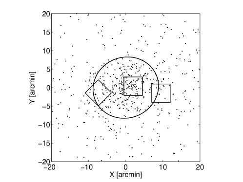
Figure 2: Distribution of our GMOS target fields in CVnI. The data points show the positions of stars satisfying our CMD selection cut. The slight excess of stars in the region $-10<X<10$ and $-5<Y<5$ indicates the location of the main body of CVnI. The ellipse shows the half-light radius of the system, with semi-major axis $8.9$ arcmin (Martin et al., 2008b).

The GMOS detector consists of three adjacent CCDs. As the dispersion axis of the slits is perpendicular to the spaces between the CCDs, the spectra contain gaps corresponding to the inter-CCD gaps. In order to achieve continuous wavelength coverage throughout the spectral region of interest, each mask was observed in two configurations with different central wavelengths ($855$nm and $860$nm). All observations were taken using the R831+_G5302 grating and CaT_G0309 filter, with 2$\times$4 spectral and spatial binning, respectively. The spectra thus obtained have a nominal resolution of 3600. The three fields were observed for a total of 10,800s, 9,000s and 12,600s, respectively, with the observations divided into individual exposures of 1800s to facilitate cosmic ray removal.

The raw data were reduced using the standard gemini reduction package which is run within the Image Reduction and Analysis Facility (IRAF) environment. All data were first bias subtracted and flat-field corrected. The individual spectral traces were identified from flat field images (obtained using Quartz halogen continuum lamp exposures). The wavelength calibration of the spectra was performed using CuAr lamp exposures adjacent in time to the science exposures as calibration frames. The typical r.m.s. uncertainty in the wavelength calibration, obtained by fitting a polynomial to the line positions in the CuAr spectra, was $0.01$Å, which corresponds to a velocity error of $\sim 0.4$ km s^-1 at a wavelength of $860$nm. This wavelength solution was then applied to the reduced science spectra. Sky subtraction was performed by using the sky flux in the regions of the slit not dominated by light from the target to estimate the sky spectrum. Finally, the object spectra were extracted from the CCD images using a fifth order Chebyshev polynomial fit. Figure 3 shows examples of a good quality spectrum (top panel), a low quality spectrum (middle panel), and typical quality spectrum (bottom).

Figure 3: Three sample spectra for stars of magnitude i$=19.7$ (top), i$=20.6$ (middle) and i$=20.1$ (bottom). The quality of the spectrum in the bottom panel is typical of the majority of our stars.

2.2 Velocities

The velocities of the stars were calculated using the fxcor task in IRAF to cross-correlate the stellar spectral lines with the lines in a template Ca triplet spectrum. The synthetic template consisted of three Gaussian lines at the wavelengths of the Ca triplet lines, whose widths were chosen to match those typical of RGB stars. We first cross-correlated the individual science exposures as a preliminary diagnostic of whether any spectra were obviously anomalous and should be excluded. As none of the spectra seemed to have serious problems, all frames were used in the velocity calculations and we combined all heliocentric-corrected exposures of the same mask together in order to increase the signal-to-noise.

The fxcor task returns estimated velocity uncertainties which are based on the Tonry-Davis Ratio for the fitted cross-correlation peak. These errors are often found not to be an accurate reflection of the true uncertainties (see e.g. Kleyna et al., 2002; Muñoz et al., 2005). In order to estimate the actual uncertainty in our velocity determinations, we measured separately the velocities $v_{1}$ and $v_{2}$ for the spectra with central wavelengths 855nm and 860nm, respectively. We combined these estimates to obtain the mean velocity for each star $\overline{v}=0.5(v_{1}+v_{2})$ and defined a $\chi^{2}$ statistic via

$$\chi^{2}=\frac{(v_{1}-\overline{v})^{2}}{(dv_{1})^{2}}+\frac{(v_{2}-\overline{v})^{2}}{(dv_{2})^{2}},$$ (1)

where $dv_{1}$ and $dv_{2}$ are the formal errors returned by fxcor. We then rescaled the velocity errors in our sample by a factor $f$ so that the sum of equation 1 over all stars was $2N$, where $N$ is the size of the velocity sample. Finally, using the rescaled errors, we calculated $P(\chi^{2})$ for each star, using the routine gammq from Numerical Recipes (Press et al., 1991). The final velocities and errors are given in Table 1. Following the error rescaling, only one star was found to have an extremely low value of $P(\chi^{2})$ ($<10^{-4}$). As Table 1 shows, this star also has the largest velocity in the sample and a relatively large estimated velocity error, possibly due its low signal-to-noise ratio, and we therefore excluded it from our final sample. We also excluded one star which has very different radial velocity $v_{R}=-39.1$ km s^-1 compared to mean velocity of the rest of our target stars ($25.8\pm 0.3$ km s^-1; see Section 2.4). Figure 4 shows the velocity histogram for our final sample consisting of $26$ stars. We note that our sample includes 10 stars from the Ibata et al. (2006) and Martin et al. (2007) sample and Figure 5 is a histogram representing the difference between the velocities of these stars from both studies in terms of their $1\sigma$ measurement uncertainties. Thus, we calculate $\Delta\rm v/\langle\sigma\rangle$ as $(v_{Keck}-v_{GMOS})/\sqrt{dv^{2}_{Keck}+dv^{2}_{GMOS}}$, after applying a velocity shift of -3.4 km s^-1 to our estimates in order to bring the median of the two data sets together. The plot shows that apart from the two outliers, at 8.6 and 4.6$\sigma$, with very different velocities in the two sets, the differences are normally distributed. The outliers are possibly stars in binary systems which have changed their velocity between the two observations. The Ibata et al. (2006) data were taken in May 2006, i.e. around ten months earlier than our data. The observed velocity differences of $8-10$km s^-1 over this baseline are consistent with tight binary orbits.

2.3 Metallicities

It is now well-established that the line strength of the near-infrared Ca triplet lines in the spectrum of an RGB star can be used to estimate the [Fe/H] of the star (e.g. Armandroff & Zinn, 1988; Armandroff, 1991; Carrera et al., 2007; Bosler et al., 2007). We note that the accuracy of this method may be less reliable when extrapolating below metallicities of $\sim-2.2$ where globular cluster calibrators are missing (Koch et al., 2008), although comparisons of high-vs-low resolution data by Battaglia et al. (2008) have shown that CaT-based estimates may be correct down to [Fe/H] $\sim-3$. In practice, we normalized the spectra using a seventh order Legendre polynomial, fitted each of the triplet lines using a Penny function (see Cole et al., 2004), and integrated the profile over the standard band passes of Armandroff & Zinn (1988). The final [Fe/H] metallicities, on the scale of Carretta & Gratton (1997), were calculated using the calibration of  Rutledge et al. (1997a; 1997b), namely

$${\rm[Fe/H]}=-2.66+0.42[\Sigma W+0.64({\rm V}-{\rm V}_{\rm HB})],$$ (2)

where we parameterised the line strength of the Ca triplet as

$$\Sigma W=0.5*w_{1}+w_{2}+0.6*w_{3},$$ (3)

where $w_{1}$, $w_{2}$ and $w_{3}$ are the widths of the individual lines. In Eq. 2, V is the V-band magnitude of the star, and V_HB is the magnitude of the horizontal branch of the system. For the latter, we used a value of $\rm V_{HB}=22.4$, obtained by visual inspection of the (V-I,V) colour-magnitude diagram of CVnI. We note that this is very similar to the value of $\rm V_{HB}=22.5$ used by Martin et al. (2008a). The uncertainty of $\sim 0.1$ magnitudes in V_HB gives rise to a negligible additional uncertainty in our [Fe/H] estimates. The random errors on the [Fe/H] metallicities were calculated using the formalism of Cayrel (1988) for the errors on the single line widths and are based on the spectral signal-to-noise ratio. These were then propagated through the calibration equations, accounting for photometric errors. The final metallicity estimates are given in Table 1. Figure 6 shows the distribution of velocity versus [Fe/H] for our CVnI sample. The error-weighted mean [Fe/H] is $-1.9\pm 0.02$ compared to the value of $-2.09\pm 0.02$ found by  Simon & Geha (2007). We note that all previous studies of CVnI have found a significant spread in [Fe/H], of order 0.5 dex (Ibata et al., 2006; Simon & Geha, 2007; Kirby, 2008), and our value thus lies within the range of previous estimates. As the figure shows, there appear to be no obvious correlations between velocity and [Fe/H] in our sample.

Figure 4: Velocity histogram for our data set of 26 likely members of CVnI. Two obvious velocity outliers (at $44$ km s^-1 and $-39.1$ km s^-1) have been excluded in from the figure.

Figure 5: Histogram of the normalised differences in estimated velocity for the ten stars observed both by us and Ibata et al. (2006). Differences have been normalised by the combined error from the two estimates (see text for details). Apart from the two significant outliers, the distribution is close to the overplotted Gaussian.

Figure 6: Line of sight velocity versus [Fe/H] for our sample of likely CVnI members. The two obvious velocity outliers have been excluded.

$\alpha$ (J2000)	$\delta$ (J2000)	V	I	g	i	$v_{\rm r}$ (km s-1)	$dv_{\rm r}$	$\sum$W	d$\sum$W	[Fe/H]	$d$[Fe/H]
$13\,28\,10.07$	$+33\,33\,41.6$	$20.2$	$19.2$	$20.7$	$19.7$	$29.2$	$1.7$	$3.12$	$0.07$	$-1.93$	$0.10$
$13\,28\,10.31$	$+33\,33\,06.0$	$19.8$	$18.6$	$20.3$	$19.1$	$39.9$	$1.6$	$3.02$	$0.05$	$-2.09$	$0.11$
$13\,28\,16.78$	$+33\,32\,54.0$	$20.6$	$19.6$	$21.1$	$20.0$	$21.9$	$2.4$	$2.83$	$0.08$	$-1.95$	$0.10$
$13\,28\,15.00$	$+33\,32\,01.6$	$20.8$	$19.9$	$21.3$	$20.3$	$30.4$	$2.1$	$2.72$	$0.14$	$-1.93$	$0.11$
$13\,28\,18.31$	$+33\,33\,17.3$	$20.8$	$19.9$	$21.2$	$20.4$	$14.5$	$1.9$	$2.96$	$0.11$	$-1.84$	$0.10$
$13\,28\,08.49$	$+33\,33\,29.4$	$21.2$	$20.2$	$21.5$	$20.6$	$35.2$	$2.4$	$2.94$	$0.19$	$-1.76$	$0.12$
$13\,28\,08.82$	$+33\,34\,41.2$	$19.9$	$18.8$	$20.4$	$19.2$	$25.9$	$1.5$	$3.22$	$0.05$	$-1.97$	$0.11$
$13\,28\,10.35$	$+33\,34\,27.7$	$20.2$	$19.1$	$20.7$	$19.5$	$24.4$	$1.5$	$3.55$	$0.06$	$-1.76$	$0.11$
$13\,28\,16.23$	$+33\,34\,09.9$	$20.2$	$19.0$	$20.7$	$19.5$	$24.8$	$1.6$	$3.81$	$0.10$	$-1.66$	$0.12$
$13\,28\,11.31$	$+33\,35\,06.1$	$20.8$	$19.7$	$21.3$	$20.2$	$21.9$	$1.8$	$3.77$	$0.15$	$-1.51$	$0.12$
$13\,28\,07.19$	$+33\,36\,05.4$	$20.2$	$19.1$	$20.7$	$19.5$	$23.8$	$1.0$	$2.51$	$0.08$	$-2.19$	$0.10$
$13\,28\,13.74$	$+33\,35\,55.6$	$19.7$	$18.5$	$20.2$	$18.9$	$21.3$	$1.3$	$3.19$	$0.06$	$-2.05$	$0.11$
$13\,28\,24.02$	$+33\,35\,32.7$	$21.0$	$20.1$	$21.4$	$20.5$	$44.0$	$3.2$	$2.23$	$0.18$	$-2.09$	$0.11$
$13\,27\,38.76$	$+33\,32\,55.3$	$20.0$	$18.8$	$20.5$	$19.3$	$12.3$	$1.4$	$2.65$	$0.05$	$-2.19$	$0.10$
$13\,27\,33.80$	$+33\,32\,57.3$	$20.8$	$19.7$	$21.2$	$20.1$	$31.9$	$1.4$	$3.20$	$0.09$	$-1.75$	$0.10$
$13\,27\,28.41$	$+33\,33\,26.3$	$20.8$	$19.7$	$21.3$	$20.2$	$-39.1$	$2.0$	$4.26$	$0.13$	$-1.29$	$0.12$
$13\,27\,28.29$	$+33\,32\,10.6$	$19.6$	$18.3$	$20.2$	$18.8$	$26.9$	$1.6$	$4.06$	$0.13$	$-1.70$	$0.13$
$13\,27\,30.35$	$+33\,32\,04.3$	$21.1$	$20.1$	$21.5$	$20.6$	$15.6$	$2.1$	$3.01$	$0.13$	$-1.73$	$0.11$
$13\,27\,30.78$	$+33\,29\,38.9$	$20.6$	$19.6$	$21.1$	$20.1$	$19.8$	$1.8$	$4.12$	$0.14$	$-1.41$	$0.12$
$13\,27\,31.21$	$+33\,29\,59.2$	$19.3$	$17.9$	$19.9$	$18.4$	$14.8$	$1.1$	$4.01$	$0.05$	$-1.81$	$0.12$
$13\,27\,16.19$	$+33\,32\,22.2$	$20.1$	$18.9$	$20.6$	$19.4$	$21.0$	$1.2$	$2.98$	$0.05$	$-2.02$	$0.10$
$13\,28\,52.91$	$+33\,29\,26.0$	$19.8$	$18.5$	$20.3$	$19.0$	$31.3$	$1.7$	$3.11$	$0.06$	$-2.07$	$0.11$
$13\,28\,46.21$	$+33\,30\,49.7$	$21.1$	$20.1$	$21.4$	$20.5$	$35.9$	$1.9$	$3.29$	$0.18$	$-1.67$	$0.12$
$13\,28\,50.64$	$+33\,31\,20.9$	$20.0$	$18.8$	$20.5$	$19.3$	$42.1$	$1.6$	$2.93$	$0.11$	$-2.07$	$0.11$
$13\,28\,50.29$	$+33\,32\,31.6$	$19.7$	$18.4$	$20.3$	$18.9$	$37.0$	$1.3$	$4.24$	$0.13$	$-1.60$	$0.13$
$13\,28\,45.29$	$+33\,31\,35.1$	$21.0$	$20.0$	$21.4$	$20.4$	$37.1$	$2.1$	$3.05$	$0.15$	$-1.76$	$0.11$
$13\,28\,53.47$	$+33\,33\,22.5$	$20.7$	$19.7$	$21.1$	$20.1$	$22.1$	$1.9$	$2.12$	$0.14$	$-2.21$	$0.10$
$13\,28\,44.26$	$+33\,34\,11.8$	$19.5$	$18.3$	$20.0$	$18.7$	$31.0$	$1.7$	$2.47$	$0.08$	$-2.40$	$0.12$

Table 1: Summary of properties of our CVnI data. Columns give: (1) Right ascension; (2) Declination; (3,4) V and I magnitudes, calculated from SDSS photometry using the transformations of Lupton (2005: http://www.sdss.org/dr4/algorithms/sdssUBVRITransform.html#Lupton). Lupton derived these equations by matching photometry from SDSS Data Release 4 to Stetson’s published photometry; (5,6) SDSS g, i magnitudes; (7,8) radial velocity and error, in km s^-1; (9,10) combined equivalent width of Ca triplet lines, with error, obtained using equation 3; (11,12) estimated metallicity [Fe/H], with error, obtained using equation 2. Note that one star ($v=-39.1$ km s^-1) is a clear outlier from the mean velocity of $v=25.8\pm 0.3$ km s^-1. A second outlier has $v=44$ km s^-1 and also a relatively large error of $dv=3.2$ km s^-1 for our sample. We therefore exclude these two stars from our analysis.

2.4 Mass Calculation

In order to estimate the mass of CVnI, we calculate the velocity dispersion of the system using the new velocity set that we obtained in the previous section. We use a maximum likelihood method  (e.g. Kleyna et al., 2004) to calculate the velocity dispersion and the mean velocity of our data. We apply an iterative $3\sigma$ cut in velocity - however, we note that this did not remove any stars (ie. it converged after a single iteration). Based on the CMD in Figure 1, we do not expect significant foreground contamination in our velocity sample, and we therefore use all 26 of our stars when estimating the dispersion. We find a dispersion of $\sigma=7.9^{+1.3}_{-1.1}$ km s^-1 and a mean velocity of $v=25.8\pm 0.3$ km s^-1. The latter is somewhat smaller than the value of $v=30.9\pm 0.6$ km s^-1 found by Simon & Geha (2007). Ibata et al. (2006) found dispersions of $13.9$ km s^-1 and $0.5$ km s^-1 for the two populations they identified. As we discuss below, we do not find evidence of multiple populations in our data and we therefore quote only a single value for the dispersion.

Following  Ibata et al. (2006) we use our dispersion measurement to constrain the mass of CVnI. In order to proceed we need to parameterise the spatial distribution of our data. We assume that our tracer population is drawn from a Plummer distribution and we find the scalelength for which the likelihood of the positions of our tracer data set is maximised. Based on the positions of our tracer stars only, we find a Plummer scalelength of $a=4.62$ arcmin, which is smaller than the value of $8.5\pm 0.5$ arcmin found by  Zucker et al. (2006a) and $8.9\pm 0.4$ arcmin found by  Martin et al. (2008b) for the full stellar distribution. The mass is then calculated using the isotropic Jeans equation  (Binney & Tremaine, 1987, eq. 4.56), under the additional assumption of spherical symmetry.

We find a mass of $4.4^{+1.6}_{-1.1}\times 10^{7}M_{\odot}$ within the volume probed by our data (i.e. out to a radius of $11$ arcmin). The mass-to-light ratio is calculated assuming a luminosity of $\mbox{L}=(2.3\pm 0.3)\times 10^{5}$ L_⊙  (Martin et al., 2008b). Assuming symmetric errors we find $\mbox{M/L}=192\pm 76\,$M_⊙/L_⊙. If we take the value of the scalelength reported by Zucker et al. (2006a) to be that of our tracers, we obtain a mass of $3.3^{+1}_{-2}\times 10^{7}M_{\odot}$. We note that both these estimates are larger than the mass of M$=(2.7\pm 0.4)\times 10^{7}M_{\odot}$ reported by  Simon & Geha (2007) using their larger data set. The difference is probably due to our assumption of a constant velocity dispersion profile, while the assumption of mass-follows-light was implicitly made by those authors.  Ibata et al. (2006) obtained two very different mass estimates using the distinct populations which they identified in their data. An important point to keep in mind while dealing with small data sets is that the Jeans equations remain valid for density-weighted averages of the spatial distributions, velocity dispersion profiles and velocity anisotropy profiles of multiple tracer populations (Strigari et al., 2007). Thus, it is legitimate to use a data set which may contain multiple sub-populations when estimating the mass of the system. As long as all sub-populations are in dynamical equilibrium, this estimate will be more reliable than the noisier estimates based on the smaller, individual populations.

3 Sub-populations

3.1 Canes Venatici I

As we noted above,  Ibata et al. (2006) identified two kinematically distinct populations in CVnI. Given the potential importance of sub-populations in dSphs discussed in the introduction, we now investigate whether our data exhibit any evidence of multiple populations. Although Fig.6 shows a wide scatter in the abundances that might be due to an extended star formation period, no clear signature of distinct sub-populations is seen. In order to confirm this visual impression more quantitatively, we fitted our velocity distribution with multiple Gaussians and tested the significance of the fits using Monte Carlo realisations of our data. Our approach, which is essentially a likelihood ratio test, is similar to the KMM test  (Ashman, Bird, & Zepf, 1994) which is designed to detect multiple Gaussian populations with different means and dispersions within a single data set, although unlike the KMM test we do not include a determination of which sub-population the individual stars belong to.

The first step of this process was to fit a single Gaussian to our velocity data. We then repeated the fit for a two-Gaussian model in which a fraction $f$ of the data belonged to a population with mean $\overline{v_{1}}$ and dispersion $\sigma_{1}$, and the remaining data had mean $\overline{v_{2}}$ and dispersion $\sigma_{2}$. As expected, the two-Gaussian model yielded higher likelihoods. In order to determine whether this was only due to the increased number of fitting parameters or was a real detection, we tested the significance of the results with artificial data. To do this, we generated 1000 data sets of 26 stars drawn from a single Gaussian and calculated the improvement of the fit with a two-Gaussian model. The distribution of probability ratios $\Delta P$ is shown in Figure 7. The value we obtained for our CVnI data is shown as the single dot in the Figure (upper panel). As this point coincides with the peak obtained by fitting two Gaussians to artificial data consisting of a single population, we conclude that we do not see evidence for a second population in our data. The panel on the bottom of figure 7 shows the equivalent test for the  Ibata et al. (2006) data (where we have taken the data for their 26 stars with S/N $>15$ as listed in Table 2 of Martin et al., 2007). In this case the improvement is larger than would be expected to arise by chance in a single-Gaussian data set. We note that a similar result is obtained when the two data sets are combined. Therefore we conclude that there is evidence of a second population containing $40$ per cent of the total number of stars, in the Ibata et al. (2006) data set, at almost the $3\sigma$ confidence level. We find that the dispersions of these populations are $0.6$ km s^-1 and $13.6$ km s^-1, respectively. Although these values are similar to those found by Ibata et al. (2006), we note that the populations we have identified may be different to those in that paper, as in that case the separation of the populations included an explicit velocity cut.

Figure 7: Distribution of likelihood ratios $\Delta P=\log P_{2}-\log P_{1}$ between a single-Gaussian fit ($P_{1}$) and a two-Gaussian fit ($P_{2}$) to 1000 Monte Carlo realisations of 26 stars drawn from a single Gaussian distribution. The single dots indicate the values obtained for our GMOS-N data (upper panel) and the Keck data of Ibata et al. (2006) (bottom panel). Although there is no evidence of multiple populations in our data, a sub-population containing a fraction of $40$ per cent of the stars is detected in the Ibata et al. (2006) data. See text for a detailed discussion.

3.2 Detectability

Figure 8: Histograms illustrating the detectability of sub-populations as a function of sample size. The two histograms in each panel show the distribution of likelihood differences $\Delta P=\log P_{2}-\log P_{1}$ between a single-Gaussian fit ($P_{1}$) and a two-Gaussian fit ($P_{2}$) for data sets having either a single population (dashed histogram) or two equal-sized populations (solid histogram). The velocity error is constant: $dv=2$ km s^-1. The total number of stars is 120 in the left panel, 60 in the middle panel and 30 in the right panel. As expected, the histograms merge together as the number of stars decreases and the detection of a sub-population becomes more difficult.

Having considered our CVnI data set, in this section we investigate the more general question of when sub-populations can be reliably detected in small kinematic data sets. A limitation of our study is that, for simplicity, we are working entirely with Gaussian populations. However, our results will be conservative in the sense that mixtures of non-Gaussian populations are likely to be more difficult to disentangle.

The detectability of a sub-population depends on i) the total number of stars in the data set; ii) the fraction of stars in the sub-population; iii) the difference in velocity dispersion between the populations; iv) the observational errors on the velocities. We investigate the importance of each of these in turn.

The total number of the stars is crucial for the detection of multiple populations. Figure 8 shows three tests done with data sets of $N=120$, $60$ and $30$ stars. In each panel a comparison is made between data sets that have either a single population or two populations containing equal numbers ($N/2$) of stars. Motivated by the case of CVnI, we consider data sets having two sub-populations with $\sigma=13$ km s^-1 and $\sigma=1$ km s^-1. The two populations are thus clearly distinct and we are thus isolating the effect of the sample size in the result. In Figure 8, we plot the improvement in probability obtained using a two-Gaussian fit to the single and double populations as dashed and solid histograms, respectively. We determine the $1\sigma$ and $3\sigma$ range of the distribution of values obtained from the single population (control) sample , and define a ($1\sigma$) $3\sigma$ detection of a sub-population to be one in which $\Delta P$ is larger than the $1\sigma$ ($3\sigma$) limits of the control sample. Although the difference between the dispersions is large, as we reduce the sample size, the significance of the detection of multiple populations decreases, as would be expected. Nevertheless, even for $N=30$ stars, in 34.8 per cent (97.5 per cent) of cases, the subpopulation is detected at the $3\sigma$ ($1\sigma$) confidence level.

The next parameter that we study is the fractional size of the sub-populations. This is important for the CVnI populations, since it is possible that a cold population in the centre could have been missed in our sample if it contained a smaller number of stars. Our preliminary tests showed that a cold population could not be detected even in a large sample if it only made up $\sim 0.1$ of the total number of stars. Figure 9 shows results for cold populations with fractional sizes $f=0.3$ , $f=0.5$ and $f=0.7$. In this test, the dispersions of the sub-populations are $13$ km s^-1 and $1$ km s^-1 and the velocity error is $2$ km s^-1. For $120$ stars, a $3\sigma$ detection was made for all the samples with a cold population of fractional size $f=0.5$ and $f=0.7$. We found (see Figure 9) that when the cold population has a smaller fractional size in the sample i.e. $f=0.3$, it was detected in 75.1 per cent (99.8 per cent) of cases at the $3\sigma$ ($1\sigma$) level. It is thus easier to detect a sub-population if its dispersion is larger than that of the main population, rather than a cold sub-population.

We next consider the impact of velocity errors on our ability to detect multiple populations with similar velocity dispersions. The sub-populations in this case have $\sigma_{1}=7$ km s^-1 and $\sigma_{2}=4$ km s^-1. As Figure 10 shows, decreasing the errors from $dv=2$ km s^-1 to $dv=1$ km s^-1 gives rise to a small change in the distribution of $\Delta P$ values. However, this does not lead to a significant increase in the probability of detecting the multiple populations. We therefore conclude that velocity errors at the $1-2$ km s^-1 (similar to the CVnI data) do not affect our ability to identify sub-populations.

Finally, to see the effect of the difference between the velocity dispersions of the populations we investigate samples in which the main population has a dispersion of $15$ km s^-1 while the cold sub-populations have dispersions ranging from $\sigma=1$ km s^-1 to $14$ km s^-1. We consider two sample sizes, with a total number of either $120$ or $60$ stars. We find that even for a relatively large sample of stars ($N=120$), a $3\sigma$ detection is possible for all the samples only when $\sigma_{1}/(\sigma_{1}-\sigma_{2})\leq 1.1$, i.e. when the velocity dispersions of the individual populations are $\sigma_{1}=15$ km s^-1 and $\sigma_{2}=1$ km s^-1. A $1\sigma$ level detection is possible for all 1000 samples for $\sigma_{1}/(\sigma_{1}-\sigma_{2})\leq 1.3$, in which case the sub-populations’ dispersions are $\sigma_{1}=15$ km s^-1, $\sigma_{2}=3$ km s^-1. However populations with $\sigma_{1}/(\sigma_{1}-\sigma_{2})\leq 1.4$ and $\sigma_{1}/(\sigma_{1}-\sigma_{2})\leq 1.9$ can be detected at $3\sigma$ and $1\sigma$ levels for 68 per cent of the 1000 samples. For a smaller sample ($N=60$), a $3\sigma$ detection for all samples is not possible for even the largest ratios of of $\sigma_{1}/\sigma_{2}$. In this case $3\sigma$ and $1\sigma$ detections for 68 per cent of the samples require $\sigma_{1}/(\sigma_{1}-\sigma_{2})\leq 1.3$ and $\sigma_{1}/(\sigma_{1}-\sigma_{2})\leq 1.7$ respectively. We note that the claimed CVnI populations in  Ibata et al. (2006) have an even more extreme dispersion difference $\sigma_{1}/(\sigma_{1}-\sigma_{2})=1.04$. A Monte Carlo experiment with 26 stars and this dispersion ratio shows that in this case populations can be identified with $3\sigma$ confidence in 90.5 per cent of the samples. Table 2 summarises our results for the full range of dispersions ratios we have considered.

Figure 9: Histograms illustrating the effect of the relative sizes of the populations. As in previous figures, the histograms show the distribution of likelihood differences $\Delta P=\log P_{2}-\log P_{1}$ between a single-Gaussian fit ($P_{1}$) and a two-Gaussian fit ($P_{2}$) to the data sets. The histograms are plotted for a single population (dot-dashed line), and for double populations including a cold sub-population consisting of 30 per cent (dotted), 50 per cent (dashed line) and 70 per cent (solid line) of the total sample of 120 stars. See text for a discussion.

∑

Figure 10: Histograms illustrating the effect of velocity errors on the detection of sub-populations with similar velocity dispersions. The total number of stars is 120 and the sub-populations contain equal numbers of stars. In each case, the double-populated sample with $\sigma_{1}=7$ km s^-1 and $\sigma_{2}=4$ km s^-1 is shown by the solid-line histogram and compared to a single population system with $\sigma=7$ km s^-1, shown as a dotted histogram. In the top panel, the velocity errors for both histograms are $dv=2$ km s^-1. As this error is relatively large compared to the difference in the dispersion, in the bottom panel we repeat the same experiment with $dv=1$ km s^-1.

$\sigma_{1}/(\sigma_{1}-\sigma_{2})$	N	$N>\sigma$	$\rm N>3\sigma$
	$120$ stars	$1000$	$1000$
$1.1$	$60$ stars	$1000$	$984$
	$120$ stars	$1000$	$999$
$1.2$	$60$ stars	$999$	$895$
	$120$ stars	$1000$	$963$
$1.3$	60 stars	$989$	$685$
	$120$ stars	$997$	$782$
$1.4$	60 stars	$946$	$397$
	$120$ stars	$966$	$480$
$1.5$	60 stars	$851$	$189$
	$120$ stars	$874$	$203$
$1.7$	60 stars	$711$	$82$
	$120$ stars	$738$	$72$
$1.9$	60stars	$572$	$31$
	$120$ stars	$562$	$28$
$2.1$	60 stars	$451$	$12$
	$120$ stars	$424$	$5$
$2.5$	60 stars	$347$	$4$
	$120$ stars	$313$	$4$
$3.$	60 stars	$276$	$2$
	$120$ stars	$227$	$1$
$3.8$	60 stars	$228$	$2$
	$120$ stars	$193$	$0$
$5$	60 stars	$195$	$1$
	$120$ stars	$160$	$0$
$7.5.$	60 stars	$174$	$1$
	$120$ stars	$145$	$0$
$15$	60 stars	$154$	$1$

Table 2: Confidence limits for the detection of sub-populations with different kinematics. Columns are: (1) Ratio of main velocity dispersion $\sigma_{1}$ to the difference between the populations $\sigma_{1}-\sigma_{2}$; (2) total number of stars in the data set; (3) Number of two-population samples for which $\Delta P$ is greater than the $1\sigma$ upper limit of $\Delta P$ obtained from single-population samples; (4) Number of two-population samples for which $\Delta P$ is greater than the $3\sigma$ upper limit of $\Delta P$ obtained from single-population samples. We compare populations of 60 and 120 stars containing two sub-populations. In each case $\sigma_{1}=15$ km s^-1 while $\sigma_{2}$ lies in the range $1$ km s^-1 to $14$ km s^-1. Each dispersion ratio has been tested for 1000 data sets.

4 Conclusions

In this paper, we have presented a new data set of velocities and metallicities for the Canes Venatici I (CVnI) dSph based on spectra taken with the GMOS-North spectrograph. A maximum likelihood fit to the velocity distribution yields a mean velocity of $v=25.8\pm 0.3$ km s^-1 and a dispersion of $\sigma=7.9^{+1.3}_{-1.1}$ km s^-1. Assuming a constant, isotropic velocity dispersion and a Plummer profile for the mass distribution, we find a mass of $4.4^{+1.6}_{-1.1}\times 10^{7}M_{\odot}$ in the volume where our tracer stars are located. Although this value is larger than the value $2.7\pm 0.4\times 10^{7}M_{\odot}$ calculated by  Simon & Geha (2007),this is most likely due to the assumptions made for our models and the distribution of our particular subsets of stars.

One of the original aims of our study was to investigate the claimed multiple stellar populations in CVnI. As we discussed above, the two previous studies by  Ibata et al. (2006) and  Simon & Geha (2007) did not agree on the existence of a cold sub-population in CVnI. The two populations found in the former study were puzzling as they led to two different mass estimates. The authors suggested that this might indicate that the system had recently accreted a younger population and was not yet in equilibrium.

In this paper we looked for evidence of multiple populations in our data under the assumption that each population was Gaussian. Based on this analysis, we concluded that there was no reason to suspect the presence of a second population in our data. We also applied our analysis to the Ibata et al. (2006) data where we found evidence of a statistically significant sub-population with a dispersion of $\sigma=0.6$ km s^-1 (compared to $\sigma=13.6$ km s^-1 for the main population).

Our analysis suggests that there is a qualitative difference between our data and those of Ibata et al. (2006). Although further data would be necessary to resolve this issue, we note that the spatial distributions of these two data sets are different, which could potentially account for the differences in the detected populations. However, our central field is centred close to the blue/young star population which Martin et al. (2008a) find in their photometry from the Large Binocular Telescope, and which they identify with the cold population of Ibata et al. (2006). The exact fraction of stars in each population found by Martin et al. (2008a) is currently unclear, however, and so it is possible that we have not picked up any stars associated with the cold population.

We have also carried out a study of the detectability of sub-populations in small kinematic data sets. Under the assumption of Gaussian populations, we studied the effects of four parameters. We obtained confidence limits for the detection of sub-populations in samples with different numbers of stars, different population ratios and velocity dispersions. We found that reasonable errors on the observed velocities do not affect the detectability of the sub-populations. For a given sample size, our ability to detect two populations increased as the ratio of their dispersions $\sigma_{1}/\sigma_{2}$ increased. However, even for large $\sigma_{1}/\sigma_{2}$ and equal population size, a sample of 30 stars yielded a $3\sigma$ detection in only $\sim 35$ per cent of cases. As expected, for larger sample sizes, this detection rate was significantly higher. We also showed that a cold population needs to constitute a larger fraction of the total sample than is required to detect a hot sub-population. This suggests that the robust detection of the sub-populations associated with any surviving sub-haloes within a dSph would require samples of many hundreds of velocities. In this case, localised substructures could be detected by windowing the data, provided that a window whose spatial size coincided with plausible sub-halo scales would contain a sample of at least 100 stars. As such data sets are now becoming available for many of the larger dSphs, this test may soon be feasible. We note that the claim of multiple global populations in Sculptor (Tolstoy et al., 2004) was based on a large data set and is therefore still robust.

Finally, we note that all our significance tests were based on the assumption of Gaussian populations, which was the case for all our Monte Carlo samples. However, for real data, the true distributions will not be known, and are not necessarily well-approximated by Gaussians. It is therefore difficult in a real case to assign a robust statistical significance to a particular detection of a sub-population.

As we have shown, for small data sets, many Monte Carlo realisations do not yield significant detections of the sub-populations. In the absence of a robust estimate of the confidence level of a particular detection, or additional, independent evidence of the presence of multiple populations, we conclude that one should exercise great caution in decomposing data sets of fewer than $100$ stars into multiple populations.

References

- Armandroff (1991) Armandroff T. E., Da Costa G. S., 1991, AJ, 101, 1329
- Armandroff & Zinn (1988) Armandroff, T. A., Zinn, R., 1988, AJ, 96, 92
- Ashman, Bird, & Zepf (1994) Ashman K. M., Bird C. M., Zepf S. E., 1994, AJ, 108, 2348
- Battaglia et al. (2006) Battaglia G., et al., 2006, A&A, 459, 423
- Battaglia et al. (2008) Battaglia G., Helmi A., Tolstoy E., Irwin M., Hill V., Jablonka P., 2008, Apj, 681, 13
- Belokurov et al. (2006) Belokurov V., et al., 2006, ApJ, 647, 111
- Belokurov et al. (2007) Belokurov V., et al., 2007, ApJ, 654, 897
- Besla et al. (2007) Besla, G., Kallivayalil, N., Hernquist, L., Robertson, B., Cox, T. J., van der Marel, R. P., Alcock, C., 2007, ApJ, 668, 949.
- Binney & Tremaine (1987) Binney J., Tremaine S., 1987, “Galactic Dynamics”, Princeton University Press.
- Bosler et al. (2007) Bosler, T. L., Smecker-Hane, T. A., Stetson, P. B., 2007, MNRAS, 378, 318.
- Bovill & Ricotti (2008) Bovill, M. S., Ricotti, M., 2008, arXiv:0806.2340
- Carrera et al. (2007) Carrera, R., Gallart, C., Pancino, E., Zinn, R., 2007, AJ, 134, 1298.
- Carretta & Gratton (1997) Carretta, E.; Gratton, R. G., A&AS, 121,95.
- Cayrel (1988) Cayrel, R., 1988, IAUS, 132, 345
- Cole et al. (2004) Cole A. A., Smecker-Hane T. A., Tolstoy E., Bosler T. L., Gallagher J. S., 2004, MNRAS, 347, 367
- Diemand, Madau & Moore (2005) Diemand J., Madau P., Moore B., 2005, MNRAS, 364, 367
- Font et al. (2006) Font, A. S., Johnston, K. V., Bullock, J. S., Robertson, B. E., 2006, 2006, ApJ, 646, 886.
- Gao (2004) Gao L., White S. D. M., Jenkins A., Stoehr F., Springel V., 2004, MNRAS, 355, 819
- Gilmore et al. (2007) Gilmore G., Wilkinson M. I., Wyse R. F. G., Kleyna J. T., Koch A., Evans N. W., Grebel E. K., 2007, ApJ, 663, 948
- Harbeck et al. (2001) Harbeck D., et al., 2001, AJ, 122, 3092
- Helmi et al. (2006) Helmi A., et al., 2006, ApJ, 651, L121
- Ibata et al. (2006) Ibata R., Chapman S., Irwin M., Lewis G., Martin N., 2006, MNRAS, 373, L70
- Kallivayalil et al. (2006) Kallivayalil, N., van der Marel, R. P., Alcock, C., Axelrod, T., Cook, K. H., Drake, A. J., Geha, M., 2006, ApJ, 638,772.
- Kirby (2008) Kirby E. N., Simon J. D., Geha M., Guhathakurta P., Frebel A., 2008, ApJ, 807, arXiv:0807.1925
- Kleyna et al. (2002) Kleyna J., Wilkinson M. I., Evans N. W., Gilmore G., Frayn C., 2002, MNRAS, 330, 792
- Kleyna (2003) Kleyna J. T., Wilkinson M. I., Gilmore G., Evans N. W., 2003, ApJ, 588, L21
- Kleyna et al. (2004) Kleyna J. T., Wilkinson M. I., Evans N. W., Gilmore G., 2004, MNRAS, 354, L66
- Koch et al. (2006) Koch A., Grebel E. K., Wyse R. F. G., Kleyna J. T., Wilkinson M. I., Harbeck D. R., Gilmore G. F., Evans N. W., 2006, AJ, 131, 895
- Koch et al. (2007a) Koch, A., Wilkinson, M. I., Kleyna, J. T., Gilmore, G. F., Grebel, E K., Mackey, A. D., Evans, N.Wyn., Wyse, R. F. G., 2007a, ApJ, 657, 241.
- Koch et al. (2007b) Koch, A., Grebel, E. K., Kleyna, J. T., Wilkinson, M. I., Harbeck, D. R., Gilmore, G. F., Wyse, R. F. G., Evans, N. W., 2007b, AJ, 133, 270.
- Koch et al. (2008) Koch, A., Grebel, E. K., Gilmore, G. F., Wyse,R .F. G., Kleyna,J. T., Harbeck,D. R., Wilkinson, M. I., Evans, N. W., 2008, Aj, 135,1580.
- Łokas et al. (2008) Łokas E. L., Klimentowski J., Kazantzidis S., Mayer L., 2008, arXiv, 804, arXiv:0804.0204v2
- Marcolini et al. (2008) Marcolini, A., D’Ercole, A., Battaglia, G., Gibson, B. K., 2008, MNRAS,386, 2173
- Martin et al. (2007) Martin, N. F, Ibata, R. A., Chapman, S. C., Irwin, M., Lewis, G. F., 2007, MNRAS, 380, 281
- Martin et al. (2008a) Martin, N. F., et al., 2008a, ApJ, 672, 13.
- Martin et al. (2008b) Martin, N. F, de Jong, J. T. A., Rix, H.-W, 2008b arXiv:0805.2945v2
- Mateo (1998) Mateo M. L., 1998, ARA&A, 36, 435
- Mateo (2008) Mateo M., Olszewski E. W., Walker M. G., 2008, ApJ, 675, 201
- Moore et al. (2006) Moore B., Diemand J., Madau P., Zemp M., Stadel J., 2006, MNRAS, 368, 563
- Moore et al. (1999) Moore B., Ghigna S., Governato F., Lake G., Quinn T., Stadel J., Tozzi P., 1999, ApJ, 524, L19
- Muñoz et al. (2005) Muñoz R. R., et al., 2005, ApJ, 631, L137
- Muñoz, Majewski, & Johnston (2008) Muñoz R. R., Majewski S. R., Johnston K. V., 2008, ApJ, 679, 346
- Piatek et al. (2008) Piatek, S., Pryor, C., Olszewski, E. W., 2008, AJ, 135.1024.
- Press et al. (1991) Press, W. H., Flannery, B. P. Teukolsky, S. A, Vetterling, W. T., 1991, “Numerical Recipes in C”, Cambridge University Press
- Robertson et al. (2005) Robertson, B., Bullock, J. S., Font, A. S., Johnston, K. V., Hernquist, L., 2005, ApJ, 632, 872.
- Rutledge et al. (1997a) Rutledge G. A., Hesser J. E., Stetson P. B., Mateo M., Simard L., Bolte M., Friel E. D., Copin Y., 1997a, PASP, 109, 883
- Rutledge, Hesser, & Stetson (1997b) Rutledge G. A., Hesser J. E., Stetson P. B., 1997b, PASP, 109, 907
- Simon & Geha (2007) Simon J. D., Geha M., 2007, ApJ, 670, 313
- Shetrone et al. (2001) Shetrone, M. D., Côté, P., Sargent, W. L. W., 2001, ApJ, 548, 592.
- Stoehr et al. (2002) Stoehr F., White S. D. M., Tormen G., Springel V., 2002, MNRAS, 335, L84
- Strigari et al. (2007) Strigari L. E., Bullock J. S., Kaplinghat M., Diemand J., Kuhlen M., Madau P., 2007, ApJ, 669, 676
- Tollerud et al. (2008) Tollerud, E. J., Bullock, J. S., Strigari, L. E, Willman, B., 2008, arXiv:0806.4381
- Tolstoy et al. (2004) Tolstoy E., et al., 2004, ApJ, 617, L119
- Unavane, Wyse & Gilmore (1996) Unavane M., Wyse R. F. G., Gilmore G., 1996, MNRAS, 278, 727
- van der Marel (2002) van der Marel R. P., Alves D. R., Hardy E., Suntzeff N. B., 2002, AJ, 124, 2639
- Venn et al. (2004) Venn, K. A., Irwin, M., Shetrone, M. D.; Tout, C. A.; Hill, V; Tolstoy, E., 2004, AJ, 128, 1177.
- Walker (2006) Walker M. G., Mateo M., Olszewski E. W., Pal J. K., Sen B., Woodroofe M., 2006, ApJ, 642, L41
- Walker et al. (2007) Walker M. G., Mateo M., Olszewski E. W., Gnedin O. Y., Wang X., Sen B., Woodroofe M., 2007, ApJ, 667, L53
- Walsh, Jerjen, & Willman (2007) Walsh S. M., Jerjen H., Willman B., 2007, ApJ, 662, L83
- Willman et al. (2005) Willman B., et al., 2005, ApJ, 626, L85
- York et al. (2000) York D. G., et al., 2000, AJ, 120, 1579
- Zucker et al. (2006a) Zucker D. B., et al., 2006a, ApJ, 643, L103
- Zucker et al. (2006b) Zucker D. B., et al., 2006b, ApJ, 650, L41