The Overlapping Muffin-Tin Approximation

Abstract

We present the formalism and demonstrate the use of the overlapping muffin-tin approximation (OMTA). This fits a full potential to a superposition of spherically symmetric short-ranged potential wells plus a constant. For one-electron potentials of this form, the standard multiple-scattering methods can solve Schrödingers’ equation correctly to 1st order in the potential overlap. Choosing an augmented-plane-wave method as the source of the full potential, we illustrate the procedure for diamond-structured Si. First, we compare the potential in the Si-centered OMTA with the full potential, and then compare the corresponding OMTA $N$-th order muffin-tin orbital and full-potential LAPW band structures. We find that the two latter agree qualitatively for a wide range of overlaps and that the valence bands have an rms deviation of 20 meV/electron for 30% radial overlap. Smaller overlaps give worse potentials and larger overlaps give larger 2nd-order errors of the multiple-scattering method. To further remove the mean error of the bands for small overlaps is simple.

1 Introduction

The linear muffin-tin orbital (LMTO) method in the atomic-spheres approximation (ASA) [1, 2] has been used for over three decades as an ab initio method for electronic-structure calculations. One of the defining characteristics of this method is its small, localized [3] basis set which provides highly efficient computation and does not require crystalline symmetry [4]. Equally important is the fact that the similarity of LMTOs to atomic orbitals makes the method physically transparent. This means that it is easy to extract e.g. information about the nature of chemical bonds, the symmetry of band states, a.s.o..

The extreme speed and simplicity of the LMTO-ASA is to a large extent due to the ASA which takes the one-electron potential and charge density to be spherically symmetric inside space-filling Wigner-Seitz spheres whose overlap is neglected. This approximation is very good, not only for closely-packed solids but also for open systems in which the interstital sites have high symmetry and can be taken as centers for ”empty” Wigner-Seitz spheres containing no protons but only electrons. The diamond structure is such a case, because both its potential and charge density are are approximately spherical inside equal-sized spheres packed on a body-centered cubic (bcc) lattice. However, for open systems with atoms of different sizes and/or with low symmetry, it can be cumbersome, if not impossible to find a good ASA.

Since most systems of current interest are low-dimensional and multi-component, and since the cost of computation has followed Moors’ law for decades, the LMTO-ASA method is now mainly used to extract information about the electrons from accurate calculations which use one of the plane-wave supercell methods. These methods employ the variational principle with large plane-wave basis sets, either for the full-potential Schrödinger equation with linear augmented plane waves (LAPWs) [1, 5] or projector-augmented plane waves (PAWs) [6], or for a pseudopotential with straight plane waves [7]. In this mode of operation, one adjusts the LMTO-ASA sphere sizes and empty-sphere positions by trial and error such as to obtain the best possible agreement with the band structure obtained with an accurate method.

Attempts have been made to improve the accuracy while preserving the desirable features of the LMTO-ASA. First [8], it was realized that the multiple-scattering method of Korringa, Kohn and Rostoker (KKR) [9], the mother of all MTO methods, solves Schrödingers’ equation not only for a MT potential, that is a potential which is spherically symmetric inside non-overlapping spheres and flat ($\equiv$0) in between, but also for a superposition of spherically symmetric potential-wells to 1st order in their overlap, with no change of the formalism. This explained why the ASA had worked much better than the MT approximation (MTA) and begged for the use of even larger potential spheres. The overlapping muffin-tin approximation (OMTA), however, turned out not to work with conventional LMTOs because the energy-dependence of their envelope functions, the decaying Hankel functions, had not been linearized away in the same way as the energy-dependence of the augmenting partial waves inside the spheres, but put to a constant (e.g. =$0$). As a consequence, exact MTOs (EMTOs) with envelopes of energy-dependent, screened solutions of the wave equation had to be found, and then linearized [10]. With the resulting, so-called 3rd-generation LMTOs (LMTO3s), it became possible to solve Schrödingers’ equation for diamond-structured silicon using the OMTA without empty spheres [11]. Specifically, the ASA potential calculated self-consistently with empty spheres (and the 14% radial overlap of bcc WS spheres) was least-squares’ fitted to a superposition of potential wells centered only on the Si sites, whereafter Schrödingers’ equation was solved for this OMTA potential with the LMTO3 method. By varying the OMTA overlap, a minimum rms error of 80 meV per valence-band electron was found around 30% overlap: for smaller overlaps the OMTA-fit was worse, and for larger overlaps the $2$nd-order overlap error of the LMTO3 method dominated. This ability of the LMTO3 method to compute the band structure for an OMTA potential was not developed into a charge-selfconsistent method, despite several attempts [12, 13], but for the EMTO Greens’-function method this was done by Vitos et al. who devised a spherical-cell approximation for closely-packed alloys and demonstrated its efficiency for overlaps around $30\%$ [14]. Instead, the unique ability of the LMTO3 method to generate super-minimal basis sets through downfolding was explored, but that led to the next problem: The smaller the basis set, the longer the range of each MTO, and the stronger its energy dependence. For very small basis sets, this energy dependence may be so strong that linearization is insufficient. That problem was finally solved through the development of a polynomial approximation of general order $(N)$ in the MTO Hilbert space, and the resulting $N$MTO method [15] has now been in use for nearly ten years, in particular for generating few-orbital, low-energy Hamiltonians in studies of correlated electron systems, but always in connection with potentials generated by the LMTO-ASA.

Here, we shall present and apply the least-squares’ formalism to fit a full potential in the form delivered by any augmented plane-wave method to the OMTA form. This procedure is demonstrated for diamond-structured silicon, first by comparison of the full with the OMTA potential, and then by comparison of the full-potential LAPW and OMTA $N$MTO band structures. Our current strategy for extracting electronic information from an accurate plane-wave calculation, is thus to fit its output potential to the OMTA and then perform $N$MTO calculations for the OMTA potential. This procedure is more simple and accurate than going via the LMTO-ASA.

2 The Overlapping Muffin-Tin Approximation

In this section we shall explain the least-squares’ procedure for obtaining the OMTA to a full potential. In the first two subsections we shall present the general formulas [13], and in the last we shall present results for the specific analytic form of the full potential provided by an augmented plane-wave method.

We wish to minimize the value of mean squared deviation,

$$\Delta F=\frac{1}{\Omega}\int_{\Omega}\left[F(\mathbf{r})-\left(g+\sum\nolimits_{j}f_{j}(|\mathbf{r}-\mathbf{R}_{j}|)\right)\right]^{2}d\mathbf{r,}$$ (1)

of the the full potential, $F\left(\mathbf{r}\right),$ from its OMTA counterpart, $g+\sum\nolimits_{j}f_{j}(r_{j})$. The spherically symmetric potential wells $f_{j}(r_{j})$ vanish for $r_{j}>s_{j}$ and are centered at the sites $\mathbf{R}_{j}$ of the atoms. $\Omega$ is the (cell) volume. To be determined are thus the radial functions $f_{j}\left(r\right)$ and the constant $g,$ for given $F(\mathbf{r}),$ $\Omega,$ $\mathbf{R}_{j},$ and $s_{j}$.

2.1 Determining the spherical potential wells, $f_{j}(r)$

Variation of $\Delta F$ with respect to $f_{j}(r)$ leads to the equation:

$$0 =\frac{\delta}{\delta f_{j}(r)}\Delta F=\frac{1}{4\pi r^{2}}\int_{\Omega}\delta(|\mathbf{r}-\mathbf{R}_{j}|-r)\left(F(\mathbf{r})-g-\sum\nolimits_{j^{\prime}}f_{j^{\prime}}(|\mathbf{r}-\mathbf{R}_{j^{\prime}}|)\right)d\mathbf{r}$$

$$\equiv\theta(s_{j}-r)\left(\bar{F}^{j,r}-g\right)-f_{j}(r)-\theta(s_{j}-r)\sum\nolimits_{j^{\prime}\neq j}\bar{f}_{j^{\prime}}^{j,r}$$ (2)

where $\bar{F}^{j,r}$ and $\bar{f}_{j^{\prime}}^{j,r}$ are the averages of the respective functions over the sphere centered at site $j$ and of radius $r$. Eq. (2) thus translates into the requirement that the spherical averages of $F(\mathbf{r})-g$ and $\sum_{j^{\prime}}f_{j^{\prime}}(r_{j^{\prime}})$ around site $j$ be the same. The problem of calculating $\bar{F}^{j,r}$ for the LAPW potential will be addressed in Sec. 2.3. By reordering of the terms in Eq. (2), and evaluating the spherical averages, we obtain:

$$rf_{j}(r)=\theta(s_{j}-r)\left[r\left(\bar{F}^{j,r}-g\right)-\sum_{j^{\prime}\neq j}\frac{\theta(s_{j}+s_{j^{\prime}}-d_{jj^{\prime}})}{2d_{jj^{\prime}}}\int_{d_{jj^{\prime}}-r}^{s_{j^{\prime}}}r^{\prime}f_{j^{\prime}}(r^{\prime})dr^{\prime}\right],$$ (3)

where $d_{jj^{\prime}}=|\mathbf{R}_{j}-\mathbf{R}_{j^{\prime}}|$ is the distance between respective sites. We have assumed that $s_{j^{\prime}}<d_{jj^{\prime}},$ i.e. that a potential sphere never includes the center of another sphere (moderate overlap). Repeating the procedure for all inequivalent sites, Eq.s (3) become a set of linear integral equations which may be solved for a given $g=g_{0}$ by self-consistent iteration. The iteration can be initiated e.g. by taking $f_{j^{\prime}}(r^{\prime})=\theta(s_{j^{\prime}}-r^{\prime})\left(\bar{F}^{j^{\prime},r^{\prime}}-g\right)$ on the right-hand side of Eq. (3).

2.2 Determining the constant background, $g$

A similar expression is obtained for the optimal value of the constant $g$, namely:

$$0=\frac{\partial}{\partial g}\Delta F=\bar{F}-g-\sum\nolimits_{j}\bar{f}_{j}$$ (4)

where $\bar{F}$ and $\bar{f}_{j}$ are the volume averages of the respective functions:

$$\bar{F}=\frac{1}{\Omega}\int_{\Omega}F(\mathbf{r})d\mathbf{r,}\quad\mathrm{and}\quad\bar{f}_{j}=\frac{1}{\Omega}\int_{\Omega}f_{j}(|\mathbf{r}-\mathbf{R}_{j}|)d\mathbf{r}=\frac{4\pi}{\Omega}\int_{0}^{s_{j}}f_{j}(r)r^{2}dr$$ (5)

Just like before, Eq. (4) expresses the condition of equality of averages of the full and OMTA potentials.

We need to solve the coupled $f$ and $g$ equations. Since these are linear, we may use the superposition principle to obtain:

$$f_{j}\left(g;r\right)=f_{j}\left(g_{0};r\right)-\left(g-g_{0}\right)h_{j}\left(r\right),$$

where the ”structure functions” $h_{j}\left(r\right)$ are the solutions of the $f$-equations (3) for $F\left(\mathbf{r}\right)-g\equiv 1.$ The optimal $g$-value is thus:

$$g=g_{0}+\left(\bar{F}-g_{0}+\sum\nolimits_{j}\bar{f}_{j}\left(g_{0}\right)\right)\left/\left(1-\sum\nolimits_{j}\bar{h}_{j}\right)\right..$$

2.3 Averages of the LAPW full potential

The procedure outlined in section 2.1 requires calculation of the volume average $\bar{F},$ and the spherical averages, $\bar{F}^{j,r},$ for $r\leq s_{j}<\min_{j^{\prime}}d_{jj^{\prime}}$ around all inequivalent sites of the full potential. This task can be achieved with relative ease thanks to the analytical form of the potential delivered by an augmented plane-wave method: Space is divided into a set of atom-centered, non-overlapping augmentation spheres with radii, $a_{j},$ and the interstitial. Inside an augmentation sphere the full potential is given by the spherical-harmonics $\left(Y_{lm}\right)$ expansion:

$$F(\mathbf{r})=\sum_{lm}F_{jlm}(r_{j})Y_{lm}(\hat{\mathbf{r}}_{j})\;\;\mathrm{for}\;\;r_{j}<a_{j}$$ (6)

where $\mathbf{r}_{j}\equiv\mathbf{r}-\mathbf{R}_{j}\equiv r_{j}\,\hat{\mathbf{r}}_{j}.$ In the interstitial, the full potential is described as a linear combination of plane waves which we shall let extend throughout space:

$$F(\mathbf{r}) = \sum_{j}\theta\left(a_{j}-r_{j}\right)\sum_{lm}\left(F_{jlm}(r_{j})-\sum\nolimits_{G}F_{jlm}\left(G\right)\,j_{l}(Gr_{j})\right)Y_{lm}(\hat{\mathbf{r}}_{j})$$ (7)

$$+\sum\nolimits_{\mathbf{G}}F\left(\mathbf{G}\right)e^{i\mathbf{G}\cdot\mathbf{r}}.$$

The first term here provides the augmentation of the plane waves, i.e. it ads expression (6) and subtracts the corresponding plane-wave part inside the spheres. $\mathbf{G}\equiv G\mathbf{\hat{G}}$ are the reciprocal lattice vectors and $F\left(-\mathbf{G}\right)=F^{\ast}\left(\mathbf{G}\right)$ because $F\left(\mathbf{r}\right)$ is real. Moreover, $j_{l}$ are the spherical Bessel functions, and

$$F_{jlm}\left(G\right)\equiv 4\pi i^{l}\sum\nolimits_{\mathbf{\hat{G}}}F\left(\mathbf{G}\right)e^{i\mathbf{G}\cdot\mathbf{R}_{j}}Y_{lm}^{\ast}(\hat{\mathbf{G}}).$$ (8)

The spherical average around site $j$ is the spherical component of the potential (6) inside the augmentation sphere: $\bar{F}^{j,r}=F_{j00}\left(r\right)/\sqrt{4\pi},$ if $r<a_{j}.$ If $r>a_{j}$ and the $r$-sphere at site $j$ cuts into the augmentation-sphere at site $j^{\prime},$ the spherical average of the corresponding term in the first line of Eq. (7) is most easily evaluated when, for the spherical-harmonics expansion inside the $j^{\prime}$-sphere, we turn the $z^{\prime}$-axis to point towards $\mathbf{R}_{j},$ i.e. along the $\mathbf{\hat{d}}_{jj^{\prime}}$ direction:

$$Y_{lm}(\hat{\mathbf{r}}_{j^{\prime}})=\sum\nolimits_{m^{\prime}}D_{mm^{\prime}}^{l}\left(\mathbf{\hat{d}}_{jj^{\prime}}\right)Y_{lm^{\prime}}\left(\hat{\mathbf{r}}_{j^{\prime}}\cdot\mathbf{\hat{d}}_{jj^{\prime}}\right)\equiv\sum\nolimits_{m^{\prime}}D_{mm^{\prime}}^{l}\left(\mathbf{\hat{d}}_{jj^{\prime}}\right)Y_{lm^{\prime}}(\theta^{\prime},\varphi^{\prime}),$$

because then the integral over $\varphi^{\prime}$ selects the term with $Y_{l0}\left(\theta^{\prime},\varphi^{\prime}\right)=\sqrt{\frac{2l+1}{4\pi}}P_{l}\left(\cos\theta^{\prime}\right)$ and only the integral over $\theta^{\prime}$ remains. Including now also the spherical average of the second line in Eq. (7), the result becomes:

$$\bar{F}^{j,r} = \sum_{j^{\prime}\neq j}\frac{\theta\left(d_{jj^{\prime}}-r\right)}{2rd_{jj^{\prime}}}\sum_{l}\int_{d_{jj^{\prime}}-r}^{a_{j^{\prime}}}r^{\prime}F_{jj^{\prime}l}\left(r^{\prime}\right)P_{l}\left(\frac{r^{\prime 2}-r^{2}+d_{jj^{\prime}}^{2}}{2r^{\prime}d_{jj^{\prime}}}\right)dr^{\prime}$$ (9)

$$+\sum_{G}j_{0}\left(Gr\right)F_{j00}\left(G\right)/\sqrt{4\pi}\,,$$

where $j_{0}\left(x\right)=\sin x/x$ and

$$F_{jj^{\prime}l}\left(r^{\prime}\right)\equiv\theta\left(a_{j^{\prime}}-r^{\prime}\right)\sqrt{\frac{2l+1}{4\pi}}\sum_{m}\left[F_{j^{\prime}lm}(r^{\prime})-\sum\nolimits_{G}F_{j^{\prime}lm}\left(G\right)\,j_{l}(Gr^{\prime})\right]D_{m0}^{l}\left(\mathbf{\hat{d}}_{jj^{\prime}}\right)$$

$$=\theta\left(a_{j^{\prime}}-r^{\prime}\right)\sqrt{\frac{2l+1}{4\pi}}\left[\sum_{m}F_{j^{\prime}lm}(r^{\prime})D_{m0}^{l}\left(\mathbf{\hat{d}}_{jj^{\prime}}\right)-\sum_{G}F_{j^{\prime}l0}^{j}\left(G\right)\,j_{l}(Gr^{\prime})\right].$$

Here, $F_{j^{\prime}l0}^{j}\left(G\right)$ is given by Eq. (8) with $Y_{l0}^{\ast}(\hat{\mathbf{G}})$ substituted by $\sqrt{\frac{2l+1}{4\pi}}P_{l}\left(\hat{\mathbf{G}}\mathbf{\cdot\hat{d}}_{jj^{\prime}}\right).$

Finally, the volume average of the full potential (7) is

$$\bar{F}=\frac{\sqrt{4\pi}}{\Omega}\sum_{j}\left(\int_{0}^{a_{j}}F_{j00}(r)r^{2}dr-a_{j}^{3}\sum_{G}\frac{j_{1}\left(Ga_{j}\right)}{Ga_{j}}F_{j00}\left(G\right)\right)+F\left(\mathbf{G}\mathrm{=}\mathbf{0}\right),$$

where $j_{1}\left(x\right)=\left(\sin x-x\cos x\right)/x^{2}.$

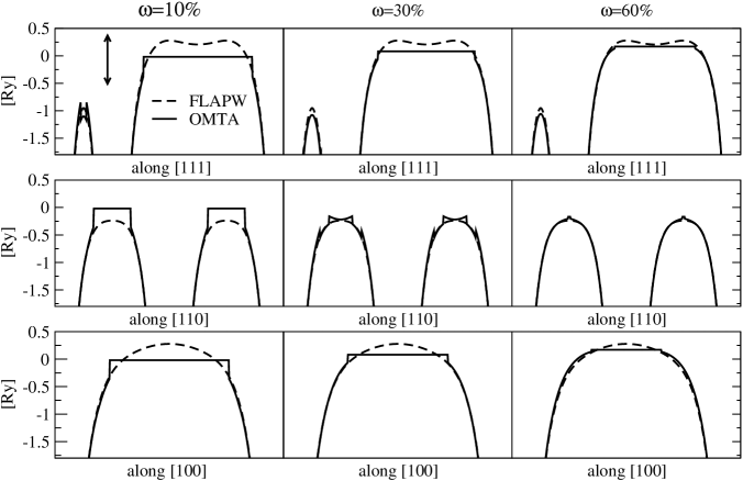
Fig. 1: Full potential for diamond-structured Si along the main crystallographic axes (dashed) and its OMTAs for 10, 30, and 60% radial overlaps (full). The double-headed arrow indicates the range of the valence bands.

3 Example: Diamond-structured silicon

In this section we shall compare the potential and band structure calculated self-consistently using the full potential LAPW method as implemented in WIEN2k [16] with respectively the OMTA to this full potential and its band structure calculated using the $N$MTO-OMTA method. As in the previous (AE)SA-vs-OMTA LMTO3 study [11], in the present full-vs-OMTA $N$MTO study we choose diamond-structured Si and OMTAs with atom-centered spherical wells in order that the study be relevant for open structures in general.

Fig. 1 compares the full potential with its OMTA for radial overlaps, $\omega\equiv(2s-d)/d,$ of 10, 30, and 60%. We see a marked improvement in the quality of the fit as the overlap, i.e. the range of $f\left(r\right),$ increases. With $60\%$ overlap the OMTA follows the full potential not only inside the potential wells, i.e. close to the nuclei where the spherical approximation is at its best, but also along the bond between the Si atoms and in the interstitial space.

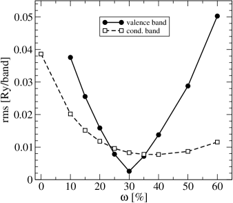
Fig. 2: Rms errors of the $N$MTO-OMTA valence and four lowest conduction bands as functions of the radial overlap, with respect to the full-potential LAPW bands.

From this, one might believe that it is always preferential to use large overlaps. But this is not so, because multiple-scattering methods are only ”self-correcting” to 1st-order in the potential overlap ($\propto\omega^{2})$ [8, 11]. For large overlaps, the errors of higher order ($\propto\omega^{4}$ and higher) outweigh the effect of the improved description of the potential. We thus expect that there exists an optimal value of the overlap which yields the best accuracy of the calculated band states. In Fig. 2 this is confirmed by explicit calculations of root mean squared (rms) error of the $N$MTO-OMTA bands with respect to their full-potential LAPW counterparts as a function of the radial overlap. The two curves are for respectively the four valence and the four lowest conduction bands. For both types of bands, the error initially decreases as a result of the improved OMTA. For the valence bands the optimum of 3 mRy/band = 20 meV/electron is reached at $30\%$ overlap, after which the error increases sharply, whereas for the conduction bands the optimum of 50 meV/e is reached at $40\%$, wherafter the multiple-scattering errors increase slowly. This difference in behaviour is due to the valence states being bonding and the conduction states antibonding, whereby the former probe the overlap region more than the latter. Whereas the rms-error curve for the conduction band is nicely flat, that of the valence band is not.

Fig. 3 shows the full-potential LAPW band structure and the $N$MTO band structures for the three OMTA potentials in Fig. 1. Excellent agreement is achieved with $30\%$ overlap for both conduction and valence bands. For smaller overlaps, the $N$MTO-OMTA bands lie to high, the valence bands in particular, and for larger overlaps they lie too low. The first point follows from the variational principle and the second from the fact that the multiple-scattering error $\propto\omega^{4}$ is negative definite. This was explained in the previous study [11], which also demonstrated the use of various corrections. The simplest of these is to remove the mean error of the energies for a group of bands, say the valence bands, by weighting the squared deviation in Eq. 1 with the charge density of those bands, and then keep the weighting in the $g$-equation only (see Sect. 2.2). Since the LAPW valence charge density has the same form as the full potential, implementation of this requires use of formulas given in Sect. 2.3. This correction will move the $N$MTO-OMTA bands down by the appropriate amount for small overlaps and, hence, considerably lower the rms-error curve for small overlaps. An elegant correction of the large-overlap errors remains to be found; the straight-forward but clumsy one is to evaluate the kinetic energy properly in the overlap region for the $N$MTO basis.

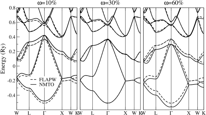
Fig. 3: Band structure of Si calculated with the full potential LAPW method (dashed) and with the $N$MTO-OMTA method for $10$, 30, and 60% radial overlap (full). The $N$MTO basis set consisted of the 9 $s$, $p,$ and $d$ Si-$N$MTOs with the $f$s downfolded and had $N$=2 with expansion energies -0.5, 0.3, and 0.6 Ry [15].

References

- [1] O.K. Andersen, Phys.Rev. B 12, 3060 (1975); D. Glötzel, B. Segall and O.K. Andersen, Solid State Commun. 36, 403 (1980).
- [2] H.L. Skriver, The LMTO Method: Muffin-Tin Orbitals and Electronic Structure, Springer-Verlag Berlin/ Heidelberg/New York/Tokyo 1984.
- [3] O.K. Andersen and O. Jepsen, Phys.Rev.Lett. 53, 2571 (1984); O.K. Andersen, O. Jepsen and D. Glötzel, Canonical Description of the Band Structures of Metals, in: Highlights of Condensed Matter Theory, edited by F. Bassani, F. Fumi and M.P. Tosi, International School of Physics ’Enrico Fermi’, Varenna, Italy (North-Holland, Amsterdam, 1985), p.59
- [4] I. Turek, V. Drchal, J. Kudrnovsky, M. Sob, and P. Weinberger, Electronic Structure of Disordered Alloys, Surfaces, and Interfaces, Kluwer Academic Publ., Boston/London/Dordrecht, 1996.
- [5] D.J. Singh, Plane waves, Pseudopotentials and the LAPW method, Kluwer Academic Publ., Dordrecht, 1994
- [6] P.E. Blöchl, Phys. Rev. B 50, 17953 (1994)
- [7] M.C. Payne, M.P. Teter, D.C. Allan, T.A. Arias and J.D. Joannopoulos, Rev. Mod. Phys. 64, 1045 (1992)
- [8] O.K. Andersen, A.V. Postnikov, and S.Yu. Savrasov, The Muffin-Tin-Orbital Point of View, in: Applications of Multiple Scattering Theory to Materials Science, edited by W.H. Butler, P.H. Dederichs, A. Gonis, and R.L. Weaver. MRS Symposium Proceedings Series, Vol. 253 (1992), p. 37.
- [9] J. Korringa, Physica 13, 392 (1947); W. Kohn and J. Rostoker, Phys. Rev. 94, 1111 (1954).
- [10] O.K. Andersen, O. Jepsen, and G. Krier, Exact Muffin-Tin Orbital Theory, in: Lectures in Methods of Electronic Structure Calculations, edited by V. Kumar, O.K. Andersen, and A. Mookerjee, (World Sci. Publ.Co., Singapore 1994), p.63.
- [11] O.K. Andersen, C. Arcangeli, R.W. Tank, T. Saha-Dasgupta, G. Krier, O. Jepsen, I. Dasgupta, Third-Generation TB-LMTO, in: Tight-Binding Approach to Computational Materials Science, eds. L. Colombo, A. Gonis, P. Turchi. MRS Symposium Proceedings Series, vol 491 (1998), p.3.
- [12] R.W. Tank and C. Arcangeli, phys. stat. sol. (b) 217, 89 (2000).
- [13] O.K. Andersen and D. Savrasov (unpublished)
- [14] L. Vitos, Phys. Rev. B 64, 014107 (2001), and Computational Quantum Mechanics for Materials Engineers: the EMTO method and applications, Springer Berlin, 2008.
- [15] O.K. Andersen, T. Saha-Dasgupta, R.W. Tank, C. Arcangeli, O. Jepsen, G. Krier, Developing the MTO formalism, in: Electronic Structure and Physical Properties of Solids. The Uses of the LMTO Method, ed. H. Dreyssé. Springer Lecture Notes in Physics. 535 (Berlin/Heidelberg 2000), p.3; O.K. Andersen and T. Saha-Dasgupta, Phys. Rev. B 62, R16219 (2000).
- [16] P. Blaha, K. Schwarz, G. Madsen, D. Kvasnicka and J. Luitz, WIEN2k, An Augmented Plane Wave + Local Orbitals Program for Calculating Crystal Properties, Karlheinz Schwarz, Techn. Universität Wien, Austria, 2001.