IPMU 08-0050
ICRR-Report-527
Non-Gaussianity from isocurvature perturbations
Masahiro Kawasakia,b, Kazunori Nakayamaa, Toyokazu Sekiguchia, Teruaki Suyamaa and Fuminobu Takahashib
aInstitute for Cosmic Ray Research,
University of Tokyo, Kashiwa 277-8582, Japan
bInstitute for the Physics and Mathematics of the Universe,
University of Tokyo, Kashiwa 277-8568, Japan
We develop a formalism to study non-Gaussianity in both curvature and isocurvature perturbations. It is shown that non-Gaussianity in the isocurvature perturbation between dark matter and photons leaves distinct signatures in the CMB temperature fluctuations, which may be confirmed in future experiments, or possibly, even in the currently available observational data. As an explicit example, we consider the QCD axion and show that it can actually induce sizable non-Gaussianity for the inflationary scale, GeV.
1 Introduction
The accumulating observational data, especially the WMAP observation of the cosmic microwave background (CMB) [1], provided significant support for the inflationary paradigm. The results of these measurements are consistent with nearly scale-invariant, adiabatic and Gaussian primordial density perturbations, known as the standard lore in the simple class of inflation models.
A possible detection of the deviation from the above properties will enable us to further constrain inflation models. The scalar spectral index of the power spectrum is constrained as at 68% C.L. [1], which already excludes some inflation models. No significant isocurvature component has been detected so far, and the current constraint on the ratio of the amplitudes of the isocurvature and curvature perturbations reads, [1, 2]. Recently, Yadav and Wandelt claimed an evidence of the significant non-Gaussianity in the CMB anisotropy data. Using the non-linearlity parameter to be defined in the next section, their result is written as at 95% C.L. [3]. On the other hand, the latest WMAP five-year result is consistent with the vanishing non-Gaussianity: at 95% C.L., including 111 Here we have quoted the value of since we are interested in non-Gaussianity of the local type in this paper. . Interestingly, however, the likelihood distribution of the WMAP result is biased toward positive values of . Also there are some other studies searching for the non-Gaussianity [4], and it is not settled yet whether the non-Gaussianity exists. At the present stage, therefore, it is fair to say that the observations are consistent with the nearly scale invariant and pure adiabatic perturbations with Gaussian statistics, while there is a hint of non-Gaussianity at the two sigma level.
The standard lore on inflation is based on a simple but crude assumption that it is only the inflaton that acquires sizable quantum fluctuations during inflation. Its apparent success, however, does not necessarily mean that such a non-trivial condition is commonly met in the landscape of the inflation theory. In fact, there are many flat directions in a supersymmetric (SUSY) theory and the string theory. If some of them are light during inflation, they acquire quantum fluctuations, which may result in slight deviation from the standard lore.
One promising candidate is provided by the theory with a Peccei-Quinn (PQ) symmetry, which is introduced in order to solve the strong CP problem in the quantum chromodynamics (QCD) [5, 6]. There appears a pseudo-Nambu-Goldstone boson called axion associated with the spontaneous breakdown of the PQ symmetry. The axion is a light scalar field and contributes to the cold dark matter (CDM) of the universe [7]. In particular, the axion can have a large isocurvature perturbation [8, 9]. As for non-Gaussianity, it is known that the slow-roll inflation generally predicts a negligible amount of non-Gaussianity, [10, 11, 12, 13]. Here and are the slow-roll parameters, which must be smaller than unity for the slow-roll inflation to last long enough. In the curvaton [14, 15, 16] and/or ungaussiton [17] scenarios, however, there are light scalars in addition to the inflaton, which can generate sizable non-Gaussianity [18, 19, 20, 21, 22, 23, 24, 17]. As we will see, the axion can also induce sizable non-Gaussianity.
In this paper we point out that, if an isocurvature component possesses some amount of non-Gaussianity, it is transferred to the non-Gaussianity of the curvature perturbation, resulting in a possibly large value of . If there are no other light scalar fields than the inflaton, the resultant density perturbations are necessarily adiabatic and almost Gaussian. As mentioned before, this may not be the case in the presence of many flat directions. Suppose that there is a light scalar that acquires quantum fluctuations during inflation. Then its fluctuations produce isocurvature component. If the scalar decays into radiation, the isocurvature perturbation is converted into the adiabatic one. This is exactly what occurs in the curvaton and/or ungaussiton scenarios. However, as far as non-Gaussianity is concerned, the light scalar having large fluctuations needs not decay. Even if such a light field is not responsible for the total curvature perturbation, it can still provide a source of large non-Gaussianity. This interesting possibility was noted in Refs. [15, 25, 26]. In this paper we have systematically studied the non-Gaussainity from the isocurvature perturbations and how it exhibits itself in the CMB anisotropy. Interestingly enough, we have found that the resultant non-Gaussianity induced by the isocurvature perturbations has distinctive signatures in the CMB, which should be distinguished from that in the curvaton and ungaussiton scenarios.
This paper is organized as follows. In Sec. 2, a general formalism to study non-Gaussianity including isocurvature perturbations is presented. In Sec. 3, we compute the bispectrum of the temperature fluctuations arising from non-Gaussianity in the isocurvature perturbations. In Sec. 4 the formalism is applied to the case of the axion and it is shown that the axion can induce large non-Gaussianity while leaving a certain amount of the CDM isocurvature perturbation. Sec. 5 is devoted to discussion and conclusions.
2 Non-linear isocurvature perturbation
2.1 Definition of the isocurvature perturbation
Let us consider cosmological perturbations of multicomponent fluids labeled by . We assume that the density perturbations originate from fluctuations of scalar fields generated during inflation.
We write the spacetime metric as
| (1) |
where is the lapse function, the shift vector, the spatial metric, the background scale factor, and the curvature perturbation. On sufficiently large spatial scales, the curvature perturbation on an arbitrary slicing at is expressed by [27]
| (2) |
where the initial slicing at is chosen in such a way that the curvature perturbations vanish (flat slicing). Here is the local -folding number, given by the integral of the local expansion along the worldline from to .
We denote by the curvature perturbation evaluated on the slice where the total energy density is spatially uniform (uniform-density slicing). In a similar fashion, we also introduce to denote the curvature perturbation on the slice where is uniform ( slicing). Then, from Eq. (2), is related to by the gauge transformation
| (3) |
where is the -folding number measured from the uniform-density slicing to the slicing, both slicings corresponding to the same background time. If each component of the fluids does not exchange its energy with the others, are known to remain constant for the scales larger than the horizon [27].
Let us define as the perturbation of on the uniform-density slicing. That is,
| (4) |
where is the energy density of the -th fluid in the background spacetime, and defines the uniform density slicing. Then is related to by the following equation,
| (5) |
where the l.h.s and r.h.s are evaluated on the slicing and on the uniform-density slicing, respectively. Assuming and , we can solve this equation with respect to up to the second order in :
| (6) |
where the prime denotes the derivative with respect to .222 If the -th fluid has vanishing homogenous value, i.e., if it is produced predominantly by the quantum fluctuations, as well as is no longer small. In the example of axion which we discuss later, this problem can be avoided by considering the density contrast of the total CDM sector. Hence can be written as
| (7) |
We define the (non-linear) isocurvature perturbation between the -th fluid and the -th one as [28]
| (8) |
Using Eq. (7), can be written as
| (9) |
If we neglect the second order terms, reduces to the well-known form. If the -th fluid fluctuates in the same way as the -th one, i.e., , the isocurvature perturbation between the two, , vanishes. All the isocurvature perturbations vanish if there is only the adiabatic perturbation, that is, if all vanish.
We assume that the density perturbations originate from the fluctuations of light scalar fields during inflation. Then can be expanded as 333 Note that are subject to a constraint on the uniform density slicing since.
| (10) |
where is the quantum fluctuation of a light scalar on the initial flat slicing at . We choose the initial time slightly after the cosmological scales of interest exit the Hubble horizon, since the above formulation is valid for the superhorizon modes. We assume that the scalar fields, , have quadratic potential and behave like free fields and do not have any sizable interactions during inflation. In particular, their masses are assumed to be lighter than the Hubble parameter during inflation. In this case, the higher order terms in Eq. (10) are safely neglected. Then, to a good approximation, is given by the Gaussian variable. In general, the coefficients that appear in the right-hand side of Eq. (10) depend on the slicing on which they are evaluated. When evaluating the coefficients, we need to choose an appropriate uniform-density slicing. For example, if denotes the energy density of the axion, those coefficients are easily evaluated on the uniform density slicing when the axion starts to oscillate. If is the energy density of a particle produced by the decay of a scalar field, those coefficients include the information from the onset of the filed oscillation to its decay. Thus case-by-case calculations are required. Substituting Eq. (10) into Eq. (9), can be written in the form
| (11) |
with
| (12) | |||||
| (13) | |||||
For simplicity, we assume that the masses of are negligible, and the fluctuations are independent to each other. Then the correlation functions are given by the following form,
| (14) |
with
| (15) |
where denotes the comoving wavenumber, and is the Hubble parameter during inflation. For later use, we also define the following:
| (16) |
2.2 Bispectrum of the isocurvature perturbations
We define the power spectrum and bispectrum of as
| (17) |
and
| (18) |
Here and in what follows no summation is taken over the indices and , while we sum over the repeated indices . Using (11) and (14), the power spectrum can be expressed as
| (19) |
where we have regarded as a Gaussian variable. After performing the integration, we obtain
| (20) |
where we have introduced an infrared cutoff that is taken to be of order of the present Hubble horizon scale [29, 26, 30]. Similarly, the bispectrum can be written as
| (21) | |||||
In the squeezed configuration in which one of the three wavenumbers is much smaller than the other two (e.g. ), it is approximately given by
| (22) | |||||
where .
Let us define the non-liearity parameter of the isocurvature perturbations, , as
| (23) |
We can see that is not very sensitive to the wavenumbers. If is dominated by the linear terms in (see (11)), becomes independent of the wavenumbers, and given by
| (24) |
for generic configurations of the wavenumbers. Even if the quadratic part dominates, i.e., , its dependence is only logarithmic in the squeezed configuration:
| (25) |
where we have approximated as for . For a generic configuration, the dependence may become more involved. Nevertheless, we expect that such dependence is also mild for the scales of interest, based on the dimensional arguments.
2.3 “” from
In many literatures, the non-linearity parameter is used to measure the non-Gaussianity of the adiabatic perturbations (for example, see Ref. [31] and references therein). We adopt the following conventional definition of ,
| (26) |
Now we would like to relate to defined by Eq. (23). This is a non-trivial task since we are considering the non-Gaussianity of the isocurvature perturbations. To be definite, we hereafter consider the CDM isocurvature perturbations. It can be extended to the other types of the isocurvature perturbations in a similar way.
We write the adiabatic perturbations originating from the inflaton fluctuations as . Using the formula (2), it can be expressed as
| (27) |
where denotes the fluctuation of the inflaton , and is the derivative of the local -folding number with respect to . We assume that primordial inflation does not generate large non-Gaussianity. In fact, it was shown that the non-linearlity parameter generated during slow-roll inflation is at most of the order of the slow-roll parameters, and hence below the sensitivity of the Planck satellite [11, 12, 13]. Then the three-point function of is approximately given by
| (28) |
Let us now define the CDM isocurvature perturbation in the universe after the reheating as
| (29) |
where is the curvature perturbation on the slicing where the energy density of the CDM(radiation) is spatially uniform. We assume that the CDM is always decoupled from the radiation, so that as well as are time-independent. Note that is not necessarily conserved in the presence of the isocurvature perturbation.
When the universe is dominated by the radiation, the curvature perturbation on the super-horizon scales is given by . We assume that the curvature perturbation at that time is originated solely from the inflaton, i.e., . In the matter dominated era, we have . Hence in the matter dominated era can be written as
| (30) |
where we have assumed that the curvature perturbation mainly comes from the inflaton and the other fields contribute only to the isocurvature perturbations. Note that this relation holds to any orders in the perturbative expansion.
We assume that the isocurvature perturbation is uncorrelated with the primordial curvature perturbation, i.e.,
| (31) |
The three-point function of the curvature perturbation is then evaluated as
| (32) |
From (23), (26) and (32), is related to as follows,
| (33) |
It should be noted that the above relation between and is valid only for the large scales which enter the horizon after the matter-radiation equality. This however helps us to get a feeling of the non-Gaussianity produced from the isocurvature perturbation.
3 CMB Temperature Fluctuations
In this section, we calculate how the non-Gaussianity of the isocurvature perturbation exhibits itself in the CMB anisotropy, following the notations used in Ref. [31, 32]. In particular, it contributes to the bispectrum of the CMB temperature fluctuations, which may be observable in the future observations.
We introduce spherical harmonic coefficients of the temperature anisotropy arising from the CDM isocurvature perturbations as
| (34) |
In order to relate the primordial fluctuations to the CMB temperature anisotropy, one needs to multiply the transfer function. Precisely speaking, one has to use a non-linear version of the transfer function, which also induces a certain amount of non-Gaussianity. Based on the dimensional grounds, however, such secondary non-Gaussianity is expected to be much smaller than the value currently hinted by the observation. Since we are interested in the relatively large primordial non-Gaussian features in the CMB anisotropy, we can neglect the intrinsic non-linear property in the transfer function. We therefore use the linear transfer function, , defined by
| (35) |
where is the multipole moment of CMB temperature anisotropy:
| (36) |
Here ’s are the Legendre polynomials. Using Eqs. (35) and (36), can be written as
| (37) |
The anglar power spectrum of is defined by
| (38) |
Using (37), we obtain
| (39) |
Here and in what follows, we use to show the lower limit of the integration interval, although it is set to be the infrared cutoff in the actual calculation. The angular bispectrum of is defined by
| (40) |
Statistical isotropy divides the angular bispectrum into the following form,
| (41) |
Here (Gaunt integral) and is the reduced bispectrum, on which we will focus in the following.
Substitutiing (37) into (40), we obtain
| (42) |
where is the spherical Bessel function, and we have used Eq. (23) in the last equality. From the discussion below Eq. (22), we have seen that depends on the three wavenumbers at most logarithmically, i.e. the dependence is rather weak. Therefore, we approximate as the constant and write the bispectrum as
| (43) |
where and are defined by
| (44) | |||
| (45) |
In a similar way, we can define and as the angular power spectrum and the reduced bispectrum of the total temperature anisotropy including both the adiabatic and the isocurvature contributions. We define the non-linearity parameter as
| (46) |
with
| (47) | |||
| (48) |
where is the transfer function for the adiabatic perturbations. Note that it is that is directly related to the CMB observations.444 A rigorous procedure to constrain non-Gaussianity from isocurvature perturbations using observational data can be done in a way demonstrated in Ref. [33]. Here we simply use as a representative value which characterizes the non-Gaussianity in the CMB anisotropy. If only the adiabatic perturbation exists, coincides with defined by Eq. (26). However, the relation between and gets rather involved when the isocurvature perturbation mainly contributes to the bispectrum while the power spectrum is dominated by the primordial adiabatic contribution, i.e., and . In particular, it should be noted that sensitively depends on .
Table 1 summarizes the non-linearity parameters which we have defined so far, and . Given a model, is easily calculated by Eqs. (24) and (25). Once we know we can obtain through the relation (33). But the most relevant quantity directly related to the CMB observations is and we evaluate it numerically in the following.
| Non-linearity parameter | Related to | Definition |
|---|---|---|
| 3-point function of isocurvature perturbation | Eq.(23) | |
| 3-point function of curvature perturbation | Eq.(26) | |
| 3-point function of temperature perturbation | Eq.(46) |
3.1 Sachs-Wolfe approximation
For the low multipoles, typically smaller than , the temperature anisotropy comes mainly from the Sachs-Wolfe effect,
| (49) |
From this equation, the transfer function in the Sachs-Wolfe regime can be written as
| (50) |
where is the comoving distance to the last scattering surface from us. Then the reduced bispectrum becomes
| (51) |
As we will see in the next section, the above expression (51) is not that precise since has non-negligible contributions from smaller scales beyond the Sachs-Wolfe plateau. It is still useful however to understand the large amplitude of the bispectrum from isocurvature perturbations with non-Gaussianity. Here we continue with this approximation and derive a relation between and which is valid up to a numerical factor, and leave detailed discussions for the next subsection.
Under this approximation, defined in Eq. (46) is expressed as
| (52) |
We require that the adiabatic perturbations dominate the power spectrum, i.e., . When only the adiabatic perturbations exist, exactly coincides with [31]. However, in the presence of the isocurvature perturbations, is different from . If the bispectrum is dominated by the isocurvature perturbation, i.e., , can be written as
| (53) |
Combining this relation with Eq. (33) yields
| (54) |
This is a quite important result. When the non-Gaussianity comes from the isocurvature perturbations, the non-Gaussian features appearing in the CMB anisotropy is greatly enhanced in the Sachs-Wolfe plateau. This is because the isocurvature perturbations make more contributions to the CMB power spectrum at low multipoles than the adiabatic perturbations. As we will see below, full treatment of the transfer functions beyond the Sachs-Wolfe plateau will change the numerical factor in Eq. (54) to about .
3.2 Acoustic scales
In this section we present more detailed discussion on the bispectrum from the non-Gaussian isocurvature perturbations, especially focusing on their differences from the adiabatic perturbations. To study the features in the bispectrum at small angular scales beyond the Sachs-Wolfe plateau, we have numerically calculated , and the reduced bispectrum using transfer functions from the CAMB code [34]. Throughout this section we adopt the flat SCDM model and assume a set of cosmological parameters , where is the density parameter of the baryon(CDM), and is the Hubble parameter in units of km/sec/Mpc. For simplicity, we neglect the tilt of the power spectra, and in Eq. (33). Then both and are proportional to .
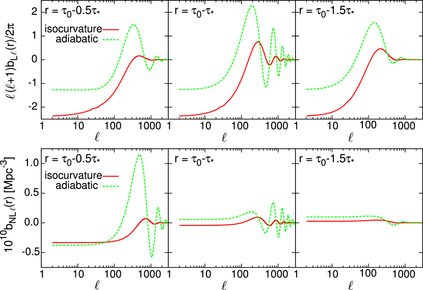
In Fig. 1 we show the numerical results of and . If we take largely different from , which is the comoving distance from us at to the last scattering surface at , both and get suppressed. This is because and in the integrant of Eqs. (44-45) would oscillate with different frequencies, making contributions in a destructive way. Therefore the signature of the primordial non-Gaussianity mostly comes from . In Fig. 1 we have taken several values of around .
Let us first consider shown in the upper panels of Fig. 1. We notice that is roughly twice as large as in the amplitude at large angular scales () for any values of . This behavior is similar to the angular power spectra . It can be easily understood by noting that the Sachs-Wolfe effect leads to
| (55) |
At smaller angular scales ’s represent the acoustic oscillations. Note that the phase of oscillations are different by between the isocurvature and adiabatic perturbations. This is another similarity of with .
On the other hand, the situation with is slightly different. Athough ’s also give similar flat spectra at the large angular scales, they have some differences from . One of them is that the ratio of the amplitudes of for isocurvature and adiabatic initial conditions differs with . This is because receives more contribution from smaller scales due to the absence of in the denominator of the integrant in Eq (45), compared with . Since the perturbations in photon fluid becomes smaller at large for isocurvature perturbations, the is not as large as . This changes Eq. (54) obtained by using the approximated transfer function in the Sachs-Wolfe regime Eq. (50). We will discuss this issue below.
Among the three terms in Eq. (43), we denote the two of them by
| (56) |
In Fig. 2, we show the bispectrum and for the isocurvature and adiabatic perturbations. One can see that the amplitude of the bispectrum of the isocurvature perturbations is enhanced at large angular scales (), compared with the adiabatic perturbations. Our numerical calculations give the ratio at large scales as
| (57) |
If the transfer function in Eq. (50) were valid at smaller scales beyond the Sachs-Wolfe plateau, the right hand side of Eq (57) would be , as expected from Eqs. (49) and (55). However as have mentioned above, receives contributions from smalle scales () in a destructive way, and this roughly halves the the amplitude of the bispectrum from isocurvature perturbations compared to that from adiabatic perturbations. At acoustic region (), the amplitude of becomes much suppressed since CMB temperature anisotropies are small at acoustic region for isocurvature initial perturbations.
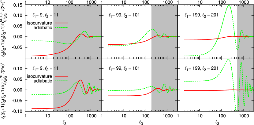
In Fig. 3 we plot as a function of for various sets of . We can see that our estimate of at large angular scales in Eq. (54) is corrected and approximately given by
| (58) |
However the amplitude of the bispectrum at large angular scales is still enhanced for non-Gaussian isocurvature perturbations compared with adiabatic perturbations. In the adiabatic case, the largest signals of the primordial non-Gaussianity come from the acoustic regions. On the other hand, in the isocurvature case, the signals are concentrated in the large angular scales. This remarkable difference in -dependence of and will help us distinguish the isocurvature non-Gaussianity from the adiabatic one.
So far, we have assumed SCDM universe. Here we give some comments on how the above results will change in the standard CDM universe. Assuming the flat universe, the amount of CDM is smaller ( [1]) in the CDM universe. For the adiabatic initial perturbations, this does not cause much difference on the CMB anisotropies at large angular scales, except for the small late-time Integrated Sachs-Wolfe effect from nonzero . On the other hand, for the isocurvature initial perturbations, the anisotropies at large angular scales will be suppressed. This is because the universe is not completely matter-dominated at recombination and therefore the curvature perturbations on large scales are not entirely generated from isocurvature perturbations in CDM (Eq. (30) is not a very good approximation in the CDM model). At large angular scales, the CMB anisotropies with the isocurvature initial perturbations are, however, still larger than for adiabatic ones and our discussion above is basically valid even in the CDM universe. When constraining the isocurvature non-Gaussianity by using the future CMB data, we should take more realistic CDM model, but there will be no fundamental difference.
4 Application to the axion
In this section we apply our formulation to the axion as a concrete example. The axion, , is a pseudo Nambu-Goldstone boson associated with the spontaneous breaking of the PQ symmetry. Let us denote the breaking scale by , whose magnitude is constrained from various experiments, astrophysical and cosmological considerations. The most strict lower bound on comes from the observation that the duration of the neutrino burst in SN1987A lasted for 10 seconds. In order to prevent too fast cooling by the axion emission, GeV is required [35]. On the other hand, the upper bound is provided by the cosmological argument. The axion obtains a tiny mass after the QCD phase transition due to the anomaly effect which explicitly breaks the PQ symmetry. The axion begins to oscillate coherently after that. Since the lifetime of the axion is very long, it survives until now and contributes to DM of the universe. The abundance is estimated as [36]
| (59) |
where denotes the initial misalignment angle of the axion. Imposing [1], we obtain an upper bound on the PQ scale as GeV. Thus the ratio of the axion abundance to the total dark matter abundance is calculated as
| (60) |
where we have defined
| (61) |
If the PQ symmetry is already broken before or during inflation and if it is never restored after inflation, the axion has unsuppressed quantum fluctuations during inflation because it remains practically massless during inflation. Since the axion contributes to some fraction of DM, such an axionic isocurvature fluctuation is converted to the CDM isocurvature fluctuation. Thus the axion is a plausible candidate for generating the non-Gaussianity from the isocurvature perturbation.
Now let us estimate the magnitude of the axionic isocurvature fluctuation and the resultant non-Gaussianity. We assume that the inflaton itself does not generate non-Gaussianity, and that only the axion has an isocurvature fluctuation. The axion acquires a quantum fluctuation during inflation given by
| (62) |
The observationally relevant quantity is the CDM isocurvature perturbation, rather than the axionic isocurvature perturbation itself. Using Eq. (9), the CDM isocurvature perturbation is given by
| (63) |
where denotes the dark matter abundance other than the axion. In this equation, is evaluated on the uniform density slicing. Since is conserved quantity as long as the scales of interest are sufficiently large, we can evaluate it when the axion starts to oscillate. When the axion starts to oscillate, the universe is dominated by the radiation, and therefore we can safely neglect the density fluctuation of the radiation, .
As will become clear later, if one imposes the current constraint on the isocurvature perturbation, large non-Gaussianity is generated only for . Using , we can approximate as
| (64) |
where denotes the classical deviation from the potential minimum. The first term in (61) dominates over the second one when the classical deviation from the potential minimum overcomes the amplitude of the quantum fluctuation. In the opposite case, i.e., the isocurvature fluctuation is dominated by the second term in (64), the whole dynamics of the axion is controlled by the quantum fluctuation generated during inflation. This is similar to the “ungaussiton” scenario [17]: the axion is predominantly produced by the quantum fluctuations, giving the non-Gaussianity to the density fluctuations, while its contribution to the total curvature perturbation is negligibly small.
For later convenience, the power spectrum of the isocurvature perturbation is defined through Eq. (17),
| (65) |
Also note that the isocurvature perturbation is uncorrelated with the primordial curvature perturbation in the case of the axion,
| (66) |
It is straitforward to calculate the non-linearity parameter defined by Eq. (26). First note that from Eqs. (24) and (25) is calculated as
| (67) |
where is the WMAP normalization of the curvature perturbation. Then Eq. (33) tells us that the non-linearity parameter is given by
| (68) |
if the classical deviation overcomes the quantum fluctuation . Since the WMAP five-year results give a contraint , a small value of is necessary for large non-Gaussianity, . But there is an upper bound on the level of non-Gaussianity coming from CDM isocurvature perturbation. In order to maximize the value of , the isocurvature perturbation must also be large. However, since is limited as , is maximized at in order to saturate the isocurvature bound and this gives a strict upper bound as . This is explicitly shown in the case , where the quantum fluctuation dominates the axion dynamics, giving . In this case the non-linearlity parameter is estimated as
| (69) |
Note that in this regime the parameter dependence of is all compressed in the information of the magnitude of the isocurvature perturbation. Thus non-Gaussianity parameter is solely bounded by the isocurvature constraint in this regime. In other words, is maximized when the isocurvature contribution saturates the allowed maximum value and the bound does not depend on other model parameters. It may also be useful to give a full expression for ,
| (70) |
whose limiting behavior approaches to the expressions given above.
Above results can be understood in a simple way. The following rough estimations may be useful because they give a correct parameter dependence. When the isocurvature perturbation is dominantly given by the linear Gaussian part , and hence the three point function is estimated as . Thus we obtain
| (71) |
On the other hand when , The non-Gaussian part dominates the isocurvature perturbation , giving a three point function as . As a result we obtain
| (72) |
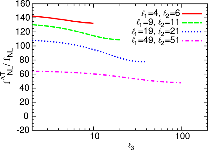
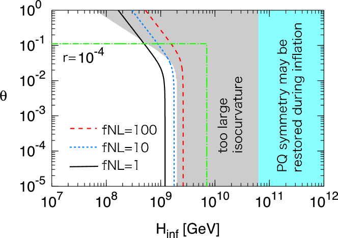
In Figs. 4, 5 and 6, the non-linearlity parameter is shown on - plane for GeV, GeV, and GeV. It is seen that an observable amount of non-Gaussianity (say, ) is generated near the isocurvature constraint. However, notice that the relevant quantity from CMB observations is , not , and the relation between them is given in Sec. 3. In particular it has been shown that can be times larger than , depending on the observed scale. Thus it may be possible that isocurvature fluctuation is probed only through its non-Gaussian imprints on CMB.


5 Conclusions and Discussion
In this paper we have investigated a possibility that large non-Gaussianity is generated by isocurvature fluctuations. One interesting feature of this scenario is that the bispectrum and the power spectrum of the CMB temperature fluctuations exhibit characteristic scale dependence. In particular, the effective non-linearity parameter is significantly enhanced at large scales, compared to the adiabatic case. Furthermore, our results indicate that large non-Gaussianity may be accompanied with an observable fraction of the isocurvature perturbation. If future observations confirm both large non-Gaussianity and a certain amount of isocurvature fluctuation component, our scenario will become very attractive. As a concrete example, we have shown that the axion can naturally induce such isocurvature perturbation in the CDM sector, leading to large non-Gaussianity. If the axion is indeed responsible for the large non-Gaussianity hinted by the current observations, the inflationary scale should be in the range of GeV. This opens up an interesting possibility that the axion can be probed through its non-Gaussianity contribution to the CMB temperature fluctuation, even if the energy density of the axion today is negligible compared to the total dark matter abundance 555 There may be an anthropic reason that forces the axion abundance to take such value [37]. .
Although we have restricted ourselves to the CDM isocurvature perturbation in this paper, the baryonic isocurvature perturbation can also generate large non-Gaussianity in a similar fashion [38]. There is indeed a scenario using the flat direction with the baryon number to generate baryonic isocurvature perturbations [39, 40, 41].
We have assumed that the CDM isocurvature perturbation comes from the fluctuations in the CDM sector. However, this may not be the case, and it can arise from the radiation. That is to say, the CDM isocurvature perturbation is given by in some cases, including the curvaton/ungaussiton scenario. In this case the sign of the non-linearity parameter becomes negative, which is expected to leave distinct features on the bispectrum of the temperature fluctuation. One may be able to use the features to probe into the origin of the isocurvature perturbation [42].
In general, the isocurvature perturbation mainly affects the large scale temperature anisotropy, while its effect on the density perturbation is weaker than the adiabatic one. Thus if the non-Gaussianity is truly sourced by the isocurvature perturbation, it can be seen only in the CMB observations, and we should have null detection of non-Gaussianity from the analyses using the matter power spectra. Hopefully, future cosmological observations will enable us to establish or refute the existence of large non-Gaussianity. If it is there, we may be able to distinguish the origin, adiabatic or isocurvature. Undoubtedly, once detected, it will provide us with useful information on the early universe and the high energy physics.
Acknowledgment
K. Nakayama and T. Sekiguchi would like to thank the Japan Society for the Promotion of Science for financial support. This work is supported by Grant-in-Aid for Scientific research from the Ministry of Education, Science, Sports, and Culture (MEXT), Japan, No.14102004 (M.K.) and also by World Premier International Research Center Initiative (WPI Initiative), MEXT, Japan.
References
- [1] E. Komatsu et al. [WMAP Collaboration], arXiv:0803.0547 [astro-ph].
- [2] R. Bean, J. Dunkley and E. Pierpaoli, Phys. Rev. D 74, 063503 (2006) [arXiv:astro-ph/0606685]; R. Trotta, Mon. Not. Roy. Astron. Soc. Lett. 375, L26 (2007) [arXiv:astro-ph/0608116]; R. Keskitalo, H. Kurki-Suonio, V. Muhonen and J. Valiviita, JCAP 0709, 008 (2007) [arXiv:astro-ph/0611917]; M. Kawasaki and T. Sekiguchi, arXiv:0705.2853 [astro-ph]; M. Beltran, J. Garcia-Bellido and J. Lesgourgues, Phys. Rev. D 75, 103507 (2007) [arXiv:hep-ph/0606107].
- [3] A. P. S. Yadav and B. D. Wandelt, arXiv:0712.1148 [astro-ph].
- [4] A. Slosar, C. Hirata, U. Seljak, S. Ho and N. Padmanabhan, arXiv:0805.3580 [astro-ph]; N. Afshordi and A. J. Tolley, arXiv:0806.1046 [astro-ph]; P. McDonald, arXiv:0806.1061 [astro-ph]; C. Carbone, L. Verde and S. Matarrese, arXiv:0806.1950 [astro-ph]; A. Bernui and M. J. Reboucas, arXiv:0806.3758 [astro-ph]; U. Seljak, arXiv:0807.1770 [astro-ph].
- [5] R. D. Peccei and H. R. Quinn, Phys. Rev. Lett. 38, 1440 (1977).
- [6] For reviews, see J. E. Kim, Phys. Rept. 150, 1 (1987); J. E. Kim and G. Carosi, arXiv:0807.3125 [hep-ph].
- [7] J. Preskill, M. B. Wise and F. Wilczek, Phys. Lett. B 120, 127 (1983); L. F. Abbott and P. Sikivie, Phys. Lett. B 120, 133 (1983); M. Dine and W. Fischler, Phys. Lett. B 120, 137 (1983).
- [8] D. Seckel and M. S. Turner, Phys. Rev. D 32, 3178 (1985); M. S. Turner and F. Wilczek, Phys. Rev. Lett. 66, 5 (1991).
- [9] A. D. Linde, Phys. Lett. B 259, 38 (1991).
- [10] V. Acquaviva, N. Bartolo, S. Matarrese and A. Riotto, Nucl. Phys. B 667, 119 (2003) [arXiv:astro-ph/0209156].
- [11] J. M. Maldacena, JHEP 0305, 013 (2003) [arXiv:astro-ph/0210603].
- [12] D. Seery and J. E. Lidsey, JCAP 0506, 003 (2005) [arXiv:astro-ph/0503692]; D. Seery and J. E. Lidsey, JCAP 0509, 011 (2005) [arXiv:astro-ph/0506056]; D. Seery, J. E. Lidsey and M. S. Sloth, JCAP 0701, 027 (2007) [arXiv:astro-ph/0610210].
- [13] S. Yokoyama, T. Suyama and T. Tanaka, Phys. Rev. D 77, 083511 (2008) [arXiv:0705.3178 [astro-ph]].
- [14] S. Mollerach, Phys. Rev. D 42, 313 (1990).
- [15] A. D. Linde and V. F. Mukhanov, Phys. Rev. D 56, 535 (1997) [arXiv:astro-ph/9610219]; JCAP 0604, 009 (2006) [arXiv:astro-ph/0511736].
- [16] D. H. Lyth and D. Wands, Phys. Lett. B 524, 5 (2002) [arXiv:hep-ph/0110002]; T. Moroi and T. Takahashi, Phys. Lett. B 522, 215 (2001) [Erratum-ibid. B 539, 303 (2002)] [arXiv:hep-ph/0110096]; K. Enqvist and M. S. Sloth, Nucl. Phys. B 626, 395 (2002) [arXiv:hep-ph/0109214].
- [17] T. Suyama and F. Takahashi, JCAP 0809, 007 (2008) [arXiv:0804.0425 [astro-ph]].
- [18] D. H. Lyth, C. Ungarelli and D. Wands, Phys. Rev. D 67, 023503 (2003) [arXiv:astro-ph/0208055].
- [19] N. Bartolo, S. Matarrese and A. Riotto, Phys. Rev. D 69, 043503 (2004) [arXiv:hep-ph/0309033].
- [20] D. H. Lyth and Y. Rodriguez, Phys. Rev. Lett. 95, 121302 (2005) [arXiv:astro-ph/0504045].
- [21] D. H. Lyth, JCAP 0606, 015 (2006) [arXiv:astro-ph/0602285].
- [22] K. A. Malik and D. H. Lyth, JCAP 0609, 008 (2006) [arXiv:astro-ph/0604387].
- [23] K. Ichikawa, T. Suyama, T. Takahashi and M. Yamaguchi, arXiv:0802.4138 [astro-ph].
- [24] M. Beltran, arXiv:0804.1097 [astro-ph].
- [25] N. Bartolo, S. Matarrese and A. Riotto, Phys. Rev. D 65, 103505 (2002) [arXiv:hep-ph/0112261].
- [26] L. Boubekeur and D. H. Lyth, Phys. Rev. D 73, 021301 (2006) [arXiv:astro-ph/0504046].
- [27] D. H. Lyth, K. A. Malik and M. Sasaki, JCAP 0505, 004 (2005) [arXiv:astro-ph/0411220].
- [28] D. Wands, K. A. Malik, D. H. Lyth and A. R. Liddle, Phys. Rev. D 62, 043527 (2000) [arXiv:astro-ph/0003278].
- [29] D. H. Lyth, Phys. Rev. D 45, 3394 (1992).
- [30] D. H. Lyth, JCAP 0712, 016 (2007) [arXiv:0707.0361 [astro-ph]].
- [31] N. Bartolo, E. Komatsu, S. Matarrese and A. Riotto, Phys. Rept. 402, 103 (2004) [arXiv:astro-ph/0406398].
- [32] E. Komatsu and D. N. Spergel, Phys. Rev. D 63, 063002 (2001) [arXiv:astro-ph/0005036].
- [33] E. Komatsu, D. N. Spergel and B. D. Wandelt, Astrophys. J. 634, 14 (2005) [arXiv:astro-ph/0305189].
- [34] A. Lewis, A. Challinor and A. Lasenby, Astrophys. J. 538, 473 (2000) [arXiv:astro-ph/9911177].
- [35] G. G. Raffelt, Phys. Rept. 198, 1 (1990).
- [36] M. S. Turner, Phys. Rev. D 33, 889 (1986).
- [37] K. Nakayama and F. Takahashi, to appear.
- [38] M. Kawasaki, K. Nakayama and F. Takahashi, arXiv:0809.2242 [hep-ph].
- [39] K. Enqvist and J. McDonald, Phys. Rev. Lett. 83, 2510 (1999); Phys. Rev. D 62, 043502 (2000).
- [40] M. Kawasaki and F. Takahashi, Phys. Lett. B 516, 388 (2001).
- [41] S. Kasuya, M. Kawasaki and F. Takahashi, arXiv:0805.4245 [hep-ph].
- [42] M. Kawasaki, K. Nakayama, T. Sekiguchi, T. Suyama and F. Takahashi, arXiv:0810.0208 [astro-ph].