Coexistence of ordered and disordered phases in Potts models in the continuum

Abstract.

This is the second of two papers on a continuum version of the Potts model, where particles are points in $\mathbb{R}^{d}$, $d\geq 2$, with a spin which may take $S\geq 3$ possible values. Particles with different spins repel each other via a Kac pair potential of range $\gamma^{-1}$, $\gamma>0$. In this paper we prove phase transition, namely we prove that if the scaling parameter of the Kac potential is suitably small, given any temperature there is a value of the chemical potential such that at the given temperature and chemical potential there exist $S+1$ mutually distinct DLR measures.

1. Introduction

The conjecture that mean field phase diagrams are well approximated by systems with long range interactions cannot be taken literally as it obviously fails in one dimensional systems (if the second moment of the interaction is finite), moreover the mean field critical exponents are [believed to be] different from those computed for finite range interactions. With proper caveat however the conjecture is generally regarded as correct and indeed there are mathematical proofs mainly referring to specific models and focused on the occurrence of phase transitions. The choice of the approximating hamiltonian is not at all arbitrary and the results so far have been obtained for reflection positive interactions, [6], and for Kac potentials, [5]. The former choice is clearly motivated by a powerful and well developed theory, the latter class seems more general, in particular includes systems of particles in the continuum as the one considered in the present paper. We will in fact study here a continuum version of the classical Potts model. Its mean field free energy is

$$F^{\rm mf}_{\beta,\lambda}(\rho)=\frac{1}{2}\sum_{s\neq s^{\prime}}\rho_{s}\rho_{s^{\prime}}-\lambda\sum_{s}\rho_{s}-\frac{1}{\beta}\mathcal{S}(\rho),\qquad\mathcal{S}(\rho)=-\sum_{s}\rho_{s}[\log\rho_{s}-1]$$ (1.1)

$\rho=\{\rho_{1},..,\rho_{S}\}\in\mathbb{R}_{+}^{S}$, $\rho_{s}$ represents the density of particles with spin $s$, $s\in\{1,..,S\}$, $S\geq 3$; $\beta$ the inverse temperature; $\lambda$ the chemical potential.

Despite the simplicity of the model its thermodynamics, which is defined by minimizing $F^{\rm mf}_{\beta,\lambda}(\rho)$ over $\rho\in\mathbb{R}_{+}^{S}$, has a rather interesting structure. In [10] and [7] it is proved that the resulting phase diagram is characterized by a critical curve $\lambda=\lambda_{\beta},\beta>0$, as in Figure 1.

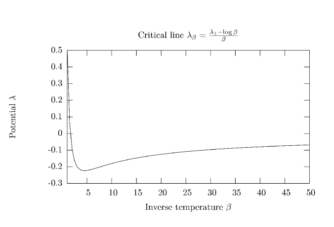
Figure 1. Phase Diagram of the Mean field Potts gas

$F^{\rm mf}_{\beta,\lambda_{\beta}}$ has $S+1$ minimizers $\rho^{(k)}=(\rho_{s}^{(k)},s=1,..,S)$, $k=1,..,S+1$. There are positive numbers $a$, $b<c$ so that

$$\rho^{(S+1)}_{s}=a,\,\,\,\forall s,\qquad\text{ for }k\leq S:\;\;\rho^{(k)}_{s}=b\,\,\,\forall s\neq k,\,\,\,\quad\rho^{(k)}_{k}=c$$ (1.2)

Furthermore

$$Sa<b^{*},\quad b^{*}:=(S-1)b+c$$ (1.3)

so that the total density of the state $\rho^{(S+1)}$ is smaller than the total density in any of the ordered critical points $\rho^{(k)}$, $k\leq S$, which is in fact equal to $b^{*}$.

When $\lambda>\lambda_{\beta}$, only the ordered states survive and there are $S$ minimizers, when $\lambda<\lambda_{\beta}$, only the disordered state survives and there is a unique minimizer. Therefore when crossing vertically the critical curve the total density jumps, a phenomenon which can be related to magnetostriction as argued in [7].

The Kac proposal applied to (1.1) leads to hamiltonians of the form

$$H_{\gamma,\lambda}(q)=\frac{1}{2}\sum_{i\neq j}V_{\gamma}(r_{i},r_{j})\text{\bf 1}_{s_{i}\neq s_{j}}-\lambda n$$ (1.4)

where $q=(...,r_{i},s_{i},...)$, $i=1,..,n$, $r_{i}\in\mathbb{R}^{d}$, $s_{i}\in\{1,..,S\}$, is a finite configuration of particles with spin; $\lambda$ the chemical potential and $V_{\gamma}(r_{i},r_{j})=\gamma^{d}V(\gamma r_{i},\gamma r_{j})$, $V(r,r^{\prime})$ a symmetric probability kernel, say with range 1. An analysis a la Lebowitz and Penrose, [14] (see also Gates and Penrose, [9]) proves that the mesoscopic ($\gamma\to 0$) behavior of the system with hamiltonian $H_{\gamma,\lambda}(q)$ is described by

$$F_{\beta,\lambda}(\rho)=\frac{1}{2}\sum_{s,s^{\prime}:s\neq s^{\prime}}\int\rho_{s}(r)V(r,r^{\prime})\rho_{s^{\prime}}(r^{\prime})drdr^{\prime}-\int\{\frac{\mathcal{S}(\rho(r))}{\beta}+\lambda\sum_{s}\rho_{s}(r)\}dr$$ (1.5)

as a functional defined on functions $\rho\in L^{\infty}(\mathbb{R}^{d},\mathbb{R}_{+}^{S})$ with compact support. Let $\Lambda$ a torus in $\mathbb{R}^{d}$, call $F_{\beta,\lambda,\Lambda}(\rho)$ the functional (1.5) on $L^{\infty}(\Lambda,\mathbb{R}_{+}^{S})$, then obviously

$$\inf_{\rho\in L^{\infty}(\Lambda,\mathbb{R}_{+}^{S})}F_{\beta,\lambda,\Lambda}(\rho)\leq|\Lambda|\inf_{\rho\in\mathbb{R}_{+}^{S}}F^{\rm mf}_{\beta,\lambda}(\rho)$$ (1.6)

(just restrict the inf on the l.h.s. to constant functions). Thus a preliminary condition for the particle model to have mean field behavior is to require that (1.6) holds with equality, which (we suspect) requires extra conditions on $V$.

In [15] the Kac proposal has been modified in such a way that the above condition is automatically satisfied. Call $e^{\rm mf}_{\lambda}(\rho)$ the mean field energy, in our case

$$e^{\rm mf}_{\lambda}(\rho)=\frac{1}{2}\sum_{s,s^{\prime}:s\neq s^{\prime}}\rho_{s}\rho_{s^{\prime}}-\lambda\sum_{s}\rho_{s}$$ (1.7)

(i.e. the first two terms on the r.h.s. of (1.1), the third one is the contribution of the entropy to the free energy) and set

$$H_{\gamma,\lambda}(q)=\int e^{\rm mf}_{\lambda}(J_{\gamma}*q(r))\,dr,\;\;\;\text{$J_{\gamma}*q(r)\in\mathbb{R}_{+}^{S}$, $\displaystyle{(J_{\gamma}*q)(r,s)=\sum_{i}J_{\gamma}(r,r_{i})\text{\bf 1}_{s_{i}=s}}$}$$ (1.8)

$J_{\gamma}(r,r^{\prime})=\gamma^{d}J(\gamma r,\gamma r^{\prime})$ with $J(r,r^{\prime})$ a smooth, symmetric, translational invariant probability kernel with range 1, $J(r,r^{\prime})=0$ if $|r-r^{\prime}|\geq 1$.

Namely the “modified Kac proposal” we are adopting is to suppose that the particle hamiltonian has an energy density at point $r$ given by the mean field free energy computed on the empirical density $J_{\gamma}*q(r)$. Analogous prescription can be applied whenever the mean field order parameter is a density (or as in this case a collection of densities). The free energy functional associated to (1.8) is, supposing $\Lambda$ a torus in $\mathbb{R}^{d}$,

$$F_{\beta,\lambda,\Lambda}(\rho)=\int_{\Lambda}\{e^{\rm mf}_{\lambda}(J*\rho(r))-\frac{\mathcal{S}(\rho(r))}{\beta}\}$$ (1.9)

which can be rewritten as

$$F_{\beta,\lambda,\Lambda}(\rho)=\int_{\Lambda}\{e^{\rm mf}_{\lambda}(J*\rho(r))-\frac{\mathcal{S}(J*\rho(r))}{\beta}\}+\frac{1}{\beta}\int_{\Lambda}\{\mathcal{S}(J*\rho)-J*\mathcal{S}(\rho)\}$$ (1.10)

By convexity the second integral is non negative and 0 on the constants; the first one is minimized by taking $\rho(r)$ constantly equal to the minimizer of $F^{\rm mf}_{\beta,\lambda}(\cdot)$. Thus (1.6) holds in this case with equality.

Notice that the hamiltonian $H_{\gamma,\lambda}(q)$ of (1.8) has the form (1.4) because it can be written as

$$H_{\gamma,\lambda}(q)=\frac{1}{2}\sum_{i\neq j}(J_{\gamma}*J_{\gamma})(r_{i},r_{j})\text{\bf 1}_{s_{i}\neq s_{j}}-\lambda n$$ (1.11)

Thus the LMP prescription in this case is just a positivity assumption on the kernel $V$ (more precisely $V=J_{\gamma}*J_{\gamma}$). In the sequel we will restrict to the choice (1.8)–(1.11). The main result in this paper is

Theorem 1.1.

For any $d\geq 2$, $S\geq 3$, $\beta>0$ there is $\gamma^{*}>0$ and for any $\gamma\leq\gamma^{*}$ there are $\lambda_{\beta,\gamma}$ and $S+1$ DLR measures at $(\beta,\lambda_{\beta,\gamma})$, denoted by $\mu^{(k)},k\in\{1,\dots,S+1\}$, with the following properties.

$\bullet$  Each $\mu^{(k)}$ is a translational invariant, extremal DLR measure (with trivial $\sigma$-algebra at infinity);

$\bullet$  any translational invariant DLR measure is a convex combination of $\big{\{}\mu^{(k)},k\in\{1,..,S+1\}\big{\}}$;

$\bullet$  calling $\rho_{\gamma,s^{\prime}}^{(k)},s^{\prime}\in\{1,..,S\}$ the average density of particles with spin $s^{\prime}$ in $\mu^{(k)}$ and $\rho^{(k)}_{s}$ the mean field values, $\displaystyle{\lim_{\gamma\to 0}\rho_{\gamma,s^{\prime}}^{(k)}=\rho^{(k)}_{s^{\prime}}}$;

$\bullet$  any measure $\mu^{(k)}$, $k\leq S$, is invariant under any exchange of spin labels which does not involve $k$ while $\mu^{(S+1)}$ is invariant under any exchange of spin labels.

The proof of Theorem 1.1 uses specific features of the model besides the property that (1.6) is true with equality. Which properties are of general nature and which ones are instead truly specific of the model is difficult to say. To a great extent the proof follows from the analysis (a la Pirogov-Sinai) of the LMP model in Chapter 11 and 12 of [16], but there are several points where we need to overcome important difficulties not present in the LMP model. Among them the main one is about the exponential decay of correlations in the restricted ensemble, Theorem 3.1 of the companion paper [7]. How to go from such a result to the proof of Theorem 1.1 is the content of the present paper.

Theorem 1.1 does not claim anything away from $(\beta,\lambda_{\beta,\gamma})$, this allows to simplify the traditional Pirogov-Sinai approach. The conjecture is that when $\lambda$ varies in $(\lambda_{\beta,\gamma}-\epsilon,\lambda_{\beta,\gamma}+\epsilon)$, $\epsilon>0$ suitably small, then we go from uniqueness $\lambda<\lambda_{\beta,\gamma}$ to $S$ extremal states, $\lambda>\lambda_{\beta,\gamma}$, (always referring to translational invariant DLR states). The Potts model does not exactly fall in the class considered in [3] but presumably the analysis in [3] can be extended to prove the above conjecture. It is also plausible that the estimates are uniform in a small neighborhood of $\beta$, in such a case we would have local closeness of the mean field and the finite $\gamma$ phase diagrams, thus partially confirming the validity of the conjecture in the beginning of the introduction.

In Part I we define the model and establish the main notation, Section 2, and then prove Theorem 1.1, Section 3, supposing that the Peierls estimates on contours are valid. In Part II we prove the Peierls estimates, this being the more technical part of the paper.

Part I

2. Main notation and definitions

We start with the basic definitions. They are quite standard and consistent with those of the companion paper [7].

2.1. Geometrical notions

We give the following definitions.

$\bullet$  The partitions $\mathcal{D}^{(\ell)}$.

We denote by $\mathcal{D}^{(\ell)}$, $\ell>0$, the partition $\{C^{(\ell)}_{x},\,x\in\ell\mathbb{Z}^{d}\}$ of $\mathbb{R}^{d}$ into the cubes $C^{(\ell)}_{x}=\{r\in\mathbb{R}^{d}:x_{i}\leq r_{i}<x_{i}+\ell,i=1,..,d\}$ ($r_{i}$ and $x_{i}$ the cartesian components of $r$ and $x$). We call $C^{(\ell)}_{r}$ the cube which contains $r\in\mathbb{R}^{d}$.

$\bullet$  $\mathcal{D}^{(\ell)}$-measurable sets and functions.

A set is $\mathcal{D}^{(\ell)}$-measurable if it is union of cubes in $\mathcal{D}^{(\ell)}$. A function $f:\mathbb{R}^{d}\times\{1,\dots,S\}\to\mathbb{R}$ is $\mathcal{D}^{(\ell)}$-measurable if its inverse images are $\mathcal{D}^{(\ell)}$-measurable sets, or, equivalently, if it is constant on the cubes of $\mathcal{D}^{(\ell)}$.

$\bullet$  $\mathcal{D}^{(\ell)}$-boundaries of a set.

Calling two sets connected if their closures have non empty intersection, given a $\mathcal{D}^{(\ell)}$-measurable region $\Lambda$ we call $\delta_{\rm out}^{\ell}[\Lambda]$ the union of all cubes of $\mathcal{D}^{(\ell)}$ in $\Lambda^{c}\equiv\mathbb{R}^{d}\setminus\Lambda$ which are connected to $\Lambda$. Analogously we call $\delta_{\rm in}^{\ell}[\Lambda]$ the union of all cubes of $\mathcal{D}^{(\ell)}$ in $\Lambda$ which are connected to $\Lambda^{c}$.

2.2. Phase space, topology and free measure

We start with the definition of the phase space.

$\bullet$  The phase space $\mathcal{Q}$.

It is convenient to represent the phase space $\mathcal{Q}$ of the Potts model as a spin system on the lattice, the spins taking values in a non compact space. With $\{C_{i}\equiv C_{i}^{(1)},i\in\mathbb{Z}^{d}\}$ the cubes of the partition $\mathcal{D}^{(1)}$, we then define $\displaystyle{\mathcal{Q}_{C_{i}}:=\bigcup_{n\geq 0}(C_{i}\times\{1,\dots,S\})^{n}}$ and $\mathcal{Q}=\prod_{i}\mathcal{Q}_{C_{i}}$.

Thus an element $q\in\mathcal{Q}$ is a sequence $q^{(i)}\in\mathcal{Q}_{C_{i}}$, if $q^{(i)}=(r_{1},s_{1},\dots,r_{n},s_{n})$ we will then say that in $C_{i}$ there are $n$ particles at positions $r_{j}$ with spins $s_{j}$, $j=1,..,n$. As particles are undistinguishable, physical observables are functions symmetric under exchange of particles labels and the actual physical phase space is $\mathcal{Q}^{\rm sym}=\prod_{i}\mathcal{Q}_{C_{i}}^{\rm sym}$ which is obtained by taking the quotient under permutation of indices. To simplify notation in the sequel we will just write $\mathcal{Q}$ being clear from the context if we are referring to $\mathcal{Q}^{\rm sym}$. Since labels are unimportant we can write a configuration $q\in\mathcal{Q}$ as a sequence $q=\{...,r_{j},s_{j},...\}$, $r_{j}\in\mathbb{R}^{d}$, $s_{j}\in\{1,..,S\}$, indeed $q_{C_{i}}=q\cap C_{i}$, namely the set of all $(r_{j},s_{j})\in q:r_{j}\in C_{i}$, identifies the component of $q$ in $\mathcal{Q}_{C_{i}}$. Given $q=\{...,r_{j},s_{j},...\}\in\mathcal{Q}$ we write $q(s)=\{(r_{j},s_{j})\in q:s_{j}=s\}$ and we call $\mathcal{Q}_{\Lambda}:=\{q_{\Lambda}\in\mathcal{Q}:q_{\Lambda}=\{(r_{j},s_{j})\in q:r_{j}\in\Lambda\}\}$. We finally denote by $q\cup q^{\prime}$ the configuration which collects all the particles in $q$ and $q^{\prime}$, evidently referring here to indistinguishable particle configurations.

$\bullet$  Topological properties of $\mathcal{Q}$.

We consider $\displaystyle{\mathcal{Q}_{C_{i}}=\bigcup_{n\geq 0}(C_{i}\times\{1,\dots,S\})^{n}}$ equipped with its natural topology and $\mathcal{Q}$ with the product topology calling $\Sigma$ the corresponding Borel $\sigma$-algebra.

While the product topology in $\mathcal{Q}$ is not physically correct (the path of a particle moving continuously from a cube $C_{i}$ to another one is not continuous in the product topology) yet the Borel structure is not changed and since we are interested in measure theoretically properties the above definition becomes acceptable.

$\bullet$  The free measure.

We denote by $\nu(dq_{C_{i}})$ the measure on $\mathcal{Q}_{C_{i}}$ which restricted to $(C_{i}\times\{1,.,S\})^{n}$ is equal to $(n!)^{-1}dr_{1}..dr_{n}$, such that if $f$ is a bounded measurable function on $\mathcal{Q}_{C_{i}}$

$$\int_{\mathcal{Q}_{C_{i}}}f(q)\nu(dq_{C_{i}})=\sum_{n=0}^{\infty}\frac{1}{n!}\sum_{s_{1},\dots,s_{n}}\int_{C_{i}^{n}}f(r_{1},s_{1},\dots,r_{n},s_{n})dr_{1}\dots dr_{n}$$

If $\Lambda$ is a bounded $\mathcal{D}^{(1)}$ measurable region we define the free measure $\displaystyle{\nu(dq_{\Lambda})=\prod_{i\in\Lambda\cap\mathbb{Z}^{d}}\nu(dq_{C_{i}})}$ on $\mathcal{Q}_{\Lambda}$ observing that for any measurable set $\Delta\subseteq\Lambda$

$$\int_{\mathcal{Q}_{\Delta}}f(q)\nu(dq_{\Lambda})=\sum_{n=0}^{\infty}\frac{1}{n!}\sum_{s_{1},\dots,s_{n}}\int_{\Delta^{n}}f_{n}(r_{1},s_{1},\dots,r_{n},s_{n})dr_{1}\dots dr_{n}$$ (2.1)

2.3. Energy and Gibbs measures

We have already defined the energy $H_{\gamma,\lambda}(q)$ (of a finite configuration), see (1.8). The energy in a bounded set $\Lambda$ with boundary condition $\bar{q}_{\Lambda^{c}}$ is defined as usual as

$$H_{\Lambda,\lambda}(q_{\Lambda}|\bar{q}_{\Lambda^{c}})=H_{\lambda}(q_{\Lambda}\cup\bar{q}_{\Lambda^{c}})-H_{\lambda}(\bar{q}_{\Lambda^{c}})=\int_{\mathbb{R}^{d}}\big{[}e_{\lambda}^{\rm mf}\big{(}J_{\gamma}\star(q_{\Lambda}\cup q_{\Lambda^{c}})\big{)}-e_{\lambda}^{\rm mf}\big{(}J_{\gamma}\star q_{\Lambda^{c}}\big{)}\big{]}dr$$ (2.2)

The expression on the r.h.s. depends only on the particles of $\bar{q}_{\Lambda^{c}}$ at distance $\leq 2\gamma^{-1}$.

In the sequel we will sometimes replace $\bar{q}_{\Lambda^{c}}$ by $\sigma$-finite measures by setting

$$J_{\gamma}\star d\mu(r,s)=\int_{\mathbb{R}^{d}}J_{\gamma}(r,r^{\prime})d\mu(r^{\prime},s)$$ (2.3)

$d\mu(r,s)$ any non negative $\sigma$-finite measure on $\mathbb{R}^{d}\times\{1,\dots,S\}$. By identifying $q\in\mathcal{Q}$ as a sum of Dirac deltas we may regard the convolution $J_{\gamma}\star q$ as a particular case of (2.3). In particular we will often consider

$$H_{\Lambda,\lambda}(q_{\Lambda}|\chi^{(k)}_{\Lambda^{c}})=\int_{\mathbb{R}^{d}}\big{[}e_{\lambda}^{\rm mf}\big{(}J_{\gamma}\star q_{\Lambda}+J_{\gamma}\star\chi^{(k)}_{\Lambda^{c}})\big{)}-e_{\lambda}^{\rm mf}\big{(}J_{\gamma}\star\chi^{(k)}_{\Lambda^{c}}\big{)}\big{]}dr$$ (2.4)

where $\chi^{(k)}_{\Lambda^{c}}:=\rho^{(k)}\mathbf{1}_{\Lambda^{c}}$ were $\rho^{(k)}=(\rho^{(k)}_{1},\dots\rho^{(k)}_{S})$, $k\in\{1,\dots,S+1\}$ is one of the minimizers of the mean field free energy $F^{\rm mf}_{\beta,\lambda_{\beta}}$.

The Gibbs measure in $\Lambda$ ($\Lambda$ a bounded, measurable set in $\mathbb{R}^{d}$) with boundary conditions $\bar{q}$ is

$$G_{\lambda,\Lambda,\bar{q}}(dq_{\Lambda})=Z^{-1}_{\Lambda,\bar{q}}e^{-\beta H_{\Lambda,\lambda}(q_{\Lambda}|\bar{q}_{\Lambda^{c}})}d\nu(q_{\Lambda})$$ (2.5)

where the partition function $Z_{\Lambda,\bar{q}}$ is the normalization factor in (2.5). We will also consider more general boundary conditions with $\bar{q}$ replaced by $\sigma$-finite measure, the formula is again (2.5) with the energy defined using (2.3).

2.4. Phase indicators and restricted phase space

As usual in statistical mechanics local equilibrium and deviations from equilibrium are defined in terms of “averages” and of “coarse grained” variables. We briefly recall the main notion adapted to the present context. Given a configuration $q\in\mathcal{Q}$ we denote by $n^{(\ell)}(r,s;q)$ the number of particles in the configuration $q$ which are in the cube $C_{r}^{(\ell)}$ and have spin $s$, namely

$$n^{(\ell)}(r,s;q):=|q(s)\cap C_{r}^{(\ell)}|,\qquad s\in\{1,\dots,S\}$$ (2.6)

We also define the density of particles in $C_{r}^{\ell}$,

$$\rho^{(\ell)}(r,s;q):=\frac{n^{(\ell)}(r,s;q)}{\ell^{d}},\qquad s\in\{1,\dots,S\}$$ (2.7)

The phase indicators are introduced using two scales $\ell_{-}$ and $\ell_{+}$ and an accuracy parameter $\zeta$. All these numbers depend on $\gamma$ and there is much flexibility about their choice, for the sake of definitiveness we fix them as follows:

Definition 2.1.

(Choice of parameters). We choose $\ell_{-}$ and $\ell_{+}$ as functions of $\gamma$:

$$\ell_{-}=\gamma^{-1+\alpha_{-}},\quad\ell_{+}=\gamma^{-1-\alpha_{+}},\qquad\alpha_{-}<1,\quad\alpha_{+}<1$$ (2.8)

supposing for simplicity that $\gamma^{-1}$ and $\gamma^{-(1\pm\alpha_{\pm})}$ are both in $\{2^{n},n\in\mathbb{N}\}$. We also choose

$$\zeta=\gamma^{a},\qquad a<1$$

We require that $\alpha_{+}>\alpha_{-}>a$ and

$$2ad+\alpha_{-}d^{2}<\frac{\alpha_{+}}{2},\qquad\frac{1}{2}-2d\alpha_{+}>0,\qquad\frac{1}{4}-d(\alpha_{+}-\alpha_{-})>0$$ (2.9)

$$\frac{\alpha_{+}+\alpha_{-}}{1-\alpha_{-}}<\frac{1}{d},\qquad 4(\alpha_{+}+\alpha_{-})+\frac{\alpha_{-}}{2}<\frac{1}{4}$$ (2.10)

Thus for $\gamma$ small, $\ell_{-}$ is much larger than 1 and much smaller than $2\gamma^{-1}$ equal to the range of the interaction; it defines a scale large enough to make statistics reliable. Indeed, the scale $\ell_{-}$ is used together with the accuracy parameter $\zeta$ to determine if a configuration (or a density) is close to a mean field equilibrium value in a cube $C^{(\ell_{-})}$. This will be done via the phase indicator that we denote by $\eta$. Local equilibrium is instead present when the above closeness extends to regions in the scale $\ell_{+}$ thus regions with a diameter much larger than the interaction range. To quantify the local equilibrium we use the phase indicator on the scale $\ell_{+}$ that we denote by $\Theta$.

For any $\rho\in L^{1}(\mathbb{R}^{d}\times\{1,\dots,S\})$ we then define in analogy to (2.7)

$$\rho^{(\ell)}(r,s)={\displaystyle{\int\kern-12.23447pt-}}_{\kern-5.97527pt\begin{subarray}{c}C^{(\ell_{-})}_{r}\end{subarray}}\;\;\rho(x,s)dx,\qquad{\displaystyle{\int\kern-12.23447pt-}}_{\kern-5.97527pt\begin{subarray}{c}A\end{subarray}}\;\;:=\frac{1}{|A|}\int_{A}$$

and

$$\eta^{(\zeta,\ell_{-})}(r;\rho)=\begin{cases}k&\text{if $|\rho^{(\ell)}(r,s)-\rho^{(k)}_{s}|\leq\zeta$},\forall s\\ 0&\text{otherwise}\end{cases}$$ (2.11)

and

$$\Theta^{(\zeta,\ell_{-},\ell_{+})}(r;\rho)=\begin{cases}k&\text{if $\eta^{(\zeta,\ell_{-})}(\cdot;\rho)=k$ in $C^{(\ell_{+})}_{r}\cup\delta_{\rm out}^{\ell_{+}}[C^{(\ell_{+})}_{r}],$}\\ 0&{\rm otherwise}.\end{cases}$$ (2.12)

Recalling (2.7), the previous definitions extend to particle configurations $q$ by setting

$$\eta^{(\zeta,\ell_{-})}(r;q)=\eta^{(\zeta,\ell_{-})}(r;\rho^{(\ell_{-})}(q;\cdot)),\qquad\Theta^{(\zeta,\ell_{-},\ell_{+})}(r;q)=\Theta^{(\zeta,\ell_{-},\ell_{+})}(r;\rho^{(\ell_{-})}(q;\cdot))$$ (2.13)

We will often drop the suffix ${(\zeta,\ell_{-})}$ by writing $\eta$ instead of $\eta^{(\zeta,\ell_{-})}$, analogously for $\Theta$.

Given $\Lambda\subseteqq\mathbb{R}^{d}$ and $k\in\{1,..,S+1\}$, we define “the $k$-restricted ensemble” as

$$\mathcal{X}_{\Lambda}^{(k)}\equiv\mathcal{X}_{\Lambda}^{(k)}(\zeta,\ell_{-}):=\Big{\{}q:\eta^{(\zeta,\ell_{-})}(r;q)=k,\,\,\forall r\in\Lambda\Big{\}}$$ (2.14)

If $\Lambda=\mathbb{R}^{d}$ we simply write $\mathcal{X}^{(k)}$. By an abuse of notation we also denote by $\mathcal{X}_{\Lambda}^{(k)}$ the space of densities $\rho$ such that $\eta(\cdot;\rho)=k$ in $\Lambda$.

2.5. Colored Contours

First observe that

$$\{r:\Theta^{(\zeta,\ell_{-},\ell_{+})}(q;r)=k\}\cap\{r:\Theta^{(\zeta,\ell_{-},\ell_{+})}(q;r)=h\}=\emptyset,\qquad h\neq k$$

In fact the two regions are separated by the set $\{r:\Theta^{(\zeta,\ell_{-},\ell_{+})}(q;r)=0\}$ which is what we call spatial support of a contour. Given a configuration $q$ such that $\{r\in\mathbb{R}^{d}:\Theta(r;q)=0\}$ is bounded, we call contour a pair $\Gamma=({\rm sp}(\Gamma),\eta_{\Gamma})$ where ${\rm sp}(\Gamma)$, the spatial support of $\Gamma$ is

$${\rm sp}(\Gamma)=\text{ maximal connected component of the region }\{r\in\mathbb{R}^{d}:\Theta(r;q)=0\}$$ (2.15)

and $\eta_{\Gamma}(r)=\eta(r;q),r\in{\rm sp}(\Gamma)$, its specification. Abstract contours $\Gamma$ are the pairs which arise from some configuration as above.

We decompose the complement of sp$(\Gamma)$ as $\text{sp}(\Gamma)^{c}=\text{ext}(\Gamma)\cup\text{int}(\Gamma)$ where $\text{ext}(\Gamma)$ is the unbounded, maximal connected component of $\text{sp}(\Gamma)^{c}$. We denote by

$$N_{\Gamma}=\frac{|{\rm sp}(\Gamma)|}{\ell_{+}^{d}},\;\;c(\Gamma)={\rm sp}(\Gamma)\cup{\rm int}(\Gamma)$$ (2.16)

We omit the proof of the following proposition (which is a straightforward consequence of the definition of phase indicators and contours).

Proposition 2.2.

Suppose $q$ has a contour $\Gamma$, then there is $k\in\{1,..,S+1\}$ such that $\Theta(r;q)=k$ for all $r\in\delta_{\rm out}^{\ell_{+}}[c(\Gamma)]$, $c(\Gamma)$ as in (2.16). Moreover if $\Lambda$ is any maximal connected component of ${\rm int}(\Gamma)$ then there is $h\in\{1,..,S+1\}$ such that $\Theta(r;q)=h$ for all $r\in\delta_{\rm in}^{\ell_{+}}[\Lambda]$.

Proposition 2.2 implies that given any $\Gamma$, $\Theta(r;\bar{q})$, $r\in\delta_{\rm{out}}[{\rm sp}(\Gamma)]$ is determined by $\eta_{\Gamma}$ and assumes the same value for all $\bar{q}\in\{q:\Gamma$ is a contour for $q\}$. We will then say that $\Gamma$ has color $k$ if $\Theta(r;q)=k$ for all $r\in\delta_{\rm out}^{\ell_{+}}[c(\Gamma)]$ and denote by ${\rm int}_{(h)}(\Gamma)$ the union of the maximal connected components $\Lambda_{i}$ of int$(\Gamma)$ where $\Theta(r;q)=h$ for all $r\in\delta_{\rm in}^{\ell_{+}}[\Lambda_{i}]$.

Given a color $k$ and a bounded, simply connected $D^{(\ell_{+})}$-measurable region $\Lambda$, we denote by $\mathcal{B}^{k}_{\Lambda}$ the collection of all sequences $\underline{\Gamma}=(\Gamma(1),..,\Gamma(n))$ of contours of color $k$ with spatial support in $\Lambda\setminus\delta_{\rm in}^{\ell_{+}}[\Lambda]$ and such that the spatial supports are mutually disconnected.

3. Proof of Theorem 1.1

3.1. The main technical result

From a technical point the main results in this paper are Theorem 3.1 and Theorem 3.2 below. Their statements involve the notion of $k$-boundary conditions, diluted Gibbs measure and diluted partition functions.

$\bullet$  $k$-boundary conditions.

Let $k\in\{1,\dots S+1\}$ and $\Lambda$ a bounded $\mathcal{D}^{(\ell_{+})}$-measurable region. A configuration $\bar{q}$ is a $k$-boundary condition relative to $\Lambda$ if there is a configuration $q^{(k)}\in\mathcal{X}^{(k)}$ (see (2.14)) which is equal to $\bar{q}$ in the region $\{r\in\Lambda^{c}:{\rm dist}\,(r,\Lambda)\leq 2\gamma^{-1}\}$.

$\bullet$  Diluted Gibbs measure and partition function.

Let $\Lambda$, $\bar{q}$ and $q^{(k)}$ as above, then the $k$-diluted Gibbs measure in $\Lambda$ with b.c. $\bar{q}$ is

$$G_{\lambda,\Lambda,\bar{q}}^{(k)}(dq_{\Lambda}):=\frac{e^{-\beta H_{\Lambda,\lambda}(q_{\Lambda}|\bar{q}_{\Lambda^{c}})}}{Z_{\lambda,\Lambda,k}(\bar{q})}\text{\bf 1}_{\{\Theta(q_{\Lambda}\cup q^{(k)}_{\Lambda^{c}};r)=k,\;\text{$r\in\delta_{\text{\rm in}}^{\ell_{+}}[\Lambda]$}\}}\,\,\nu(dq_{\Lambda})$$ (3.1)

where

$$Z_{\lambda,\Lambda,k}(\bar{q})=\int_{\{\Theta(q_{\Lambda}\cup q^{(k)}_{\Lambda^{c}};r)=k,\;\text{$r\in\delta_{\text{\rm in}}^{\ell_{+}}[\Lambda]$}\}}e^{-\beta H_{\Lambda,\lambda}(q_{\Lambda}|\bar{q}_{\Lambda^{c}})}\,\nu(dq_{\Lambda})$$ (3.2)

is the diluted partition function.

Theorem 3.1.

For any $\beta$ there are $c^{*}$, $\gamma_{\beta}>0$ and for any $\gamma\leq\gamma_{\beta}$ there is $\lambda_{\beta,\gamma}$ such that for any bounded, simply connected, $\mathcal{D}^{(\ell_{+})}$ measurable region $\Lambda$, any $k$- boundary conditions $\bar{q}$ and any $r\in\Lambda$,

$$G_{\lambda_{\beta,\gamma},\Lambda,\bar{q}}^{(k)}(\{\Theta^{(\zeta,\ell_{-},\ell_{+})}(q;r)=k\})\geq\;1\;-\;\exp\Big{\{}-\beta\frac{c^{*}}{4}\,(\zeta^{2}\ell_{-}^{d})\Big{\}}$$ (3.3)

The proof of Theorem 3.1 is a corollary of Theorem 3.2 below, which involves the fundamental notion of contour weights:

$\bullet$  The true weight of a contour.

Given a $k$-colored contour $\Gamma$ and a $k$-boundary condition $q^{(k)}$ relative to $c(\Gamma)$, we define the ”true” weight $W^{k,{\rm true}}(\Gamma|q^{(k)})$ as

$$W^{k,{\rm true}}(\Gamma|q^{(k)})=\frac{\displaystyle{\int_{\Upsilon_{{\rm sp}(\Gamma)}(\eta_{\Gamma})}e^{-\beta H_{{\rm sp}(\Gamma),\lambda}(q_{{\rm sp}(\Gamma)}|q_{c(\Gamma)^{c}})}\prod_{j=1}^{p}Z^{(k_{j})}_{{\rm int}_{j}(\Gamma),\lambda}(q_{{\rm sp}(\Gamma)})\nu(dq_{{\rm sp}(\Gamma)})}}{\displaystyle{\int_{\mathcal{X}^{(k)}_{{\rm sp}(\Gamma)}}e^{-\beta H_{{\rm sp}(\Gamma),\lambda}(q_{{\rm sp}(\Gamma)}|q_{c(\Gamma)^{c}})}\prod_{j=1}^{p}Z^{(k)}_{{\rm int}_{j}(\Gamma),\lambda}(q_{{\rm sp}(\Gamma)})\nu(dq_{{\rm sp}(\Gamma)})}}$$ (3.4)

where $\Upsilon_{{\rm sp}(\Gamma)}(\eta_{\Gamma}):=\{q_{{\rm sp}(\Gamma)}:\eta(r;q_{{\rm sp}(\Gamma)})=\eta_{\Gamma}(r),r\in{\rm sp}(\Gamma)\}$; ${\rm int}(\Gamma)$ decomposes into $p$ maximal connected components ${\rm int}_{j}(\Gamma),j=1,..,p$; $k_{j}$ denotes the value of $\Theta$ on $\delta_{\rm in}^{\ell_{+}}[{\rm int}_{j}(\Gamma)]$.

The above are called true weights to distinguish them from fictitious weights introduced in the proof of Theorem 3.2.

Theorem 3.2.

In the same context of Theorem 3.1, for all $\gamma$ small enough and recalling definition (2.16),

$$W^{k,{\rm true}}(\Gamma|q^{(k)})\leq\exp\Big{\{}-\beta\frac{c^{*}}{2}\,\zeta^{2}\ell_{-}^{d}\,N_{\Gamma}\Big{\}}$$ (3.5)

As already pointed out Theorem 3.2 is the main technical result in this paper, its proof follows the Pirogov-Sinai strategy and it is reported in Part II. We will next show that Theorem 3.1 follows from Theorem 3.2.

Proof of Theorem 3.1 (using Theorem 3.2). By definition the $k$-diluted Gibbs measures in $\Lambda$ have support on configurations where $\Theta=k$ on $\delta_{\rm in}^{\ell_{+}}[\Lambda]$. Therefore if $\Theta(r;q_{\Lambda})\neq k$ there must be a contour $\Gamma$ such that $r\in c(\Gamma)$. Thus $G_{\lambda_{\beta,\gamma},\Lambda,\bar{q}}^{(k)}(\{\Theta^{(\zeta,\ell_{-},\ell_{+})}(q;r)\neq k\})$ is bounded by

$$\sum_{c(D)\ni r}(S+2)^{(\ell_{+}/\ell_{-})^{d}N_{D}}e^{-\beta(c^{*}/2)\,\zeta^{2}\ell_{-}^{d}\,N_{D}}$$

where $D$ ranges over all possible values of ${\rm sp}(\Gamma)$ such that $c(\Gamma)\ni r$; $N_{D}$ is the number of $\mathcal{D}^{(\ell_{+})}$ cubes in $D$. $(S+2)$ is the number of possible values of $\eta(\cdot)$, $(\ell_{+}/\ell_{-})^{d}N_{D}$ the number of $\mathcal{D}^{(\ell_{-})}$ cubes in $D$. The above is bounded by

$$e^{-\beta(c^{*}/4)\,\zeta^{2}\ell_{-}^{d}}\sum_{c(D)\ni r}(S+2)^{(\ell_{+}/\ell_{-})^{d}N_{D}}e^{-\beta(c^{*}/4)\,\zeta^{2}\ell_{-}^{d}N_{D}}$$

The sum vanishes as $\gamma\to 0$, see for instance the proof of Theorem 9.2.8.1 in [16], such that for $\gamma$ small enough the above is bounded by $e^{-\beta(c^{*}/4)\,\zeta^{2}\ell_{-}^{d}}$. ∎

In the following sections we will see that the proof of Theorem 1.1 follows from Theorem 3.2 and Theorem 3.1 of [7] using the same general arguments as in [16] for the analogous proof in the LMP model. In Part II we will prove Theorem 3.2.

3.2. Existence of DLR measures

A probability $\mu$ on $\mathcal{Q}$ is DLR at $(\beta,\lambda)$ if for any bounded, measurable cylindrical function $f$ and any bounded measurable set $\Lambda\subset\mathbb{R}^{d}$,

$$\mu(f)=\mu\big{(}G_{\lambda,\Lambda,q}(f)\big{)}:=\int_{\mathcal{Q}}G_{\lambda,\Lambda,q}(f)\mu(dq)$$ (3.6)

We fix $\beta$ and set by default $\gamma<\gamma_{\beta}$ and $\lambda=\lambda_{\beta,\gamma}$, see Theorem 3.1. $\beta$ and $\lambda$ in the sequel will be often omitted from the notation. We will start by proving:

Theorem 3.3.

The set of DLR measures at $(\beta,\lambda_{\beta,\gamma})$ is a non empty, convex, weakly compact set.

The proof is made simpler by the assumption that the interaction is non negative. We follow closely Section 12.1 of [16] where the analogous statement is proved for the LMP model and where the reader may find more details. The basic estimate is (3.8) below. Let $C\in\mathcal{D}^{(1)}$, $G_{C,\bar{q}}$ the Gibbs measure on $\mathcal{Q}_{C}$ at $(\beta,\lambda_{\beta,\gamma})$ with boundary conditions $\bar{q}$,

$$A_{\delta,N,C}:=\Big{\{}q\in\mathcal{Q}_{C}:|q|\leq N,q\cap\{r\in C:{\rm dist}(r,C^{c})<\delta\}=\emptyset\Big{\}}$$ (3.7)

Then, using the non negativity of the interaction,

$$G_{C,\bar{q}}(A^{c}_{\delta,N,C})\leq\epsilon_{\delta,N}:=\sum_{n=1}^{N}\frac{S^{n}(2d\delta n)}{n!}+\sum_{n>N}\frac{S^{n}}{n!}$$ (3.8)

and therefore there are $n^{*}$ and $\delta_{n}>0$ (decreasing with $n$) such that for any $\bar{q}\in\mathcal{Q}$,

$$G_{C,\bar{q}}(A^{c}_{\delta_{n},n,C})\leq e^{-n},\quad\text{for all $n\geq n^{*}$}$$ (3.9)

By supposing (without loss of generality) $n^{*}$ large enough, there exist configurations $q^{(k)}\in\mathcal{X}^{(k)}$, $k=1,..,S+1$, such that

$$q^{(k)}\in\bigcap_{i\in\mathbb{Z}^{d}}A_{\delta_{n^{*}},n^{*},C_{i}}$$ (3.10)

Call $M(\mathcal{Q})$ the set of all probabilities on $\mathcal{Q}$ and

$$M^{0}(\mathcal{Q}):=\Big{\{}\mu\in M(\mathcal{Q}):\mu(A^{c}_{\delta_{n+|i|},n+|i|,C_{i}})\leq e^{-(n+|i|)},\;\;\text{for all $n\geq n^{*}$ and all $i\in\mathbb{Z}^{d}$}\Big{\}}$$ (3.11)

Define also for any bounded $\mathcal{D}^{(1)}$-measurable set $\Lambda\subset\mathbb{R}^{d}$,

$$\mathcal{G}_{\Lambda}:=\Big{\{}\mu\in M(\mathcal{Q}):\mu(f)=\mu\big{(}G_{\Lambda,q}(f)\Big{\}},\quad\mathcal{G}^{0}_{\Lambda}=\mathcal{G}_{\Lambda}\cap M^{0}(\mathcal{Q})$$ (3.12)

If $\Lambda$ is $\mathcal{D}^{(\ell_{+})}$-measurable and $q^{(k)}$ as in (3.10), then by (3.9) $G_{\Lambda,q^{(k)}}\in\mathcal{G}^{0}_{\Lambda}$ which is therefore non empty. A stronger statement actually holds:

Lemma 3.4.

$\mathcal{G}^{0}_{\Lambda}$ is a non empty, convex, weakly compact set and if $\Delta\subset\Lambda$ then $\mathcal{G}^{0}_{\Lambda}\subset\mathcal{G}^{0}_{\Delta}$.

Proof. For any $n\geq n^{*}$ the set $\displaystyle{\bigcap_{i\in\mathbb{Z}^{d}}A_{\delta_{n+|i|},n+|i|,C_{i}}}$ is compact and if $\mu\in M^{0}(\mathcal{Q})$,

$$\mu\Big{(}\bigcap_{i\in\mathbb{Z}^{d}}A_{\delta_{n+|i|},n+|i|,C_{i}}\Big{)}\geq 1-ce^{-n},\quad c:=\sum_{i\in\mathbb{Z}^{d}}e^{-|i|}$$ (3.13)

Then, by the Prohorov theorem, the weak closure of $\mathcal{G}^{0}_{\Lambda}$ is weakly compact. Since $A^{c}_{\delta_{n},n,C}$ is closed, the inequalities $\mu(A^{c}_{\delta_{n},n,C})\leq e^{-n}$ are preserved under weak limits such that $\mathcal{G}^{0}_{\Lambda}$ is weakly closed, hence weakly compact. Convexity and the inclusion $\mathcal{G}^{0}_{\Lambda}\subset\mathcal{G}^{0}_{\Delta}$ are obvious and the lemma is proved. ∎

Corollary 3.5.

Let $\Lambda_{n}$ be an increasing sequence of $\mathcal{D}^{(1)}$-measurable sets invading $\mathbb{R}^{d}$, then
$\displaystyle{\mathcal{G}^{0}:=\bigcap_{n}\mathcal{G}^{0}_{\Lambda_{n}}}$ is a non empty, convex, weakly compact set independent of the sequence $\Lambda_{n}$.

Lemma 3.6.

Any measure in $\mathcal{G}^{0}$ is DLR and any DLR measure is in $\mathcal{G}^{0}$.

Proof. Let $\Delta$ be a bounded, measurable (but not necessarily $\mathcal{D}^{(1)}$-measurable) set, and $\Lambda\supset\Delta$ a bounded $\mathcal{D}^{(1)}$-measurable set. Then if $\mu\in\mathcal{G}^{0}$, $\mu\in\mathcal{G}^{0}_{\Lambda}$ and since $G_{\Lambda,\bar{q}}(f)=G_{\Lambda,\bar{q}}\big{(}G_{\Delta,q}(f)\big{)}$, it then follows that $\mu(f)=\mu\big{(}G_{\Delta,q}(f)\big{)}$, hence that $\mu$ is DLR. Viceversa if $\mu$ is DLR then by (3.9) and the DLR property, $\mu\in M^{0}(\mathcal{X})$. By (3.6) $\mu\in\mathcal{G}_{\Lambda}$, hence $\mu\in\mathcal{G}^{0}_{\Lambda}$ and by the arbitrariness of $\Lambda$ in $\mathcal{G}^{0}$. ∎

Corollary 3.5 and Lemma 3.6 prove Theorem 3.3. Moreover

Theorem 3.7.

Let $\Lambda_{n}$ be an increasing sequence of $\mathcal{D}^{(\ell_{+})}$-measurable regions invading $\mathbb{R}^{d}$ and $q^{(k)}$, $k=1,..,S+1$, configurations satisfying (3.10). Then $G^{(k)}_{\Lambda_{n},q^{(k)}}$ converges weakly to a measure $\mu^{(k)}\in\mathcal{G}^{0}$ and (with $c^{*}$ as in Theorem 3.1)

$$\mu^{(k)}\Big{(}\{\Theta(\cdot;r)=k\}\Big{)}\geq 1-e^{-\beta(c^{*}/4)\zeta^{2}\ell_{-}^{d}},\quad\text{for any $r\in\mathbb{R}^{d}$}$$ (3.14)

Proof. Call $\Lambda^{\prime}=\Lambda_{n}\setminus\delta_{\rm in}^{\ell_{+}}[\Lambda_{n}]$, $\Delta_{n}=\Lambda^{\prime}\setminus\delta_{\rm in}^{\ell_{+}}[\Lambda^{\prime}]$. Then by (3.9) and (3.10) $G^{(k)}_{\Lambda_{n},q^{(k)}}\in\mathcal{G}^{0}_{\Delta_{n}}$. Since $\Delta_{n}$ is increasing, by Lemma 3.4 for $n\geq m$, $G^{(k)}_{\Lambda_{n},q^{(k)}}\in\mathcal{G}^{0}_{\Delta_{m}}$ which is weakly compact. Then $G^{(k)}_{\Lambda_{n},q^{(k)}}$ converges weakly by subsequences to an element $\mu^{(k)}$ of $\mathcal{G}^{0}_{\Delta_{m}}$. Thus $\displaystyle{\mu^{(k)}\in\bigcap_{m}\mathcal{G}^{0}_{\Delta_{m}}}$ and by Corollary 3.5 $\mu^{(k)}\in\mathcal{G}^{0}$. (3.14) follows because it is satisfied by $G^{(k)}_{\Lambda_{n},q^{(k)}}$, $G^{(k)}_{\Lambda_{n},q^{(k)}}$ converges weakly to $\mu^{(k)}$ by subsequences and $\{\Theta(\cdot;r)=k\}$ is closed. ∎

3.3. Relativized uniqueness of DLR measures

The title means that $k$-boundary conditions, $k\in\{1,..,S+1\}$, select a unique measure in the thermodynamic limit. The precise results are stated in Theorem 3.8 and its corollary Theorem 3.10.

Theorem 3.8.

There are $\omega$ and $c$ positive such that for all $\gamma$ small enough, for all $k\in\{1,..,S+1\}$, for all bounded, $\mathcal{D}^{(\ell_{+})}$-measurable, simply connected regions $\Lambda_{1}$, $\Lambda_{2}$, for all $k$-boundary conditions $q_{1},q_{2}$, for all $\mathcal{D}^{(\ell_{+})}$-measurable sets $\Delta$ in $\Lambda_{1}\cap\Lambda_{2}$ and for all bounded, measurable cylindrical functions $f$ in $\Delta$,

$$\big{|}G^{(k)}_{\Lambda_{1},q_{1}}(f)-G^{(k)}_{\Lambda_{2},q_{2}}(f)\big{|}\leq c\|f\|_{\infty}|\Delta|\,e^{-\omega\ell_{+}^{-1}{\rm dist}(\Delta,(\Lambda_{1}\cap\Lambda_{2})^{c})}$$ (3.15)

The proof will be obtained after rewriting the expectations $G^{(k)}_{\Lambda,q^{(k)}}(f)$ in a way which allows to exploit the couplings introduced in [7].

Notation.

We fix $\Delta$ and $f$ as in Theorem 3.8. Let $\Lambda\supset\Delta$ be a bounded, $\mathcal{D}^{(\ell_{+})}$-measurable set, $\underline{\Gamma}\in\mathcal{B}^{k}_{\Lambda}$ and (recall (3.4))

$$c(\underline{\Gamma})=\bigcup_{\Gamma\in\underline{\Gamma}}c(\Gamma),\;\;{\rm ext}(\underline{\Gamma})=\Lambda\setminus c(\underline{\Gamma}),\;\;W^{k,{\rm true}}(\underline{\Gamma};q)=\prod_{\Gamma\in\underline{\Gamma}}W^{k,{\rm true}}(\Gamma;q)$$ (3.16)

Denote by $\mathcal{B}^{k,{\rm ext}}_{\Lambda}$ the subset of $\mathcal{B}^{k}_{\Lambda}$ of collections $\underline{\Gamma}=(\Gamma_{1},..,\Gamma_{n})$ made exclusively of external contours, namely such that all $c(\Gamma_{i})$ are mutually disconnected. Let $\underline{\Gamma}\in\mathcal{B}^{k,{\rm ext}}_{\Lambda}$ and call (dependence on $f$, $\Lambda$ and $\Delta$ is not made explicit):

$$\hskip-56.9055pt\hat{K}(\underline{\Gamma})=\Big{\{}\Gamma\in\underline{\Gamma}:c(\Gamma)\cap\Delta\neq\emptyset\Big{\}}$$ (3.17)

$$\hskip-56.9055pt\hat{D}(\underline{\Gamma})=\{\Delta\cap{\rm ext}(\underline{\Gamma})\}\cup\{\bigcup_{\Gamma\in\hat{K}(\underline{\Gamma})}\delta_{\rm out}^{\ell_{+}}[c(\Gamma)]\}$$ (3.18)

$$\hskip-56.9055ptF(q,\underline{\Gamma})=\frac{N^{(k)}(\underline{\Gamma};q;f)}{N^{(k)}(\underline{\Gamma};q;1)},\;\;\;q:q_{{\rm ext}(\underline{\Gamma})}\in\mathcal{X}^{(k)}_{{\rm ext}(\underline{\Gamma})}$$ (3.19)

where, calling $\mathcal{X}^{0}(\Gamma)=\{q_{c(\Gamma)}:\eta(q_{c(\Gamma)};r)=\eta_{\Gamma}(r),r\in{\rm sp}(\Gamma),\Theta(q_{c(\Gamma)};r)=h,r\in\delta_{\rm in}^{\ell_{+,\gamma}}[{\rm int}^{h}(\Gamma)]\}$ and $\displaystyle{\mathcal{X}^{0}(\underline{\Gamma})=\bigcap_{\Gamma\in\underline{\Gamma}}\mathcal{X}^{0}(\Gamma)}$,

$$N^{(k)}(\underline{\Gamma};q;f)=\int_{\mathcal{X}^{0}(\underline{\Gamma})}e^{-\beta H_{c(\underline{\Gamma})}(q^{\prime}_{c(\underline{\Gamma})}|q_{{\rm ext}(\underline{\Gamma})})}f(q^{\prime}_{c(\underline{\Gamma})},q_{{\rm ext}(\underline{\Gamma})})d\nu_{c(\underline{\Gamma})}(q^{\prime}_{c(\underline{\Gamma})})$$ (3.20)

Theorem 3.9.

With the above notation

$$\|F\|_{\infty}\leq\|f\|_{\infty},\;\;\;F(q,\underline{\Gamma})=F(q_{\hat{D}(\underline{\Gamma})},\hat{K}(\underline{\Gamma}))$$ (3.21)

$$G^{(k)}_{\Lambda,q^{(k)}}(f)=\sum_{\underline{\Gamma}\in\mathcal{B}^{k}_{\Lambda}}\int_{\mathcal{X}^{(k)}_{\Lambda}}F(q_{\Lambda};\phi_{\rm ext}(\underline{\Gamma}))dp^{(k)}_{\gamma,\Lambda,q^{(k)}}(q_{\Lambda},\underline{\Gamma})$$ (3.22)

where $\phi_{\rm ext}(\underline{\Gamma})$ is the subset of external contours in $\underline{\Gamma}$ (obtained by deleting from $\underline{\Gamma}$ all $\Gamma^{\prime}$ with $c(\Gamma^{\prime})\subset c(\Gamma)$ for some other $\Gamma\in\underline{\Gamma}$); and, recalling the definition (3.2),

$$dp^{(k)}_{\gamma,\Lambda,q^{(k)}}(q_{\Lambda},\underline{\Gamma})=(Z^{(k)}_{\Lambda,q^{(k)}})^{-1}e^{-\beta H_{\Lambda}(q_{\Lambda}|q^{(k)}_{\Lambda^{c}})}W^{k,{\rm true}}(\underline{\Gamma};q_{\Lambda})\text{\bf 1}_{q_{\Lambda}\in\mathcal{X}^{(k)}_{\Lambda}}d\nu_{\Lambda}(q_{\Lambda})$$ (3.23)

The proof is completely analogous to that of Theorem 12.5.1.1 in [16] and omitted.

Proof of Theorem 3.8. By Theorem 3.2 the contour weights satisfy the assumptions in Theorem 3.1 of [7] which can then be applied. It then follows that there is a coupling $d\mathcal{P}(q^{\prime},\underline{\Gamma}^{\prime},q^{\prime\prime},\underline{\Gamma}^{\prime\prime})$ of $dp^{(k)}_{\Lambda_{1},q_{1}}$ and $dp^{(k)}_{\Lambda_{2},q_{2}}$ with the following property. $\mathcal{P}(\mathcal{A})\geq 1-|\Delta|\,e^{-\omega\ell_{+}^{-1}{\rm dist}(\Delta,(\Lambda_{1}\cap\Lambda_{2})^{c})}$ where $\mathcal{A}$ is the set of all $(q^{\prime},\underline{\Gamma}^{\prime},q^{\prime\prime},\underline{\Gamma}^{\prime\prime})$ for which there exists a $\mathcal{D}^{(\ell_{+})}$-measurable region $\Delta^{\prime}$ such that: if $\Gamma\in\underline{\Gamma}^{\prime}\cup\underline{\Gamma}^{\prime\prime}$ then $c(\Gamma)\cap\delta_{\rm in}^{\ell_{+}}[\Delta^{\prime}]=\emptyset$; the contours of $\underline{\Gamma}^{\prime}$ and $\underline{\Gamma}^{\prime\prime}$ with spatial support in $\Delta^{\prime}$ are identical as well as the restrictions to $\Delta^{\prime}$ of $q^{\prime}$ and $q^{\prime\prime}$; finally $\Delta\subset\Delta^{\prime}\setminus\delta_{\rm in}^{\ell_{+}}[\Delta^{\prime}]$. By (3.22),

$$G^{(k)}_{\Lambda_{1},q_{1}}(f)-G^{(k)}_{\Lambda_{2},q_{2}}(f)=\int\Big{(}F(q_{\Lambda_{1}};\phi_{\rm ext}(\underline{\Gamma}^{\prime}))-F(q_{\Lambda_{2}};\phi_{\rm ext}(\underline{\Gamma}^{\prime\prime}))\Big{)}d\mathcal{P}(q^{\prime},\underline{\Gamma}^{\prime},q^{\prime\prime},\underline{\Gamma}^{\prime\prime})$$ (3.24)

and by the definition of $F$, $F(q_{\Lambda_{1}};\phi_{\rm ext}(\underline{\Gamma}^{\prime}))=F(q_{\Lambda_{2}};\phi_{\rm ext}(\underline{\Gamma}^{\prime\prime}))$ on $\mathcal{A}$, hence Theorem 3.8. ∎

As an immediate corollary of Theorem 3.8 we have:

Theorem 3.10.

In the same context of Theorem 3.8,

$$\big{|}G^{(k)}_{\Lambda_{1},q_{1}}(f)-\mu^{(k)}(f)\big{|}\leq c\|f\|_{\infty}|\Delta|\,e^{-\omega\ell_{+}^{-1}{\rm dist}(\Delta,\Lambda_{1}^{c})}$$ (3.25)

where $\mu^{(k)}$ is the DLR measure defined in Theorem 3.7.

3.4. Tail field and extremality

In this section we will prove that the DLR measures $\mu^{(k)}$ have all trivial $\sigma$-algebra at infinity (also called the tail field) and they are therefore extremal DLR measures. The property follows from the Peierls bounds, Theorem 3.2, and the exponential decay of correlations, Theorem 3.10. The particular structure of the model is at this point rather unimportant and indeed we will be able to avoid many proofs by referring to their analogues [16].

Definition 3.11.

Let $\{\Delta_{k}\}$ be an arbitrary but fixed increasing sequence of $\mathcal{D}^{(\ell_{+})}$-measurable cubes of sides $2^{k}\ell_{+}$ which invades the whole space and $\mathcal{S}$ the collection of sequences $\{\Lambda_{k}\}$ of the form $\{\tau_{i}\Delta_{k}\}$, where $\tau_{i},i\in a\mathbb{Z}^{d},a\in\{2^{-n},n\in\mathbb{N}\}$, is the translation by $i$.

When proving in the next subsections that the measures $\mu^{(k)}$ are translational invariant, we will need translates of the sequence $\{\Delta_{k}\}$, hence the definition of $\mathcal{S}$. Observe that sequences in $\mathcal{S}$ are not necessarily $\mathcal{D}^{(\ell_{+})}$-measurable.

Definition 3.12.

The $k$-tail field, $k\in\{1,..,S+1\}$, is defined as

$$\mathcal{Q}_{k,{\rm tail}}=\Big{\{}q\in\mathcal{Q}:\lim_{n\to\infty}G_{\Lambda_{n},q}(f)=\mu^{(k)}(f),\;\text{ for any $\{\Lambda_{k}\}\in\mathcal{S}$}$$

$$\hskip 56.9055pt\text{and for any bounded, measurable cylindrical function $f$}\;\Big{\}}$$ (3.26)

Theorem 3.13.

For all $\gamma$ small enough $\mu^{(k)}\big{(}\mathcal{Q}_{k,{\rm tail}}\big{)}=1$, $k\in\{1,..,S+1\}$.

By taking countably many intersection we can reduce the proof of Theorem 3.13 to the proof that for any sequence $\{\Lambda_{n}\}\in\mathcal{S}$ and any $\mathcal{D}^{(\ell_{+})}$-measurable cube $\Delta$

$$\mu^{(k)}\Big{(}\big{\{}q\in\mathcal{X}:\lim_{n\to\infty}G_{\Lambda_{n},q}(f)=\mu^{(k)}(f),\;\;\text{for all bounded, measurable functions $f$}$$

$$\hskip 56.9055pt\text{ cylindrical in $\Delta$}\big{\}}\Big{)}=1$$ (3.27)

This would be direct consequence of Theorem 3.10 if we had $G^{(k)}_{\Lambda_{n},q}$ instead of $G_{\Lambda_{n},q}$ in (3.4) and the whole point will be to reduce to such a case.

$\bullet$  Random sets.

We call $\Lambda_{n;0}$ the union of all $\mathcal{D}^{(\ell_{+})}$ cubes contained in $\Lambda_{n}$ (recall $\Lambda_{n}$ may not be $\mathcal{D}^{(\ell_{+})}$-measurable) and define the random set $\hat{N}_{n,{\rm out}}$ as follows. $\hat{N}_{n,{\rm out}}(q)$ is the union of $\Lambda_{n;0}^{c}$ with all the maximal connected components $A$ of the set $\{r\in\Lambda_{n;0}:\Theta(q;r)\neq k\}$ such that $\delta_{\rm out}^{\ell_{+}}[A]\cap\Lambda_{n;0}^{c}\neq\emptyset$. We call $\hat{N}_{n,{\rm in}}$ the complement of $\hat{N}_{n,{\rm out}}$ and observe that by construction, $\Theta(r;q)=k$ for all $r\in\delta_{\rm in}^{\ell_{+}}[\hat{N}_{n,{\rm in}}]$.

$\bullet$  The favorable case.

Given $r$ call $A(q;r)$ the maximal connected component of $\{\Theta(\cdot;q)\neq k\}$ which contains $r$ ($A(q;r)$ may be empty). Calling ${\rm diam}(A)$ the diameter of the set $A$, we define

$$\mathcal{B}_{n}:=\Big{\{}q:{\rm diam}(A(r;q))<2^{k-1}\ell_{+},\;\,\text{for all $r\in\delta_{\rm in}^{\ell_{+}}[\Lambda_{n;0}]$}\Big{\}}$$ (3.28)

Notice that

$$\hat{N}_{n,{\rm out}}(q)\cap\Lambda_{n-2}=\emptyset,\;\;\text{for all $q\in\mathcal{B}_{n}$}$$ (3.29)

Theorem 3.14.

Let $\epsilon_{n}:=2^{n(d-1)}e^{-\beta(c^{*}/4)\,(\zeta^{2}\ell_{-}^{d})2^{n-1}}$ and

$$F_{n}=\Big{\{}q:G_{\Lambda_{n},q}\big{(}\mathcal{B}_{n}\big{)}\geq 1-\sqrt{\epsilon_{n}}\Big{\}}$$ (3.30)

Then

$$\mu^{(k)}\big{(}\,F_{n}\,\big{)}\geq 1-\sqrt{\epsilon_{n}}$$ (3.31)

and for all $q\in F_{n}$ and all measurable, bounded functions $f$ cylindrical in $\Delta$,

$$\big{|}G_{\Lambda_{n},q}(f)-\mu^{(k)}(f)\big{|}\leq 2\|f\|_{\infty}\sqrt{\epsilon_{n}}+c\|f\|_{\infty}|\Delta|\,e^{-\omega\ell_{+}^{-1}{\rm dist}(\Delta,\Lambda_{n-2}^{c})}$$ (3.32)

with $c$ and $\omega$ as in (3.15).

The proof of Theorem 3.14 is completely analogous to the proof of Theorem 12.2.2.5 in [16] and it is omitted, we just outline its main steps. To prove (3.31) we write

$$\mu^{(k)}\big{(}\mathcal{B}_{n}\big{)}=\mu^{(k)}\Big{(}G_{\Lambda_{n},q}\big{(}\mathcal{B}_{n}\big{)}\Big{)}\leq\mu^{(k)}(F_{n})+(1-\sqrt{\epsilon_{n}})\big{(}1-\mu^{(k)}(F_{n})\big{)}$$ (3.33)

and (3.31) follows from (3.33) and the inequality $\mu^{(k)}\big{(}\mathcal{B}_{n}\big{)}\geq 1-\epsilon_{n}$. To prove the latter we observe that $\mathcal{B}_{n}$ is a cylindrical set and therefore $\displaystyle{\mu^{(k)}\big{(}\,\mathcal{B}_{n}\,\big{)}=\lim_{m\to\infty}G^{(k)}_{\Lambda_{m},q^{(k)}}(\mathcal{B}_{n})}$. We can then use the Peierls bounds in (3.5) and after some standard combinatorial arguments prove the desired inequality and hence (3.31).

Let $q\in F_{n}$ then

$$\Big{|}G_{\Lambda_{n},q}(f)-\sum_{B\subset\Lambda_{n-2}^{c}}G_{\Lambda_{n},q}\big{(}\text{\bf 1}_{\hat{N}_{n,{\rm out}}=B}G^{(k)}_{B^{c},q}(f)\big{)}\Big{|}\leq\|f\|_{\infty}G_{\Lambda_{n},q}\big{(}{\mathcal{B}_{n}^{c}}\big{)}\leq\|f\|_{\infty}\sqrt{\epsilon_{n}}$$

Hence

$$\big{|}G_{\Lambda_{n},q}(f)-\mu^{(k)}(f)\big{|}\leq 2\|f\|_{\infty}\sqrt{\epsilon_{n}}+\sup_{B\subset\Lambda_{n-2}^{c}}\sup_{q^{(k)}\in\mathcal{Q}^{(k)}}\big{|}G^{(k)}_{B^{c},q^{(k)}}(f)-\mu^{(k)}(f)\big{|}$$

such that (3.32) follows from (3.25), the bound being uniform in all $f$ cylindrical in $\Delta$. ∎

Proof of Theorem 3.13.

We use a Borel-Cantelli argument. Let $F_{n}$ as above, then

$$\mu^{(k)}(F)=1,\qquad F:=\bigcup_{m}\bigcap_{n\geq m}F_{n}$$ (3.34)

By (3.32)

$$\lim_{n\to\infty}G_{\Lambda_{n},q}(f)=\mu^{(k)}(f),\text{ for all $q\in F$}$$ (3.35)

and Theorem 3.13 follows from (3.34) and (3.35).

3.5. Decomposition of translational invariant DLR measures

In this section we will prove that any translational invariant DLR measure can be written as a convex combination of the measures $\mu^{(k)}$, this is not yet the decomposition into ergodic DLR measures because we do not know that the $\mu^{(k)}$ are translational invariant (a statement proved in the next section). However it follows directly from Theorem 3.10 that any $\mu^{(k)}$ is translational invariant under $\{\tau_{i},i\in\ell_{+}\mathbb{Z}^{d}\}$. Indeed by Theorem 3.10 for any $q\in\mathcal{Q}^{(k)}$, $\mu^{(k)}=\lim_{n}G^{+}_{\Lambda_{n},q}$ weakly, then $\tau_{i}\big{(}\mu^{(k)})=\lim_{n}\tau_{i}\big{(}G^{+}_{\Lambda_{n},q}\big{)}$ and the latter is equal to $\lim_{n}\big{(}G^{+}_{\tau_{i}(\Lambda_{n}),\tau_{i}(q)}\big{)}$ which by Theorem 3.10 is equal to $\mu^{(k)}$. We have:

Theorem 3.15.

For all $\gamma$ small enough the following holds. Let $m$ be any DLR measure invariant under $\{\tau_{i},i\in\ell_{+}\mathbb{Z}^{d}\}$, then there is a unique sequence $(u_{0},..,u_{S})$ of numbers in $[0,1]$ such that

$$m=u_{0}\mu^{(0)}+\cdots+u_{S}\mu^{(S)}$$ (3.36)

Proof. The proof is an adaptation of the classical argument by Gallavotti and Miracle-Sole for the analogous property in the Ising model at low temperatures. Its extension to Ising models with Kac potentials has been carried out in [2] and adapted in [16] to the LMP model. All these proofs are basically the same as the original one and we think it useless to repeat it once more here. The argument shows (see for instance Section 12.3 in [16]) that there are numbers $u_{k,L}\in[0,1]$, $k=1,..,S+1$ with the following property; for any bounded cylindrical function $f$ there is a function $\epsilon(L)$ vanishing as $L\to\infty$ and satisfying, for any $\mathcal{D}^{(\ell_{+})}$-measurable cube $\Lambda$ of side $L\ell_{+}$:

$$\hskip-28.45274pt\big{|}m(f)-\sum_{k=0}^{S}u_{k,L}\mu^{(k)}(f)\big{|}\leq\epsilon(L)$$ (3.37)

By compactness there is a sequence $L_{n}$ (independent of $f$) such that $\displaystyle{\lim_{n\to\infty}u_{k,L_{n}}=:u_{k}}$, for all $k$. Then

$$m(f)=\sum_{k=0}^{S}u_{k}\mu^{(k)}(f)$$ (3.38)

and (3.36) is proved since $m$ is determined by expectations of bounded cylindrical functions $f$. ∎

3.6. Ergodicity

In this section we will complete the proof of Theorem 1.1 by proving that the measures $\mu^{(k)}$ are translational invariant, since their tail field is trivial they are then ergodic and the decomposition (3.36) becomes the decomposition into ergodic DLR measures.

Let $\mathcal{S}$ be as in Definition 3.11 and $i\in a\mathbb{Z}^{d}$, $a\in\{2^{-n},n\in\mathbb{N}\}$, define

$$\hskip-28.45274pt\mathcal{Q}_{k,{\rm tail};\;i}=\big{\{}q\in\mathcal{Q}:\lim_{n\to\infty}G_{\Lambda_{n},q}(f)=[\tau_{i}(\mu^{(k)})](f),\;\text{for any $\{\Lambda_{n}\}\in\mathcal{S}$}$$

$$\text{ and any bounded, measurable cylindrical function $f$}\big{\}}$$ (3.39)

such that $\mathcal{Q}_{k,{\rm tail};\;0}=\mathcal{Q}_{k,{\rm tail}}$ the tail set of Definition 3.12. It then follows (see the proof of the analogous Lemma 12.4.1.1 in [16] for details of the proof) that:

Lemma 3.16.

For any $i\in a\mathbb{Z}^{d}$, $a\in\{2^{-n},n\in\mathbb{N}\}$,

$$\mathcal{Q}_{k,{\rm tail};\;i}=\tau_{-i}(\mathcal{Q}_{k,{\rm tail}}),\quad[\tau_{i}(\mu^{(k)})]\big{(}\mathcal{Q}_{k,{\rm tail};\;i}\big{)}=1$$ (3.40)

Moreover $\tau_{i}(\mu^{(k)})\neq\mu^{(h)}_{\gamma}$ if and only if $\mathcal{Q}_{k,{\rm tail};\;i}\cap\mathcal{Q}_{h,{\rm tail}}=\emptyset$.

Lemma 3.17.

For all $\gamma$ small enough the following holds: for any $i\in a\mathbb{Z}^{d}$, $a\in\{2^{-n},n\in\mathbb{N}\}$, $\mu^{(h)}$ and $\tau_{i}(\mu^{(k)})$, $h\neq k$, are mutually singular and $\mathcal{Q}_{k,{\rm tail};\;i}\cap\mathcal{Q}_{h,{\rm tail}}=\emptyset$.

Proof. By Lemma 3.16 it suffices to show that $\mu^{(k)}\neq\tau_{i}(\mu^{(h)})$ which is proved by the same argument used to prove Lemma 12.4.1.3 of [16], we just report the main steps. Suppose (without loss of generality) that $k\in\{1,..,S\}$, i.e. $\mu^{(k)}$ an ordered state.

Since $\tau_{i}(\mu^{(k)})$ is invariant by translations of $\ell_{+}\mathbb{Z}^{d}$, for any $i\in a\mathbb{Z}^{d}$, $a\in\{2^{-n},n\in\mathbb{N}\}$, we may also restrict to $\tau_{i}$ with $i\in C^{(\ell_{+})}_{0}\cap a\mathbb{Z}^{d}$. Let $\Lambda$ be a $\mathcal{D}^{(\ell_{+})}$-measurable cube, $|q_{\Lambda}(k)|$ the number of particles in $q_{\Lambda}$ with spin $s=k$, then $\displaystyle{\mu^{(h)}(\frac{|q_{\Lambda}(k)|}{|\Lambda|})=\mu^{(h)}(\frac{|q_{C_{0}^{(\ell_{+})}}(k)|}{|C_{0}^{(\ell_{+})}|})}$ because $\mu^{(h)}$ is invariant under translations in $\ell_{+}\mathbb{Z}^{d}$. $\displaystyle{\mu^{(h)}(\frac{|q_{\Lambda}(k)|}{|\Lambda|})}$ is then bounded from above by

$$(\rho^{(h)}_{k}+\zeta)+\mu^{(h)}(\mathbf{1}_{\Theta(\cdot;0)\neq h}\frac{|q_{C_{0}^{(\ell_{+})}(k)}|}{\ell_{+}^{d}})\leq\rho^{(h)}_{k}+\zeta+c[e^{-\beta(c^{*}/4)\zeta^{2}\ell_{-}^{d}}]^{1/2}$$

$$c=\ell_{+}^{-d}\mu^{(h)}(|q_{C_{0}^{(\ell_{+})}(k)}|^{2})^{1/2}\leq\ell_{+}^{-d/2}\Big{(}\sum_{C^{(1)}_{i}\subset C_{0}^{(\ell_{+})}}\mu^{(h)}(|q_{C^{(1)}_{i}}(k)|^{2})\Big{)}^{1/2}$$

having used Cauchy-Schwartz. Since the energy is non negative,

$$\mu^{(h)}(|q_{C^{(1)}_{i}(k)}|^{2})\leq\sum_{n\geq 1}\frac{n^{2}}{n!}<\infty$$

Thus in conclusion

$$\mu^{(h)}(\frac{|q_{\Lambda}(k)|}{|\Lambda|})\leq\rho^{(h)}_{k}+(\zeta+c^{\prime}e^{-\beta(c^{*}/8)\zeta^{2}\ell_{-}^{d}})$$ (3.41)

For any $j\in C^{(\ell_{+})}_{0}\cap a\mathbb{Z}^{d}$, $\tau_{j}(\Lambda)\supset\Lambda_{0}$, $\Lambda_{0}=\Lambda\setminus\delta_{\rm in}^{\ell_{+,\gamma}}[\Lambda]$. Let $N_{\Lambda}$ and $N_{\Lambda_{0}}$ the number of $\mathcal{D}^{(\ell_{+})}$-cubes in $\Lambda$ and $\Lambda_{0}$, then for any $i\in C^{(\ell_{+})}_{0}\cap a\mathbb{Z}^{d}$

$$[\tau_{i}(\mu^{(k)})](\frac{|q_{\Lambda}(k)|}{|\Lambda|})\geq\mu^{(k)}(\frac{|q_{\Lambda_{0}}(k)|}{|\Lambda|})=\frac{N_{\Lambda_{0}}}{N_{\Lambda}}\mu^{(k)}(\frac{|q_{C_{0}^{(\ell_{+})}}(k)|}{\ell_{+}^{d}})$$

We then write $\displaystyle{\mu^{(k)}(\frac{|q_{C_{0}^{(\ell_{+})}}|}{\ell_{+}^{d}})\geq\mu^{(k)}(\frac{|q_{C_{0}^{(\ell_{+})}}|}{\ell_{+}^{d}}\text{\bf 1}_{\Theta(\cdot;0)=k})}$ and get

$$\hskip-85.35826pt[\tau_{i}(\mu^{(k)})](\frac{|q_{\Lambda}(k)|}{|\Lambda|})\geq\frac{N_{\Lambda_{0}}}{N_{\Lambda}}(\rho^{(k)}_{k}-\zeta)(1-e^{-\beta(c^{*}/4)\zeta^{2}\ell_{-}^{d}})$$

$$\hskip 5.69046pt\geq\rho^{(k)}_{k}-\Big{(}\zeta+\rho^{(k)}_{k}\{e^{-\beta(c^{*}/4)\zeta^{2}\ell_{-}^{d}}+\frac{N_{\Lambda}-N_{\Lambda_{0}}}{N_{\Lambda}}\}\Big{)}$$

which is strictly larger than the r.h.s. of (3.41) for $\Lambda$ large and $\gamma$ small. Thus $\tau_{i}(\mu^{(k)})\neq\mu^{(h)}$. ∎

We will prove translational invariance for special values of the mesh, $a\in\{2^{-n},n\in\mathbb{N}\}$, the general case follows by a density argument completely analogous to the one used for the LMP model, see Subsection 12.4.2 of [16], which is therefore omitted.

Theorem 3.18.

For all $k\in\{0,..,S\}$ and all $\gamma$ small enough the measures $\mu^{(k)}$ are invariant under translations by $\tau_{i}$, for any $i\in a\mathbb{Z}^{d},a\in\{2^{-n},n\in\mathbb{N}\}$.

Proof. Fix $a\in\{2^{-n},n\in\mathbb{N}\}$. Since $\tau_{i}(\mu^{(k)})$ is invariant under translations in $\ell_{+}\mathbb{Z}^{d}$, the measure

$$\nu:=\frac{a^{d}}{|C^{(\ell_{+})}_{0}|}\sum_{i\in C^{(\ell_{+})}_{0}\cap a\mathbb{Z}^{d}}\tau_{i}(\mu^{(k)})$$ (3.42)

is invariant under the group of translations $\{\tau_{i},\;i\in a\mathbb{Z}^{d}\}$. Then by (3.36)

$$\nu=u_{0}\mu^{(0)}+\cdots+u_{S}\mu^{(S)}$$ (3.43)

By Lemma 3.17 $\tau_{i}(\mu^{(k)})\big{(}\mathcal{Q}_{h,{\rm tail}}\big{)}=0$ for any $h\neq k$, such that $\nu\big{(}\mathcal{Q}_{h,{\rm tail}}\big{)}=0$. On the other hand $\mu^{(h)}\big{(}\mathcal{Q}_{h,{\rm tail}}\big{)}=1$, therefore in (3.43) $u_{h}=0$ for all $h\neq k$ and hence $\nu=\mu^{(k)}$. If there is $i\in C^{(\ell_{+})}_{0}\cap a\mathbb{Z}^{d}$ such that $\tau_{i}(\mu^{(k)})\neq\mu^{(k)}$, then again by Lemma 3.17, $\mu^{(k)}(\mathcal{Q}_{k,{\rm tail};i})=0$ and $[\tau_{i}(\mu^{(k)})](\mathcal{Q}_{k,{\rm tail};i})=1$ which contradicts (3.42) (as we have proved that $\nu=\mu^{(k)}$). ∎

Part II

In this part we prove Theorem 3.2, thus we show that there is a constant $c^{*}$ such that the Peierls bounds are satisfied with constant $c=c^{*}/2$ where we say that the Peierls bound holds with constant $c$ if

$$W^{k,\text{true}}(\Gamma|q^{(k)})\leq\exp\{-\beta c\zeta^{2}\ell_{-}^{d}N_{\Gamma}\},\qquad N_{\Gamma}=\frac{|{\rm sp}(\Gamma)|}{\ell_{+}^{d}}$$ (3.44)

for all $k$, for all bounded contours of color $k$ and for all $k$-boundary conditions $q^{(k)}$.

4. Cut-off weights of contours

As explained in Subsections 11.4 and 11.5 of [16], following the approach of Zahradnik,[18] we introduce the cutoff contours weights.

Given any $k$ and any $k$-colored contour $\Gamma$ we are going to define the weight $W^{(k)}(\Gamma|q)$ for any configuration $q$ which is a $k$-boundary condition for $c(\Gamma)$ in (4.5) below, the definition will imply that $W^{(k)}(\Gamma|q)$ depends only on the restriction of $q$ to $\{r\in c(\Gamma)^{c}:\text{dist}(r;c(\Gamma))\leq 2\gamma^{-1}\}$. For $\underline{\Gamma}=(\Gamma(1),..,\Gamma(n))\in\mathcal{B}^{k}_{\Lambda}$ we call

$$W_{\lambda}^{(k)}(\underline{\Gamma}|q_{\Lambda})=\prod_{i=1}^{n}W_{\lambda}^{(k)}(\Gamma(i)|q_{\Lambda}),\quad\mathbf{X}^{(k)}_{\Lambda,\lambda}(q_{\Lambda})=\sum_{\underline{\Gamma}\in\mathcal{B}^{k}_{\Lambda}}W_{\lambda}^{(k)}(\underline{\Gamma}|q_{\Lambda})$$ (4.1)

and for any bounded, simply connected $\mathcal{D}^{(\ell_{+})}$-measurable region $\Lambda$ and any $k$-boundary condition $\bar{q}_{\Lambda^{c}}\in\mathcal{X}_{\Lambda^{c}}^{(k)}$ we introduce the $k$-cutoff partition function in a region $\Lambda$ with b.c. $\bar{q}_{\Lambda^{c}}$ as

$$Z^{(k)}_{\Lambda,\lambda}(\bar{q}_{\Lambda^{c}})=\int_{\mathcal{X}_{\Lambda}^{(k)}}e^{-\beta H_{\Lambda,\lambda}(q_{\Lambda}|\bar{q}_{\Lambda^{c}})}\mathbf{X}^{(k)}_{\Lambda,\lambda}(q_{\Lambda})\nu(dq_{\Lambda})$$ (4.2)

With same notation as in (3.4) we then define

$$\mathcal{N}_{\lambda}^{(k)}(\Gamma,q_{{c(\Gamma)}^{c}})=\int_{\Upsilon_{{\rm sp}(\Gamma)}(\eta_{\Gamma})}e^{-\beta H_{{\rm sp}(\Gamma),\lambda}(q_{{\rm sp}(\Gamma)}|q_{c(\Gamma)^{c}})}\prod_{j=1}^{p}Z^{(k_{j})}_{{\rm int}_{j}(\Gamma),\lambda}(q_{D_{j}})\nu(dq_{D})\nu(dq_{{\rm sp}(\Gamma)})$$ (4.3)

$$\mathcal{D}_{\lambda}^{(k)}(\Gamma,q_{{c(\Gamma)}^{c}})=\int_{\mathcal{X}^{(k)}_{{\rm sp}(\Gamma)}}e^{-\beta H_{{\rm sp}(\Gamma),\lambda}(q_{{\rm sp}(\Gamma)}|q_{c(\Gamma)^{c}})}\prod_{j=1}^{p}Z^{(k)}_{{\rm int}_{j}(\Gamma),\lambda}(q_{D_{j}})\nu(dq_{D})\nu(dq_{{\rm sp}(\Gamma)})$$ (4.4)

All the above quantities depend on the weights $\{W_{\lambda}^{(k)}(\Gamma|q_{c(\Gamma)^{c}})\}$ which we define (implicitly) by introducing first a constant $c_{w}>0$ and then setting

$$W_{\lambda}^{(k)}(\Gamma|q_{c(\Gamma)^{c}})=\min\Big{\{}\frac{\mathcal{N}_{\lambda}^{(k)}(\Gamma,q_{c(\Gamma)^{c}})}{\mathcal{D}_{\lambda}^{(k)}(\Gamma,q_{c(\Gamma)^{c}})},e^{-\beta c_{w}\zeta^{2}\ell_{-}^{d}N_{\Gamma}}\Big{\}}$$ (4.5)

(4.5) is not a closed formula because the r.h.s. still depends on the weights, however the contours on the r.h.s. are “smaller” and, by means of an inductive procedure, it is possible to prove there is a unique choice of $W_{\lambda}^{(k)}(\Gamma|q_{c(\Gamma)^{c}})$ such that (4.5) holds for all $k$, all $\Gamma$ and all $q_{c(\Gamma)^{c}}$, see Theorem 10.5.1.2 in [16].

The important point of these definitions is that if the estimate (4.6) below holds, then the cut-off weights are equal to the true ones. This is the content of the next Theorem whose proof is omitted being completely analogous to Theorem 10.5.2.1 in [16].

Proposition 4.1.

Suppose that for any $k$, any contour $\Gamma$ of color $k$ and any $k$-boundary conditions $q_{c(\Gamma)^{c}}$ for $c(\Gamma)$,

$$W_{\lambda}^{(k)}(\Gamma|q_{c(\Gamma)^{c}})<e^{-\beta c_{w}\zeta^{2}\ell_{-}^{d}N_{\Gamma}}$$ (4.6)

then

$$W_{\lambda}^{(k)}(\Gamma|q_{c(\Gamma)^{c}})=W^{k,\text{true}}(\Gamma|q^{(k)})$$ (4.7)

We will prove that if $c_{w}>0$ is small enough then (4.6) holds for all $\gamma$ correspondingly small. The main ingredient in the proof of (4.6) is the exponential decay in restricted ensembles proved in [7].

5. Proof of the Peierls bound

The proof of (4.6) is based on an extension of the classical Pirogov-Sinai strategy, we refer to Chapter 10 of [16] for general comments and proceed with the main steps of the proof. Most of it follows from Chapter 11 of [16] and Theorem 3.1 of [7]. Precise quotations will be given in complementary sections where we will also add proofs to fill in parts not covered by the above references.

5.1. Energy estimate

The first step is the following Theorem.

Theorem 5.1 (Energy estimate).

There is $c_{1}>0$ such that the following holds. Given any $c^{\prime}>0$ there is $c$ such that for all $\lambda$: $|\lambda-\lambda_{\beta}|\leq c^{\prime}\gamma^{1/2}$, for all $k$, for all $k$-contour $\Gamma$, for all $k$ boundary conditions $q_{c(\Gamma)^{c}}$ and for any $c_{w}>0$, the following estimate holds for all $\gamma$ small enough:

$$\frac{\mathcal{N}_{\lambda}^{(k)}(\Gamma,q_{c(\Gamma)^{c}})}{\mathcal{D}_{\lambda}^{(k)}(\Gamma,q_{c(\Gamma)^{c}})}\leq e^{-\beta[c_{1}\zeta^{2}-c\gamma^{1/2}-(\alpha_{+}-\alpha_{-})d]\ell_{-}^{d}N_{\Gamma}}\prod_{j=1}^{p}\frac{e^{\beta\mathbf{I}_{k_{j}}({\rm int}_{j}(\Gamma))}Z^{(k_{j})}_{{\rm int}_{j}(\Gamma)),\lambda}(\chi^{(k_{j})}_{{\rm sp}(\Gamma)})}{e^{\beta\mathbf{I}_{k}({\rm int}_{j}(\Gamma)))}Z^{(k)}_{{\rm int}_{j}(\Gamma)),\lambda}(\chi^{(k)}_{{\rm sp}(\Gamma)})}$$ (5.1)

where for any bounded $\mathcal{D}^{(\ell_{+})}$-measurable set $\Omega$,

$$\mathbf{I}_{k}(\Omega)=\int_{\Omega^{c}}\big{[}e_{\lambda}^{\rm mf}(\rho^{(k)})-e_{\lambda}^{\rm mf}(J_{\gamma}\star\chi^{(k)}_{\Omega^{c}})\big{]}-\int_{\Omega}e_{\lambda}^{\rm mf}(J_{\gamma}\star\chi^{(k)}_{\Omega^{c}})$$ (5.2)

$$\chi^{(k)}_{\Omega^{c}}(x,s)=\rho^{(k)}_{s}\text{\bf 1}_{x\in\Omega\cap\gamma^{-1/2}\mathbb{Z}^{d}}$$ (5.3)

and $\rho^{(k)}$ a minimizer of $F^{\rm mf}_{\beta,\lambda_{\beta}}$, see (1.1)).

In classical Pirogov-Sinai models with nearest neighbor interactions the analogue of Theorem 5.1 follows directly from the extra energy due to presence of the contour, here contours have a non trivial spatial structure which leads, after a coarse graining a la Lebowitz-Penrose, to a delicate variational problem.

Theorem 5.1 will be proved in Section 6.

5.2. Surface corrections to the pressure

We exploit the arbitrariness of $c_{w}$ in Theorem 5.1 and fix

$$c_{w}=\frac{c_{1}}{100}$$ (5.4)

such that the first factor on the r.h.s. of (5.1) is consistent with (4.6) but we need a good control of the ratio of partition functions in (5.1). As typical in the Pirogov-Sinai theory a necessary requirement comes from demanding that the pressures in the restricted ensembles are equal to each other, a request which will fix the choice of the chemical potential.

Theorem 5.2 (Equality of pressures).

For any chemical potential $\lambda\in[\lambda_{\beta}-1,\lambda_{\beta}+1]$ and any van Hove sequence $\Lambda_{n}\to\mathbb{R}^{d}$ of $\mathcal{D}^{(\ell_{+})}$-measurable regions the following limits exist

$$\lim_{n\to\infty}\frac{1}{\beta|\Lambda_{n}|}\;\log{Z^{(k)}_{\Lambda_{n},\lambda}(\bar{q}_{\Lambda^{c}})}=:P_{\lambda}^{(\rm ord)},\quad\text{for all $k\in\{1,\dots,S\}$}$$

$$\lim_{n\to\infty}\frac{1}{\beta|\Lambda_{n}|}\;\log{Z^{(S+1)}_{\Lambda_{n},\lambda}(\bar{q}_{\Lambda^{c}})}=:P_{\lambda}^{(\rm disord)}$$ (5.5)

and they are independent of the sequence $\Lambda_{n}$ and of the $k$ boundary condition $\bar{q}_{\Lambda^{c}}$. Moreover there is $c_{0}>0$ and, for all $\gamma>0$ small enough, there is $\lambda_{\beta,\gamma}$, $|\lambda_{\beta,\gamma}-\lambda_{\beta}|\leq c_{0}\gamma^{1/2}$ such that

$$P_{\lambda_{\beta,\gamma}}^{(\rm ord)}=P_{\lambda_{\beta,\gamma}}^{(\rm disord)}=:P_{\lambda_{\beta,\gamma}}$$ (5.6)

Theorem 5.2 is proved in Appendix B. The existence of the thermodynamic limits, (5.5), is not completely standard because there is the additional term given by the weights of the contours. However the Peierls bounds (automatically satisfied by the cut-off weights) imply that contours are rare and small and can then be controlled. The equality (5.6) is more subtle, it is proved by showing that (i) $P_{\lambda}^{(\rm ord)}$ and $P_{\lambda}^{(\rm disord)}$ depend continuously on $\lambda$; (ii) by a Lebowitz-Penrose argument they are close as $\gamma\to 0$ to the mean field values; (iii) the difference of the mean field pressures changes sign as $\lambda$ crosses $\lambda_{\beta}$.

By Theorem 5.2 at $\lambda=\lambda_{\beta,\gamma}$ the volume dependence in the ratio (5.1) disappears and to conclude the estimate we need to prove that the next surface term “is small”. This is the hardest part of the whole analysis where Theorem 3.1 of [7] enters crucially.

Theorem 5.3 (Surface corrections to the pressure).

With $c_{w}>0$ as in (5.4) there are $\gamma_{0}$ and $c$ such $c$ such that for any $\gamma\leq\gamma_{0}$, all bounded $\mathcal{D}^{(\ell_{+})}$-measurable $\Lambda\subset\mathbb{R}^{d}$ and all $k\in\{1,\dots,S+1\}$

$$\Big{|}\log\{e^{\beta\mathbf{I}_{k}(\Lambda)}Z^{(k)}_{\Lambda,\lambda_{\beta,\gamma}}(\chi^{(k)}_{\Lambda^{c}})\}-\beta|\Lambda|P_{\lambda_{\beta,\gamma}}\Big{|}\leq c\gamma^{1/4}|\delta_{\rm in}^{\ell_{+}}(\Lambda)|$$ (5.7)

with $\lambda_{\beta,\gamma}$ and $P_{\lambda_{\beta,\gamma}}$ as in Theorem 5.2.

Theorem 5.3 is proved in Section 8.

5.3. Conclusions

By Theorem 5.3 with $\Lambda={\rm int}_{j}(\Gamma)$,

$$\Big{|}\log\{e^{\beta\mathbf{I}_{k_{j}}({\rm int}_{j}(\Gamma))}Z^{(k_{j})}_{{\rm int}_{j}(\Gamma),\lambda_{\beta,\gamma}}(\chi^{(k_{j})}_{{\rm sp}(\Gamma)})\}-\beta|{\rm int}_{j}(\Gamma)|P_{\lambda_{\beta,\gamma}}\Big{|}\leq c^{\prime}\gamma^{1/4}|\delta_{\rm out}^{\ell_{+}}[{\rm int}_{j}(\Gamma)]|$$ (5.8)

$$\Big{|}\log\{e^{\beta\mathbf{I}_{k}({\rm int}_{j}(\Gamma))}Z^{(k)}_{{\rm int}_{j}(\Gamma),\lambda_{\beta,\gamma}}(\chi^{(k)}_{{\rm sp}(\Gamma)})\}-\beta|{\rm int}_{j}(\Gamma)|P_{\lambda_{\beta,\gamma}}\Big{|}\leq c^{\prime}\gamma^{1/4}|\delta_{\rm out}^{\ell_{+}}[{\rm int}_{j}(\Gamma)]|$$ (5.9)

Hence by (5.1)

$$\frac{\mathcal{N}_{\lambda}^{(k)}(\Gamma,q_{c(\Gamma)^{c}})}{\mathcal{D}_{\lambda}^{(k)}(\Gamma,q_{c(\Gamma)^{c}})}\leq e^{-\beta c_{1}\zeta^{2}\ell_{-}^{d}N_{\Gamma}}e^{2c^{\prime}\gamma^{1/4}\ell_{+}^{d}N_{\Gamma}}\leq e^{-\beta(c_{1}/2)\zeta^{2}\ell_{-}^{d}N_{\Gamma}}$$ (5.10)

the last holding for all $\gamma$ small enough. By (5.4) we have then proved (4.6) and (4.7) yields

$$W^{k,\text{true}}(\Gamma|q^{(k)})\leq e^{-\beta(c_{1}/2)\zeta^{2}\ell_{-}^{d}N_{\Gamma}},\quad\text{for $\gamma$ small enough}$$ (5.11)

6. Energy estimate

The proof of the energy estimate (5.1), is divided into two steps. The first step (Theorem 6.1 below) is the proof that it is possible to reduce to “perfect boundary conditions”, namely to reduce the analysis to partition functions with “perfect boundary conditions”, i.e. with boundary conditions $\rho^{(k)}$, one of the minimizers of the mean field free energy functional. This implies that we can factorize with a negligible error the estimate in int$(\Gamma)$ from the one in sp$(\Gamma)$. The second step in the proof of (5.1) involves a bound on the constrained partition function in ${\rm sp}(\Gamma)$ which yields the gain factor $e^{-\beta c_{1}\zeta^{2}\ell_{-}^{d}N_{\Gamma}}$.

6.1. Reduction to perfect boundary conditions

Without loss of generality we fix $k$ and restrict to contours $\Gamma=($sp$(\Gamma),\eta_{\Gamma})$ with color $k$ and define regions in $c(\Gamma)$ as follows. The construction is the same as that used in Chapter 11, Subsection 11.2.1 of [16] to which we refer.

We denote by $\rm{int}_{h}(\Gamma)$ the maximal connected components $\Lambda\subset$ int$(\Gamma)$ such that $\Theta(r;q)=h$ for all $r\in\delta_{\rm{in}}^{\ell_{+}}[\Lambda]$. We call

$$\Delta_{1}:=\delta_{\rm out}^{\ell}[c(\Gamma)^{c}],\;\;\Delta_{2}:=\delta_{\rm out}^{\ell}[c(\Gamma)^{c}\cup\Delta_{1}],\;\;\Delta_{3}:=\delta_{\rm out}^{\ell}[c(\Gamma)^{c}\cup\Delta_{1}\cup\Delta_{2}],\qquad\ell:=\ell_{+}/8$$

These are successive corridors that we meet when we move from $c(\Gamma)^{c}$ into ${\rm sp}(\Gamma)$. In all of them $\eta=k$ and the region where $\eta\neq k$ is far away, by $\displaystyle{\ell_{+}-\frac{3}{8}\ell_{+}}$. When approaching sp$(\Gamma)$ from int${}_{h}(\Gamma)$ we see:

$$\Delta^{(h)}_{4}:=\delta_{\rm out}^{\ell}[{\rm int}_{h}(\Gamma)]\cup\delta_{\rm in}^{\ell}[{\rm int}_{h}(\Gamma)],\;\;\Delta^{(h)}_{5}:=\delta_{\rm out}^{\ell}[\Delta^{(h)}_{4}],\qquad h\text{ may also be }=k$$

By the definition of contours the above $h$ corridors are in a region where $\eta_{\Gamma}=h$, and the distance from where $\eta_{\Gamma}\neq h$, is $\displaystyle{\ell_{+}-\frac{2}{8}\ell_{+}}$. We then call

$$B=B^{(k)}\bigcup_{h\neq k}B^{(h)},\qquad B_{0}=B_{0}^{(k)}\bigcup_{h\neq k}B^{(h)}$$ (6.1)

where

$$B^{(h)}=\Delta_{4}^{(h)}\cup\Delta_{5}^{(h)},\;\;B^{(k)}=\Delta_{4}^{(k)}\cup\Delta_{5}^{(k)}\cup\Delta_{1}\cup\Delta_{2}\cup\Delta_{3}$$ (6.2)

$$B_{0}^{(h)}=\Delta_{4}^{(h)}\cap{\rm sp}(\Gamma),\;\;B^{(k)}_{0}=\Delta_{2}\cup(\Delta_{4}^{(k)}\cap{\rm sp}(\Gamma))$$ (6.3)

and finally, letting $\Delta_{4}=\bigcup_{h}\Delta_{4}^{(h)}$, $\Delta_{5}=\bigcup_{h}\Delta_{5}^{(h)}$, we define

$$\Lambda={\rm sp}(\Gamma)\setminus\big{(}\Delta_{1}\cup\Delta_{2}\cup(\Delta_{4}\cap{\rm sp}(\Gamma))\big{)},\qquad\Lambda^{\prime}=\Lambda\setminus\big{(}\Delta_{3}\cup(\Delta_{5}\cap{\rm sp}(\Gamma))\big{)}\$$ (6.4)

Observe that the points in $\Lambda$ interact only with those in $B_{0}\subset\Lambda^{c}$.

After a Lebowitz-Penrose coarse graining in $B$ we will reduce to a variational problem with the free energy functional $F^{*}$ defined in (6.15) below. We will prove existence and uniqueness of minimizers and their stability properties concluding that with “negligible error” we can “eliminate” the corridor $B_{0}$ in $\delta_{\rm in}^{\ell_{+}}[$ sp$(\Gamma)]$ which separates int$(\Gamma)$ from the rest of sp$(\Gamma)$, their interaction with $B_{0}$ being replaced by an interaction with perfect boundary conditions.

Given any set $\Omega\subset\mathbb{R}^{d}$, any b.c. $\bar{q}_{\Omega^{c}}$ and any measurable set $A\subset\mathcal{Q}_{\Omega}$, we call

$$\hat{Z}_{\Omega,\lambda}(A\big{|}\bar{q}_{\Omega^{c}})=\int_{A}e^{-\beta H_{\Omega,\lambda}(q_{\Omega}|\bar{q}_{\Omega^{c}})}\nu(dq_{\Omega})$$ (6.5)

Theorem 6.1 (Reduction to perfect boundary conditions).

There are $c,c^{\prime}>0$ such that for all $\lambda$: $|\lambda-\lambda_{\beta}|\leq c^{\prime}\gamma^{1/2}$, for all $\gamma$ small enough for any $k\in\{1,\dots S+1\}$, any contour $\Gamma=({\rm sp}(\Gamma),\eta_{\Gamma})$ of color $k$ and any boundary condition $q_{c(\Gamma)^{c}}\in\mathcal{X}^{(k)}_{c(\Gamma)^{c}}$ the following holds.

Recalling (5.3), we call

$$\chi_{B_{0}}=\sum_{h\neq k}\chi^{(h)}_{B^{(h)}_{0}}+\chi^{(k)}_{B^{(k)}_{0}}$$ (6.6)

Then, with $F^{*}$ defined in (6.15) below, and $\Lambda$ as in (6.4)

$$\hskip-42.67912pt{\mathcal{N}}^{(k)}_{\lambda}(\Gamma,q_{c(\Gamma)^{c}})\leq\;e^{-\beta F^{*}_{B_{0},\lambda_{\beta}}(\chi_{B_{0}})+c\gamma^{1/2}|B|}\prod_{h}{Z}^{(h)}_{{\rm int}_{(h)}(\Gamma),\lambda}(\chi^{(h)}_{B^{(h)}_{0}})$$

$$\hskip 42.67912pt\times\hat{Z}_{\Delta_{1},\lambda}\Big{(}\mathcal{X}^{(k)}_{\Delta_{1}}\big{|}\chi^{(k)}_{B^{(k)}_{0}}\cup q_{c(\Gamma)^{c}}\Big{)}$$

$$\hskip 42.67912pt\times\hat{Z}_{\Lambda,\lambda}\Big{(}\{\eta(q_{\Lambda};\cdot)=\eta_{\Gamma}(\cdot)\}\big{|}\chi_{B_{0}}\Big{)}$$ (6.7)

We first rewrite ${\mathcal{N}}^{(k)}_{\lambda}(\Gamma,q_{c(\Gamma)^{c}})$ as follows.

Lemma 6.2.

There is a non negative, bounded function $\phi(q_{c(\Gamma)\setminus B})$ whose explicit expression is given in (6.11) below, which vanishes unless the phase indicator $\eta(r;q_{c(\Gamma)\setminus B})$ verifies

$$\eta(r;q_{c(\Gamma)\setminus B})=\begin{cases}k&\text{if dist$(r,B^{(k)})\leq 2\gamma^{-1}$},\\ h&\text{if dist $(r,B^{(h)})\leq 2\gamma^{-1}$}\end{cases}$$ (6.8)

This function $\phi$ is such that

$$\hskip-65.44142pt{\mathcal{N}}^{(k)}_{\gamma,\lambda}(\Gamma,\bar{q}_{c(\Gamma)^{c}})=\int\phi(q_{c(\Gamma)\setminus B})\hat{Z}_{B^{(k)},\lambda}\Big{(}\mathcal{X}^{(k)}_{B^{(k)}}\big{|}q_{c(\Gamma)\setminus B}\cup\bar{q}_{c(\Gamma)^{c}}\Big{)}$$

$$\hskip 28.45274pt\prod_{h\neq k}\hat{Z}_{B^{(h)},\lambda}\Big{(}\mathcal{X}^{(h)}_{B^{(h)}}\big{|}q_{c(\Gamma)\setminus B}\Big{)}d\nu(q_{c(\Gamma)\setminus B})$$ (6.9)

Proof. The argument is the same as Lemma 11.2.2.3 of [16], for the reader convenience we report it. We drop the dependence on $\lambda$ from the notation.

We call

$$\Lambda_{h}:={\rm int}_{(h)}(\Gamma)\cap B^{c}$$

and we define

$$\phi_{h}(q_{\Lambda_{h}})=\text{\bf 1}_{\{\eta(r;q_{\Lambda_{h}})=h,\forall r\in\Lambda_{h}\}}e^{-\beta H_{\Lambda_{h}}(q_{\Lambda_{h}})}\mathbf{X}^{(h)}_{{\rm int}_{(h)}(\Gamma)}(q_{\Lambda_{h}})$$

Recall that $\mathbf{X}^{(h)}_{A,\lambda}(q_{A})$ depends only on the restriction of $q_{A}$ to $A^{\prime}$ where $A^{\prime}$ is the set of all $r$ at distance $\leq\gamma^{-1}$ from $A^{0}=A\setminus\delta_{\rm in}^{\ell_{+}}[A]$. In fact all contours $\Gamma$ which contribute to $\mathbf{X}^{(h)}_{A,\lambda}(q_{A})$ have spatial support in $A^{0}$. For this reason we can change arbitrarily $q_{A}$ in the complement of $\{r:{\rm dist}(r,A^{0})>2\gamma^{-1}\}$ leaving unchanged $\mathbf{X}^{(h)}_{A,\lambda}(q_{A})$. Thus

$$\mathbf{X}^{(h)}_{{\rm int}_{(h)}(\Gamma)}(q_{{\rm int}_{(h)}(\Gamma)})=\mathbf{X}^{(h)}_{{\rm int}_{(h)}(\Gamma)}(q_{\Lambda_{h}})$$ (6.10)

because $\Lambda_{h}$ contains all $r:{\rm dist}(r,{\rm int}_{(h)}(\Gamma)\setminus\delta_{\rm in}^{\ell_{+}}[{\rm int}_{(h)}(\Gamma)])\leq\gamma^{-1}$.

Analogously, calling

$$\Lambda_{0}={\rm sp}(\Gamma)\setminus B$$

we define

$$\phi_{0}(q_{\Lambda_{0}})=\text{\bf 1}_{\{\eta(r;q_{\Lambda_{0}})=\eta_{\Gamma}(r),r\in\Lambda_{0}\}}e^{-\beta H_{\Lambda_{0}}(q_{\Lambda_{0}})}$$

Since

$$q_{c(\Gamma)\setminus B}=q_{\Lambda_{0}}\cup q_{\Lambda_{k}}\bigcup_{h\neq k}q_{\Lambda_{h}}$$

by setting

$$\phi(q_{c(\Gamma)\setminus B})=\phi_{0}(q_{\Lambda_{0}})\phi_{k}(q_{\Lambda_{k}})\,\prod_{h\neq k}\phi_{h}(q_{\Lambda_{h}})$$ (6.11)

and recalling (6.10), (6.9) becomes an identity. ∎

We postpone the proof of Theorem 6.1 since it uses a coarse graining in $B$ that reduce to a minimization problem for the free energy functional that we define in the next subsection.

6.2. Free Energy Functional

The LP (Lebowitz Penrose) free energy functional $F^{*}$, defined in (6.15) below, is a $\gamma^{-1/2}$-discretization of (1.10).

We start by recalling properties of the mean field free energy proved in [7].

Recalling (1.1), we call $F^{\rm mf}_{\lambda_{\beta}}=F^{\rm mf}_{\beta,\lambda_{\beta}}$ and we observe that the minimizers $\rho^{(k)}$, $k=1,\dots,S+1$ are critical points of $F^{\rm mf}_{\lambda_{\beta}}$, namely they satisfy

$$\rho^{(k)}_{s}=\exp\Big{\{}-\beta\{\sum_{s^{\prime}\neq s}\rho^{(k)}_{s^{\prime}}-\lambda_{\beta}\}\Big{\}},\qquad\text{for all }s=\{1,\dots,S\}$$ (6.12)

We will denote the common minimum value of $F^{\rm mf}_{\lambda_{\beta}}$ by

$$\phi=F^{\rm mf}_{\lambda_{\beta}}(\rho^{(k)})$$ (6.13)

Furthermore $F^{\rm mf}_{\lambda_{\beta}}$ is strictly convex, namely there is a constant $\kappa^{*}>0$ such that

$$\langle v,L^{(k)}v\rangle=\sum_{s,s^{\prime}}L^{(k)}(s,s^{\prime})v(s)v(s^{\prime})\geq\kappa^{*}\langle v,v\rangle,\qquad L^{(k)}(s,s^{\prime})=\frac{1}{\beta\rho^{(k)}_{s}}\text{\bf 1}_{s=s^{\prime}}+\text{\bf 1}_{s\neq s^{\prime}}$$ (6.14)

Let $\Lambda$ be a $D^{(\gamma^{-1/2})}$- measurable bounded region of $\mathbb{R}^{d}$. Given two non negative functions, $\rho$ and $\bar{\rho}$ defined in $\mathbf{R}^{d}$ and $D^{(\gamma^{-1/2})}$- measurable, we call $\rho_{\Lambda}$ the function equal to $\rho$ in $\Lambda$ and equal to 0 in $\Lambda^{c}$. Analogous definition for $\bar{\rho}_{\Lambda^{c}}$.

We define

$$F^{*}_{\Lambda,\lambda}(\rho_{\Lambda}|\bar{\rho}_{\Lambda^{c}})=F^{*}_{\Lambda,\lambda}(\rho_{\Lambda})+\gamma^{-d/2}(\rho_{\Lambda},V^{*}\bar{\rho}_{\Lambda^{c}}),\qquad F^{*}_{\Lambda,\lambda}(\rho_{\Lambda})=\gamma^{-d/2}\Big{\{}\frac{1}{2}(\rho_{\Lambda},V^{*}\rho_{\Lambda})-\frac{1}{\beta}(1_{\Lambda},\mathcal{I}_{\lambda}(\rho_{\Lambda}))\Big{\}}$$ (6.15)

where, setting $\mathfrak{L}_{\gamma}=\gamma^{-1/2}\mathbb{Z}^{d}$,

$$(f,g)=\sum_{x\in\mathfrak{L}_{\gamma}}\sum_{s=1}^{S}f(x,s)g(x,s)$$ (6.16)

and the matrix $V^{*}=\big{(}V^{*}(x,s,x^{\prime},s^{\prime}),x,x^{\prime}\in\mathfrak{L}_{\gamma}\cap\Lambda,s,s^{\prime}\in\{1,\dots,S\}\big{)}$ is given by

$$V^{*}(x,s,x^{\prime},s^{\prime})=\text{\bf 1}_{s^{\prime}\neq s}\hat{V}_{\gamma}(x,x^{\prime})$$ (6.17)

$$\hat{V}_{\gamma}(x,x^{\prime})=\gamma^{-d/2}\sum_{y\in\mathfrak{L}_{\gamma}}\hat{J}_{\gamma}(x,y)\gamma^{-d/2}\hat{J}_{\gamma}(y,x^{\prime})$$ (6.18)

$$\hat{J}_{\gamma}(x,y)={\displaystyle{\int\kern-12.23447pt-}}_{\kern-5.97527pt\begin{subarray}{c}C^{(\gamma^{-1/2})}_{x}\end{subarray}}\;\;{\displaystyle{\int\kern-12.23447pt-}}_{\kern-5.97527pt\begin{subarray}{c}C^{(\gamma^{-1/2})}_{y}\end{subarray}}\;\;J_{\gamma}(r,r^{\prime})drdr^{\prime}$$ (6.19)

Finally $\mathcal{I}_{\lambda}$ in (6.15) is

$$\mathcal{I}_{\lambda}(\rho_{\Lambda})(x,s)=\mathcal{S}(\rho(x,s))-\beta\lambda,\quad\mathcal{S}(\rho(x,s)=-\rho_{\Lambda}(x,s)[\log\rho_{\Lambda}(x,s)-1]$$ (6.20)

The relation of this functional with the model is given in the Theorem 6.4 below. Let $\Lambda$ be a $\mathcal{D}^{(\ell_{-})}$-measurable bounded region of $\mathbb{R}^{d}$. Recalling the definition (2.6) and (2.7), we shorthand $n(x,s;q)=n^{(\gamma^{-1/2)}}(x,s;q)$, and $\rho(x,s;q)=\rho^{(\gamma^{-1/2)}}(x,s;q)$ $s\in\{1,\dots,S\}$, $x\in\mathfrak{L}_{\gamma}$.

Definition 6.3.

(Space of densities).

We call $\tilde{\mathcal{M}}_{\Lambda,\ell}$ the space of non negative, $\mathcal{D}^{(\ell)}$-measurable functions defined in $\Lambda\subset\mathbb{R}^{d}$. Thus the elements $\rho_{\Lambda}\in\tilde{\mathcal{M}}_{\Lambda,\ell}$ are actually functions of finitely many variables, i.e. $\{\rho_{\Lambda}(x),x\in\ell\mathbb{Z}^{d}\cap\Lambda\}$.

Given any $u>0$ we denote by

$$\mathcal{B}^{*}(u)=\{\rho_{\Lambda}\in\tilde{\mathcal{M}}_{\Lambda,\gamma^{-1/2}}:{\displaystyle{\int\kern-12.23447pt-}}_{\kern-5.97527pt\begin{subarray}{c}C_{r}^{(\ell_{-})}\end{subarray}}\;\;\rho_{\Lambda}\leq u\}$$ (6.21)

and we call

$$\mathcal{B}(u):=\big{\{}q_{\Lambda}:\rho(\cdot;q_{\Lambda})\in\mathcal{B}^{*}(u)\big{\}}$$ (6.22)

Analogously, given any $A^{*}\subset\mathcal{B}^{*}(u)$, we call $A=\big{\{}q_{\Lambda}:\rho(\cdot;q_{\Lambda})\in A^{*}\big{\}}$.

Given a configuration $\bar{q}_{\Lambda^{c}}$ and recalling the definition of the constrained partition function given in (6.5), we have:

Theorem 6.4.

There is $\bar{c}>0$ such that the following holds. For any $\rho^{*}>$$\displaystyle{\max_{h}\max_{s}\rho^{(h)}_{s}}$ and for any $A^{*}\subset\mathcal{B}^{*}(\rho^{*})$

$$\Big{|}\log\hat{Z}_{\Lambda,\lambda}\big{(}A|\bar{q}_{\Lambda^{c}}\big{)}+\beta\inf_{\rho_{\Lambda}\in A^{*}}F^{*}_{\Lambda,\lambda}(\rho_{\Lambda}|\bar{q}_{\Lambda^{c}})\Big{|}\leq\bar{c}\gamma^{1/2}|\Lambda|$$ (6.23)

The proof of Theorem 6.4 is the same as the proof of Theorem 11.1.3.3 of [16] and it is omitted.

In Theorem below we state what we need in order to prove (6.7), its proof is postponed to Section 7.

Theorem 6.5.

Let $\Gamma$ be a contour of color $k$ and $\bar{q}_{c(\Gamma)^{c}}\in\mathcal{X}^{(k)}_{c(\Gamma)^{c}}$. Let $B$ be the set defined in (6.1). Given any $q_{c(\Gamma)\setminus B}$ such that $\eta=h$ in $\delta^{\gamma^{-1}}_{\rm out}[B^{(h)}]$, for all $h$, let $\bar{q}:=q_{c(\Gamma)\setminus B}\cup\bar{q}_{c(\Gamma)^{c}}$.

There are positive constants $c$ and $\omega$ and for all $h$ there are positive functions $\rho^{*}_{B^{(h)}}\in\tilde{\mathcal{M}}_{B^{(h)},\gamma^{-1/2}}\cap\mathcal{X}^{(h)}_{B^{(h)}}$, such that

$$\rho_{B^{(h)}}^{*}(r)=\rho^{(h)},\quad\forall r\in B_{0}^{(h)}$$ (6.24)

and furthermore for all $h$ and all $\rho_{B^{(h)}}\in\tilde{\mathcal{M}}_{B^{(h)},\gamma^{-1/2}}\cap\mathcal{X}^{(h)}_{B^{(h)}}$,

$$F_{B^{(h)},\lambda_{\beta}}^{*}(\rho_{B^{(h)}}|\bar{q}_{c(\Gamma)\setminus B})\geq F_{B^{(h)},\lambda_{\beta}}^{*}(\rho^{*}_{B^{(h)}}|\bar{q}_{c(\Gamma)\setminus B})-ce^{-\omega\gamma\ell_{+}}$$ (6.25)

6.3. Reduction to perfect boundary conditions, conclusion

Theorem 6.5 is the main model-dependent estimate needed for the proof of Theorem 6.1 the others arguments are the same as in Subsection 11.2.2 of [16]. We thus only sketch them.

Going back to (6.9), we first observe that if $\rho_{B^{(h)}}\in\mathcal{X}^{(h)}_{B^{(h)}}$ then $\rho_{B^{(h)}}\in\mathcal{B}^{*}(u)$ (see (6.21)) with $u=\rho^{(h)}+\zeta$. Then by Theorem 6.4

$$\log\hat{Z}_{B^{(h)},\lambda}\Big{(}\mathcal{X}^{(h)}_{B^{(h)}}\big{|}\bar{q}_{h}\Big{)}\leq\bar{c}\gamma^{1/2}|B^{(h)}|-\beta\inf_{M_{h}}F_{B^{(h)},\lambda}^{*}(\rho_{B^{(h)}}|\bar{q}_{h})$$ (6.26)

where we have set $M_{h}=\tilde{\mathcal{M}}_{B^{(h)},\gamma^{-1/2}}\cap\mathcal{X}^{(h)}_{B^{(h)}}$, $\bar{q}_{k}=q_{c(\Gamma)\setminus B}\cup\bar{q}_{c(\Gamma)^{c}}$ and $\bar{q}_{h}=q_{c(\Gamma)\setminus B}$ if $h\neq k$. Since the dependence on $\lambda$ in $F^{*}_{B^{(h)},\lambda}$ is given by the term $\displaystyle{-\lambda\int_{B^{(h)}}\rho_{B^{(h)}}(r)dr}$, for all $\lambda$: $|\lambda-\lambda_{\beta}|\leq c^{\prime}\gamma^{1/2}$, we have

$$\hskip-56.9055pt|F^{*}_{B^{(h)},\lambda}(\rho_{B^{(h)}}|q_{h})-F^{*}_{B^{(h)},\lambda_{\beta}}(\rho_{B^{(h)}}|q_{h})|\leq c\gamma^{1/2}|B^{(h)}|$$ (6.27)

Thus from (6.26), (6.27) and Theorem 6.5 we get

$$\log\hat{Z}_{B^{(h)},\lambda}\Big{(}\mathcal{X}^{(h)}_{B^{(h)}}\big{|}\bar{q}_{h}\Big{)}\leq c\gamma^{1/2}|B^{(h)}|-\beta F_{B^{(h)},\lambda_{\beta}}^{*}(\rho^{*}_{B^{(h)}}|\bar{q}_{h})$$ (6.28)

Using the formula

$$\hskip-28.45274ptF^{*}_{{A\cup B},\lambda}(\rho_{A\cup B}|\rho_{(A\cup B)^{c}})=F^{*}_{A,\lambda}(\rho_{A}|\rho_{(A\cup B)^{c}})+F^{*}_{B,\lambda}(\rho_{B}|\rho_{(A\cup B)^{c}}+\rho_{A})$$ (6.29)

setting

$$\hskip-28.45274ptB^{(h)}_{1}:=(B^{(h)}\setminus B_{0}^{(h)})\cap{\rm sp}(\Gamma),\;\;B^{(h)}_{2}:=B^{(h)}\cap{\rm int}_{(h)}(\Gamma),\quad h\neq k$$ (6.30)

and using (6.24), we have

$$\hskip-56.9055ptF_{B^{(h)},\lambda_{\beta}}^{*}(\rho^{*}_{B^{(h)}}|q_{h})=F_{B_{0}^{(h)},\lambda_{\beta}}^{*}(\chi^{(h)}_{B_{0}^{(h)}})+F_{B_{1}^{(h)},\lambda_{\beta}}^{*}(\rho^{*}_{B^{(h)}_{1}}|\chi^{(h)}_{B^{(h)}_{0}}+q_{{\rm sp}(\Gamma)\cap B^{c}})$$

$$\hskip 28.45274pt+F_{B_{2}^{(h)},\lambda_{\beta}}^{*}(\rho^{*}_{B^{(h)}_{2}}|\chi^{(h)}_{B^{(h)}_{0}}+q_{{\rm int}_{h}(\Gamma)\cap B^{c}})$$ (6.31)

By using that $|\lambda-\lambda_{\beta}|\leq c^{\prime}\gamma^{1/2}$ we replace $\lambda_{\beta}$ by $\lambda$ in the last two terms with an error bounded by $c\gamma^{1/2}|B|$ and then use Theorem 6.4 “backwards” to reconstruct partition functions. We then have

$$\hskip-39.83368pt-\beta F_{B^{(h)},\lambda_{\beta}}^{*}(\rho^{*}_{B^{(h)}}|\bar{q}_{h})\leq\bar{c}\gamma^{1/2}|B^{(h)}|-\beta F_{B_{0}^{(h)},\lambda_{\beta}}^{*}(\chi^{(h)}_{B_{0}^{(h)}})$$

$$\hskip 28.45274pt+\log\hat{Z}_{B_{1}^{(h)},\lambda}\Big{(}\mathcal{X}^{(h)}_{B_{1}^{(h)}}\big{|}\chi^{(h)}_{B^{(h)}_{0}}\cup q_{{\rm sp}(\Gamma)\setminus B}\Big{)}\log\hat{Z}_{B_{2}^{(h)},\lambda}\Big{(}\mathcal{X}^{(h)}_{B_{2}^{(h)}}\big{|}\chi^{(h)}_{B^{(h)}_{0}}\cup q_{{\rm int}_{(h)}(\Gamma)\cap B^{c}}\Big{)}$$

$$=\bar{c}\gamma^{1/2}|B^{(h)}|-\beta F_{B_{0}^{(h)},\lambda_{\beta}}^{*}(\chi^{(h)}_{B_{0}^{(h)}})+\log\hat{Z}_{\rm{int}_{h},\lambda}\Big{(}\chi^{(h)}_{B^{(h)}_{0}}\Big{)}$$ (6.32)

Since an analogous bound holds for $-\beta F_{B^{(k)},\lambda_{\beta}}^{*}(\rho^{*}_{B^{(k)}}|q_{k})$, we then get (6.7) from (6.9) and from (6.11) thus proving Theorem 6.1.

6.4. Reduction to uniformly bounded densities

The main step to conclude the proof of the energy estimate, is to bound the last term in (6.7), namely $\hat{Z}_{\Lambda,\lambda}\big{(}\{\eta(q_{\Lambda};\cdot)=\eta_{\Gamma}(\cdot)\}|\chi_{B_{0}}\big{)}$ with $\Lambda$ as in (6.4). Also here we use coarse graining, but since the number of particles is not bounded we cannot apply directly Theorem 6.4. The same difficulty is present in the LMP model and the arguments used there can be straightforwardly adapted to the present contest. The outcome is Theorem 6.6 below which is the same as Proposition 11.3.0.1 of [16] to which we refer for proofs.

We need some definitions. Let $\rho_{max}$ be a positive number such that

$$\log\rho_{max}>\beta[1+\lambda_{\beta}],\qquad\rho_{\max}>\max_{h}\max_{s}\rho^{(h)}_{s}+\zeta,\qquad\sum_{n\geq\rho_{max}\ell_{-}^{d}}\frac{(S\ell_{-}^{d}e^{\beta\lambda})^{n}}{n!}\leq e^{-4S\rho_{max}\ell_{-}^{d}}$$ (6.33)

$$\frac{1}{32\beta\rho_{\max}}\leq\frac{\kappa^{*}}{16},\qquad\text{$\kappa^{*}$ as in \eqref{2.4}}$$ (6.34)

For any $\rho_{\Lambda}\in\tilde{\mathcal{M}}_{\Lambda,\gamma^{-1/2}}$, recalling (6.4) we call

$$\mathcal{C}_{0}(\rho_{\Lambda},\zeta/2,\Lambda^{\prime})=\Big{\{}C^{(\ell_{-})}_{x}\subset\Lambda^{\prime}:\eta^{(\zeta/2,\ell_{-})}(\rho_{\Lambda};x)=0\Big{\}},\qquad N_{0}(\rho_{\Lambda},\zeta/2,\Lambda^{\prime})=|\mathcal{C}_{0}(\rho_{\Lambda},\zeta/2,\Lambda^{\prime})|$$

We also call $\mathcal{C}_{\neq}(\rho_{\Lambda},\zeta/2,\Lambda^{\prime})$ the collection of all pairs of cubes $(C_{x_{1}},C_{x_{2}})$ both in $\mathcal{D}^{\ell_{-}}$ and such that $C_{x_{i}}\subset\Lambda^{\prime}$, $i=1,2$, $C_{x_{1}}\cap C_{x_{2}}\neq\emptyset$, $\eta^{(\zeta/2,\ell_{-})}(\rho_{\Lambda};x_{i})=k_{i}$, $i=1,2$, $k_{1}\neq k_{2}$. We require that $\mathcal{C}_{\neq}(\rho_{\Lambda},\zeta/2,\Lambda^{\prime})$ must be maximal, namely any pair $(C_{x^{\prime}_{1}},C_{x^{\prime}_{2}})$ that verify the same property must have at least one among $C_{x^{\prime}_{1}}$ and $C_{x^{\prime}_{2}}$ appearing in $\mathcal{C}_{\neq}(\rho_{\Lambda},\zeta/2,\Lambda^{\prime})$. We denote by $N_{\neq}(\rho_{\Lambda},\zeta/2,\Lambda^{\prime})$ the number of cubes (cubes not pairs of cubes!) appearing in $\mathcal{C}_{\neq}(\rho_{\Lambda},\zeta/2,\Lambda^{\prime})$.

Theorem 6.6.

Let $\rho_{\max}$ be as in (6.33) and (6.34). There is $c>0$ such that for all $\gamma$ small enough and for all $\lambda$ such that $|\lambda-\lambda_{\beta}|\leq c\gamma^{1/2}$.

$$\hskip-28.45274pt\log\hat{Z}_{\Lambda,\lambda}\big{(}\{\eta(q_{\Lambda};\cdot)=\eta_{\Gamma}(\cdot)\}|\chi_{B_{0}}\big{)}\leq-\min_{m\geq 0}\Big{\{}m\ell_{-}^{d}\frac{\zeta}{2}+\beta\inf_{\rho_{\Lambda}\in\mathcal{G}_{2m}(\rho_{\max})}F^{*}_{\Lambda,\lambda_{\beta}}(\rho_{\Lambda}|\chi_{B_{0}})\Big{\}}+c\gamma^{1/2}|\Lambda|$$ (6.35)

where, recalling (2.16),

$$\hskip-56.9055pt\mathcal{G}_{m}(\rho_{\max}):=\Big{\{}\rho_{\Lambda}\in\tilde{\mathcal{M}}_{\Lambda,\gamma^{-1/2}}:\rho_{\Lambda}(x,s)\leq\rho_{\max},\,\forall x\in\Lambda\cap\gamma^{-1/2}\mathbb{Z}^{d},\forall s\text{ and }$$

$$N^{\prime}_{0}(\rho_{\Lambda},\zeta/2,\Lambda^{\prime})+N^{\prime}_{\neq}(\rho_{\Lambda},\zeta/2,\Lambda^{\prime})\geq\frac{3^{-d}N_{\Gamma}-m}{2}\Big{\}}$$ (6.36)

6.5. Free Energy cost of contours with perfect boundary conditions

The main result in this Section is Theorem 6.8 below which gives a bound of the $\inf$ on the right hand side of (6.35). This estimate is the same as the one given in Theorem 11.3.2.1 of [16] to which we refer for proofs.

In the sequel $\Omega$ denotes a bounded, connected $\mathcal{D}^{(\gamma^{-1})}$-measurable region such that its complement is the union of $p\geq 1$ (maximally connected) components $\Omega_{1}$,…,$\Omega_{p}$ at mutual distance $>\gamma^{-1}$ (such that they do not interact): $\displaystyle{\Omega^{c}=\bigcup_{i=1}^{p}\Omega_{i}}$. The boundary conditions are chosen by fixing arbitrarily $k_{i}\in\{1,..,S+1\}$, $i=1,..,p$, and setting $\rho^{(k_{i})}$ on $\Omega_{i}$, Analogously to (5.3) we will denote for any $s\in\{1,\dots,S\}$,

$$\chi^{(\underline{k})}_{\Omega^{c}}(r,s)=\sum_{j=1}^{p}\chi^{(\underline{k}_{j})}_{\Omega_{j}}(r,s),\qquad\chi^{(\underline{k}_{j})}_{\Omega_{j}}(r,s)=\rho^{(k_{j})}_{s}\text{\bf 1}_{r\in\Omega_{j}},\qquad\underline{k}=(k_{1},\dots,k_{p})$$ (6.37)

The reason why the region $\Omega$ is $D^{(\gamma^{-1})}$-measurable is that we are going to use Theorem 6.8 with $\Omega=\Lambda$, $\Lambda$ as in (6.4).

Recalling (1.7) we set for any given $\psi$,

$$f^{\rm mf}(\psi)(x,s)=\displaystyle{e_{\lambda_{\beta}}^{\rm mf}(\psi)(x,s)-\frac{1}{\beta}\psi(x,s)[\log\psi(x,s)-1]}$$ (6.38)

so that recalling (1.1),

$$\big{(}f^{\rm mf}(\psi),\text{\bf 1}_{\Omega}\big{)}=\sum_{x\in\Omega\cap\mathfrak{L}_{\gamma}}F_{\beta,\lambda_{\beta}}^{\rm mf}(\mathcal{R}(x,1),..,\mathcal{R}(x,S))$$ (6.39)

Given a kernel $K(x,y)$, $x,y\in\gamma^{-1/2}\mathbb{Z}^{d}$, we denote by

$$K\star\psi(x,s):=\gamma^{-d/2}\sum_{y\in\gamma^{-1/2}\mathbb{Z}^{d}}K(x,y)\psi(y,s)$$ (6.40)

as a consequence

$$\hat{J}_{\gamma}\star\mathbf{1}=1$$ (6.41)

With this notation, we the following holds.

Lemma 6.7.

Let $\Omega\subset\mathbf{R}^{d}$ and $\chi^{(\underline{k})}_{\Omega^{c}}$ as above. Let $\rho_{\Omega}$ be any $\mathcal{D}^{(\gamma^{-1/2})}$-measurable function. Letting

$$\mathcal{R}=\hat{J}_{\gamma}*(\rho_{\Omega}+\chi^{(\underline{k})}_{\Omega^{c}})$$ (6.42)

we get

$$F^{*}_{\Omega,\lambda_{\beta}}(\rho_{\Omega}|\chi^{(\underline{k})}_{\Omega^{c}})=\gamma^{-d/2}\{F_{1}+F_{2}+F_{3}\}$$ (6.43)

where (recall (6.16)),

$$F_{1}=\big{(}f^{\rm mf}(\mathcal{R}),\text{\bf 1}_{\Omega}\big{)},\qquad F_{2}=\frac{1}{\beta}\big{(}\mathcal{S}(\mathcal{R})-\hat{J}_{\gamma}*\mathcal{S}(\rho_{\Omega}+\chi_{\Omega^{c}}),\text{\bf 1}_{\Omega}\big{)}$$

$$F_{3}=\big{(}f^{\rm mf}(\mathcal{R})-f^{\rm mf}(\hat{J}_{\gamma}*\chi_{\Omega^{c}}),\text{\bf 1}_{\Omega^{c}}\big{)}+\frac{1}{\beta}\big{(}\mathcal{S}(\mathcal{R})-\hat{J}_{\gamma}*\mathcal{S}(\rho_{\Omega}+\chi_{\Omega^{c}}),\text{\bf 1}_{\Omega^{c}}\big{)}$$

$$\hskip 28.45274pt-\big{(}f^{\rm mf}(\hat{J}_{\gamma}*\chi_{\Omega^{c}}),\text{\bf 1}_{\Omega}\big{)}-\frac{1}{\beta}\big{(}\mathcal{S}(\hat{J}_{\gamma}*\chi_{\Omega^{c}})-\hat{J}_{\gamma}*\mathcal{S}(\chi_{\Omega^{c}}),1\big{)}$$ (6.44)

Finally

$$F_{3}\geq\sum_{i=1}^{p}\mathbf{I}_{k_{i}}(\Omega,\Omega_{i})$$ (6.45)

Proof. Recalling (6.20) and (1.7) we rewrite (6.15) as follows:

$$F^{*}_{\Omega,\lambda_{\beta}}(\rho_{\Omega}|\chi^{(\underline{k})}_{\Omega^{c}})=\gamma^{-d/2}\Big{\{}\big{(}e_{\lambda_{\beta}}^{\rm mf}(\mathcal{R})-e_{\lambda_{\beta}}^{\rm mf}(\hat{J}_{\gamma}*\chi^{(\underline{k})}_{\Omega^{c}}),\mathbf{1}\big{)}-\frac{1}{\beta}(\mathcal{S}(\rho_{\Omega}),\mathbf{1})\Big{\}}$$ (6.46)

By adding and subtracting $-\beta^{-1}(\mathcal{S}(\mathcal{R}),\mathbf{1})$, we then have

$$F^{*}_{\Omega,\lambda_{\beta}}(\rho_{\Omega}|\chi^{(\underline{k})}_{\Omega^{c}})=\gamma^{-d/2}\Big{\{}\big{(}f^{\rm mf}(\mathcal{R}),\text{\bf 1}\big{)}-\big{(}e_{\lambda_{\beta}}^{\rm mf}(\hat{J}_{\gamma}*\chi^{(\underline{k})}_{\Omega^{c}}),\mathbf{1}\big{)}+\frac{\text{\bf 1}}{\beta}\big{(}\mathcal{S}(\mathcal{R})-\mathcal{S}(\rho_{\Omega}),\text{\bf 1}\big{)}\Big{\}}$$ (6.47)

We add and subtract $-\beta^{-1}\mathcal{S}(\hat{J}_{\gamma}*\chi^{(\underline{k})}_{\Omega^{c}})\}$ to the second term in (6.47) and we add and subtract $\big{(}\mathcal{S}(\chi^{(\underline{k})}_{\Omega^{c}}),\text{\bf 1}\big{)}$ to the last term. We also use that by (6.41), for any $\psi$, $(\hat{J}_{\gamma}*\mathcal{S}(\psi),\text{\bf 1}\big{)}=\big{(}\mathcal{S}(\psi),\text{\bf 1}\big{)}$. We thus get (6.43).

$\displaystyle{F_{3}=\sum_{i=1}^{p}F_{3}^{(i)}}$, where $F_{3}^{(i)}$ is

$$F_{3}^{(i)}=\big{(}f^{\rm mf}(\mathcal{R})-f^{\rm mf}(\hat{J}_{\gamma}*\chi_{\Omega_{i}}),\text{\bf 1}_{\Omega_{i}}\big{)}+\frac{1}{\beta}\big{(}\mathcal{S}(\mathcal{R})-\hat{J}_{\gamma}*\mathcal{S}(\rho_{\Omega}+\chi_{\Omega_{i}}),\text{\bf 1}_{\Omega_{i}}\big{)}$$

$$\hskip 56.9055pt-\big{(}f^{\rm mf}(\hat{J}_{\gamma}*\chi_{\Omega_{i}}),\text{\bf 1}_{\Omega}\big{)}-\frac{1}{\beta}\big{(}\mathcal{S}(\hat{J}_{\gamma}*\chi_{\Omega_{i}})-\hat{J}_{\gamma}*\mathcal{S}(\chi_{\Omega_{i}}),\mathbf{1}\big{)}$$

where $\chi_{\Omega_{i}}=\chi^{(k_{i})}_{\Omega^{c}_{i}}$, see (6.37). By convexity the second sum in the definition of $F_{3}^{(i)}$ is non negative. Also the first term is bounded from below by replacing replacing $\mathcal{R}$ by $\rho^{(k_{i})}$, such that

$$F_{3}^{(i)}\geq\big{(}f^{\rm mf}(\rho^{(k_{i})})-f^{\rm mf}(\hat{J}_{\gamma}*\chi^{(k_{i})}_{\Omega_{i}}),\text{\bf 1}_{\Omega^{c}}\big{)}-\big{(}f^{\rm mf}(\hat{J}_{\gamma}*\chi^{(k_{i})}_{\Omega_{i}}),\text{\bf 1}_{\Omega}\big{)}$$

$$\hskip 28.45274pt-\frac{1}{\beta}\big{(}\mathcal{S}(\hat{J}_{\gamma}*\chi^{(k_{i})}_{\Omega_{i}})-\hat{J}_{\gamma}*\mathcal{S}(\chi_{\Omega_{i}}),1\big{)}$$

All the entropy terms cancel with each other, so we get (6.45).

∎

Given a function $\rho$ defined in $\Omega\times\{1,\dots,S\}$ and $\mathcal{D}^{(\gamma^{-1})}$-measurable, let $N_{0}(\rho,\zeta/2,\Omega)$ and $N_{\neq}(\rho,\zeta/2,\Omega)$ be the numbers defined in Subsection 6.4.

Theorem 6.8.

Let $c_{1}$ be such that $4c_{1}3^{d}=\{32\beta\rho_{\max}\}^{-1}$ with $\rho_{\max}$ as in Theorem 6.6. For any $\Omega\subset\mathbf{R}^{d}$, $\chi^{(\underline{k})}_{\Omega^{c}}$ and $\rho_{\Omega}$ as in Lemma 6.7, if $\displaystyle{\sup_{x,s}\rho_{\Omega}(x,s)\leq\rho_{\max}}$, then

$$F^{*}_{\Omega,\lambda_{\beta}}\big{(}\rho_{\Omega}|\chi^{(\underline{k})}_{\Omega^{c}}\big{)}\geq\phi|\Omega|+\gamma^{-d/2}\sum_{i=1}^{p}I_{k_{i}}(\Omega,\Omega_{i})+2\cdot 3^{d}c_{1}[N_{0}(\rho_{\Omega},\zeta/2,\Omega)+N_{\neq}(\rho_{\Omega},\zeta/2,\Omega)]\zeta^{2}\ell_{-}^{d}$$ (6.48)

where $\phi$ is defined in (6.13) and

$$\mathbf{I}_{k_{i}}(\Omega,\Omega_{i}):=\Big{(}[e_{\lambda_{\beta}}^{\rm mf}(\rho^{(k_{i})})-e_{\lambda_{\beta}}^{\rm mf}(\hat{J}_{\gamma}*\chi^{(k_{i})}_{\Omega_{i}})],\text{\bf 1}_{\Omega_{i}}\Big{)}-\big{(}e_{\lambda_{\beta}}^{\rm mf}(\hat{J}_{\gamma}*\chi^{(k_{i})}_{\Omega_{i}}),\text{\bf 1}_{\Omega}\big{)}$$ (6.49)

The proof is the same as the one of Theorem 11.3.2.1 of [16] and thus is omitted.

6.6. Energy estimate, conclusion

In this Subsection we conclude the proof of Theorem 5.1, the arguments we use are taken from Subsection 11.3.3 of [16].

By (6.35) and (6.48) there is a constant $c$ such that

$$\hskip-85.35826pt\log\hat{Z}_{\Lambda,\lambda_{\beta,\gamma}}\Big{(}\{\eta(q_{\Lambda};\cdot)=\eta_{\Gamma}(\cdot)\}\big{|}\chi_{B_{0}}\Big{)}\leq-\beta\Big{(}\phi|\Lambda|+\sum_{h}I_{h}(\Lambda;B_{0}^{(h)})$$

$$+\min_{m\geq 0}\{m\ell_{-}^{d}\frac{\zeta}{2}+2\cdot 3^{d}c_{1}\frac{3^{-d}N_{\Gamma}-2m}{2}\zeta^{2}\ell_{-}^{d}\}\Big{)}+c\gamma^{1/2}|{\rm sp}(\Gamma)|$$

For all $\gamma$ small enough (recall that $\zeta=\gamma^{a}$), the min is achieved at $m=0$ such that ($3^{d}>1$),

$$\hskip-105.2751pt\log\hat{Z}_{\Lambda,\lambda_{\beta,\gamma}}\Big{(}\{\eta(q_{\Lambda};\cdot)=\eta_{\Gamma}(\cdot)\}\big{|}\chi_{B_{0}}\Big{)}\leq-\beta\Big{(}\phi|\Lambda|+\sum_{h}\mathbf{I}_{h}(\Lambda;B_{0}^{(h)})$$

$$\hskip 56.9055pt+c_{1}N_{\Gamma}\zeta^{2}\ell_{-}^{d}\Big{)}+c\gamma^{1/2}|{\rm sp}(\Gamma)|$$ (6.50)

which inserted in (6.7) yields with a new constant $c$:

$$\hskip-42.67912pt{\mathcal{N}}^{(k)}_{\lambda}(\Gamma,q_{c(\Gamma)^{c}})\leq\;e^{-\beta c_{1}N_{\Gamma}\zeta^{2}\ell_{-}^{d}+c\gamma^{1/2}|{\rm sp}(\Gamma)|}\prod_{h}Z^{(h)}_{{\rm int}_{(h)}(\Gamma)),\lambda}(\chi^{(h)}_{B_{0}^{(h)}})$$

$$\hskip 28.45274pt\times\hat{Z}_{\Delta_{1},\lambda}\Big{(}\mathcal{X}^{(k)}_{\Delta_{1}}\big{|}\chi^{k}_{B^{(k)}_{0}}+q_{c(\Gamma)^{c}}\Big{)}$$

$$\hskip 28.45274pt\times e^{-\beta\big{(}F^{*}_{B_{0},\lambda_{\beta}}(\chi_{B_{0}})+\phi|\Lambda|+\sum_{h}\mathbf{I}_{h}(\Lambda;B_{0}^{(h)})\big{)}}$$ (6.51)

Since $F^{*}_{B_{0},\lambda_{\beta}}(\chi_{B_{0}})=\sum_{h}F^{*}_{B^{(h)}_{0},\lambda_{\beta}}(\chi^{(h)}_{B^{(h)}_{0}})$, we have

$$F^{*}_{B_{0},\lambda_{\beta}}(\chi_{B_{0}})=\phi|B_{0}|-\mathbf{I}_{k}(\Delta_{1};B_{0}^{(k)})-\sum_{h}\big{[}\mathbf{I}_{h}(\Lambda;B_{0}^{(h)})-\mathbf{I}_{h}({\rm int}_{h}(\Gamma);B_{0}^{(h)})\big{]}$$

therefore the exponent in the last term of (6.6) becomes

$$-\beta\Big{(}\phi|\Lambda\cup B_{0}|-I_{k}(\Delta_{1};B_{0}^{(k)})-\sum_{h}\mathbf{I}_{h}({\rm int}_{h}(\Gamma);B_{0}^{(h)})\Big{)}$$

Going backwards we write

$$\phi|\Lambda\cup B_{0}|=F^{*}_{\Lambda\cup B_{0},\lambda_{\beta}}(\chi^{(k)}_{\Lambda\cup B_{0}})+\mathbf{I}_{k}(\Delta_{1};B_{0}^{(k)})+\mathbf{I}_{k}({\rm int}(\Gamma);B_{0})$$

thus after some cancelations

$$\hskip-42.67912pt{\mathcal{N}}^{(k)}_{\lambda}(\Gamma,q_{c(\Gamma)^{c}})\leq K\;e^{-\beta c_{1}N_{\Gamma}\zeta^{2}\ell_{-}^{d}+c\gamma^{1/2}|{\rm sp}(\Gamma)|}\prod_{h\neq k}\;\frac{Z^{(h)}_{{\rm int}_{(h)}(\Gamma),\lambda}(\chi^{h}_{B^{(h)}_{0}})e^{\beta\mathbf{I}_{h}({\rm int}_{h}(\Gamma);B_{0}^{(h)})}}{Z^{(k)}_{{\rm int}_{h}(\Gamma),\lambda}(\chi^{(k)}_{B^{(h)}_{0}})e^{\beta\mathbf{I}_{k}({\rm int}_{h}(\Gamma);B_{0}^{(h)})}}$$ (6.52)

$$\hskip-42.67912ptK:=Z^{(k)}_{{\rm int}_{k}(\Gamma),\lambda}(\chi^{(k)}_{B_{0}^{(k)}})\prod_{h:h\neq k}Z^{(k)}_{{\rm int}_{h}(\Gamma),\lambda}(\chi^{(k)}_{B^{(h)}_{0}})\;\hat{Z}_{\Delta_{1},\lambda}\Big{(}\mathcal{X}^{(k)}_{\Delta_{1}}\big{|}\chi^{k}_{B^{(k)}_{0}}+q_{c(\Gamma)^{c}}\Big{)}e^{-\beta F^{*}_{\Lambda\cup B_{0},\lambda_{\beta}}(\chi^{(k)}_{\Lambda\cup B_{0}}\big{)}}$$

Let $\rho=[\rho^{(k)}]$, $[\rho^{(k)}]$ be the element of $\{\gamma^{d/2}n,n\in\mathbb{N}\}$ closest to $\rho^{(k)}$ and let $\mathcal{B}=\big{\{}q_{\Lambda\cup B_{0}}:\rho^{(\gamma^{-1/2})}(\cdot;q_{\Lambda\cup B_{0}})=[\rho^{(k)}]\big{\}}$. Then for all $\lambda$ such that $|\lambda-\lambda_{\beta}|\leq c\gamma^{1/2}$,

$$e^{-\beta{\mathcal{F}}^{*}_{\Lambda\cup B_{0},\lambda_{\beta}}(\chi^{(k)}_{\Lambda\cup B_{0}})}\leq\hat{Z}_{\Lambda\cup B_{0},\lambda}(\mathcal{B})e^{c\gamma^{1/2}|\Lambda\cup B_{0}|}$$

Let $\bar{q}$ be any configuration in $\Lambda\cup B^{(k)}_{0}$ such that $\rho^{(\gamma^{-1/2})}(\cdot;\bar{q})=[\rho^{(k)}]$, then

$$Z^{(k)}_{{\rm int}_{k}(\Gamma),\lambda}(\chi^{(k)}_{B^{(k)}_{0}})\leq Z^{(k)}_{{\rm int}_{k}(\Gamma),\lambda}(\bar{q})e^{c\gamma^{d/2}|B^{(k)}_{0}|}$$

Analogous bounds hold for the other partition functions such that $K$ is bounded by

$$K\leq e^{c\gamma^{1/2}|{\rm sp}(\Gamma)|}\mathcal{D}^{(k)}_{\lambda}(\Gamma,q_{c(\Gamma)^{c}})$$ (6.53)

From (6.52) and (6.53), (5.1) follows with $c_{1}$ as in Theorem 6.8. ∎

7. Critical points and minimizers in a pure phase

In this Section we prove Theorem 6.5, by analyzing a variational problem for the free energy functional. We need a similar result in Section 8 in the proof of Theorem 5.3 for an interpolated functional. We thus state the result in a way that includes both cases.

We study the variational problem

$$\min_{\rho_{\Lambda}\in\mathcal{X}_{\Lambda}^{(k)}}f_{\Lambda,t}(\rho_{\Lambda};\bar{\rho}_{\Lambda^{c}}),\qquad\bar{\rho}_{\Lambda^{c}}\in\mathcal{X}_{\Lambda^{c}}^{(k)},\quad t\in[0,1]$$ (7.1)

where, recalling (6.20),

$$f_{\Lambda,t}(\rho_{\Lambda};\bar{\rho}_{\Lambda^{c}})=tF^{*}_{\Lambda,\lambda_{\beta}}(\rho_{\Lambda}|\bar{\rho}_{\Lambda^{c}})+(1-t)\Big{[}h(\rho_{\Lambda})-\frac{1}{\beta}\sum_{s}\sum_{x\in\Lambda\cap\gamma^{-d/2}\mathbf{Z}^{d}}S(\rho_{\Lambda}(x,s))\Big{]}$$ (7.2)

where $F^{*}$ is defined in (6.15) and

$$h(\rho_{\Lambda})=\sum_{s}(r^{(k)}_{s}-\lambda_{\beta})\gamma^{-d/2}\sum_{x\in\Lambda\cap\gamma^{-d/2}\mathbf{Z}^{d}}\rho_{\Lambda}(x,s),\qquad r^{(k)}_{s}=\sum_{s^{\prime}\neq s}\rho^{(k)}_{s^{\prime}}$$ (7.3)

We prove that away from $\Lambda^{c}$ the minimizer is exponentially close to $\rho^{(k)}$. The constraint $\rho_{\Lambda}\in\mathcal{X}_{\Lambda}^{(k)}$, namely $\eta(\cdot;\rho_{\Lambda})=k$, is essential as it localizes the problem in a neighborhood of the (stable) minimum where it is possible to prove that the critical points, i.e. the solutions of the Euler-Lagrange equations, converge exponentially to $\rho^{(k)}$.

Thus in this Section we prove the following result.

Theorem 7.1.

Let $\Lambda$ be a $\mathcal{D}^{(\ell_{+})}$-measurable set and let $\bar{\rho}_{\Lambda^{c}}\in\mathcal{X}^{(k)}_{\Lambda^{c}}$. Then, for any $t\in[0,1]$, there is a unique minimizer $\hat{\rho}_{\Lambda}\in\mathcal{X}^{(k)}_{\Lambda}$ of the variational problem (7.1). Furthermore there are $c$ and $\hat{\omega}$ both positive such that

$$|\hat{\rho}_{\Lambda}(r,s)-\rho^{(k)}_{s}|\leq ce^{-\gamma\omega{\rm dist}(r,\Lambda^{c})},\qquad\text{ and all $s\in\{1,..,S\}$ and all $r\in\Lambda$}$$ (7.4)

Observe that Theorem 6.5 is a corollary of the above Theorem for $t=1$.

In Section 5 of [7] we have studied a similar variational problem but there the constraint was on the single variable $\rho_{\Lambda}\in\mathcal{X}^{(k)}_{\Lambda}$ because the functional considered there had as main term the Lebowitz-Penrose free energy on the scale $\ell_{-}$. Here we have a ”simpler” functional but we have to face the new problem of controlling the fluctuations of $\rho_{\Lambda}$ from its average on cubes of site $\ell_{-}$.

7.1. Extra notation and definitions

In this Section we will use both the lattices $\gamma^{-1/2}\mathbb{Z}^{d}$ and $\ell_{-}\mathbb{Z}^{d}$. We thus define the following.

$\bullet$  $\mathcal{H}_{\ell}$ denotes the Euclidean space of vectors $u=\big{(}u(x,s),x\in\Lambda\cap\ell\mathbb{Z}^{d},s\in\{1,.,S\}\big{)}$ with the usual scalar product $\displaystyle{(u,v)_{\ell}=\sum_{x\in\Lambda\cap\ell\mathbb{Z}^{d}}\sum_{s=1}^{S}u(x,s)v(y,s)}$. For $\ell=\gamma^{-1/2}$ we simply write $(\cdot,\cdot)$.

$\bullet$  For any $x\in\gamma^{-1/2}\mathbb{Z}^{d}$ we denote by $z_{x}\in\ell_{-}\mathbb{Z}^{d}$ the point such that $x\in C^{(\ell_{-})}_{z_{x}}$. For $u=(u(y,s),y\in\gamma^{-1/2}\mathbb{Z}^{d},s\in\{1,..,S\})$ we let

$$\hskip-28.45274pt{\rm Av}(u;x,s)=\frac{\gamma^{-d/2}}{\ell_{-}^{d}}\sum_{y\in C^{(\ell_{-})}_{z_{x}}\cap\gamma^{-1/2}\mathbb{Z}^{d}}u(y,s)$$ (7.5)

and we observe that

$$\hskip-28.45274pt\mathcal{X}^{(k)}_{\Lambda}=\{\rho_{\Lambda}:\big{|}{\rm Av}(\rho_{\Lambda};x,s)-\rho^{k)}_{s}\big{|}\leq\zeta,{\text{ for all $x\in\gamma^{-1/2}\mathbb{Z}^{d}$, $s=1,\dots,S$}}\})$$ (7.6)

$\bullet$  We fix a $\mathcal{D}^{(\ell_{+})}$-measurable region $\Lambda$ and $t\in[0,1]$ and omitting the dependence on $\Lambda$ and $t$, we rewrite the functional (7.1) as follows. Notice that there are two equal entropy terms: one in $F^{*}$ multiplied by $t$ and the other, explicitly written on the r.h.s. of (7.2), multiplied by $1-t$. The same holds for the terms multiplied by $\lambda_{\beta}$. Calling $r^{(k)}$ the vector with components $r^{(k)}_{s}$ as in (7.3), we have

$$f(\rho_{\Lambda};\bar{\rho}_{\Lambda^{c}})=\frac{1}{2}(\rho_{\Lambda},V^{*}_{\gamma,t}\,\rho_{\Lambda})+(\rho_{\Lambda},\hat{V}_{\gamma,t}\,\bar{\rho}_{\Lambda^{c}})+(1-t)(1_{\Lambda},r^{(k)}\rho_{\Lambda})-\frac{1}{\beta}(1_{\Lambda},\mathcal{I}(\rho_{\Lambda}))$$ (7.7)

where $(u,v)=(u,v)_{\gamma^{-1/2}}$,

$$V_{\gamma,t}^{*}(x,s,x^{\prime},s^{\prime})=\text{\bf 1}_{s\neq s^{\prime}}\hat{V}_{\gamma,t}(x,x^{\prime}),\qquad x,x^{\prime}\in\gamma^{-1/2}\mathbb{Z}^{d}$$ (7.8)

$$\hat{V}_{\gamma,t}(x,x^{\prime})=t\,\gamma^{-d/2}\sum_{y\in\gamma^{-1/2}\mathbb{Z}^{d}}\hat{J}_{\gamma}(x,y)\gamma^{-d/2}\hat{J}_{\gamma}(y,x^{\prime})$$

$\hat{J}_{\gamma}$ as in (6.19) and

$$\mathcal{I}(\rho_{\Lambda})(x,s)=-\rho_{\Lambda}(x,s)\Big{(}\log\rho_{\Lambda}(x,s)-1-\beta\lambda_{\beta}\Big{)}$$ (7.9)

$\bullet$  We call $\bar{J}_{\gamma}$ the kernel obtained by averaging over the cubes of $\mathcal{D}^{(\ell_{-})}$ while $\hat{J}_{\gamma}$ is over those of $\mathcal{D}^{(\gamma^{-1/2})}$, thus

$$\bar{J}_{\gamma}(z_{x},z_{y})={\displaystyle{\int\kern-12.23447pt-}}_{\kern-5.97527pt\begin{subarray}{c}C^{(\ell_{-})}_{z_{x}}\end{subarray}}\;\;{\displaystyle{\int\kern-12.23447pt-}}_{\kern-5.97527pt\begin{subarray}{c}C^{(\ell_{-})}_{z_{y}}\end{subarray}}\;\;J_{\gamma}(r,r^{\prime})\;dr\,dr^{\prime},\qquad x,y\in\gamma^{-1/2}\mathbb{Z}^{d}$$ (7.10)

We also define

$$V^{(\ell_{-})}_{\gamma,t}(z_{x},z_{y})=t\int\bar{J}(z_{x},r)\bar{J}(r,z_{y})dr$$ (7.11)

Observe that there is $c_{1}>0$ such that

$$|V^{(\ell_{-})}_{\gamma,t}(z_{x},z_{y})-\hat{V}_{\gamma,t}(x,y)|\leq c_{1}(\gamma^{-d/2}\gamma^{d})(\gamma\ell_{-})\text{\bf 1}_{|x-y|\leq 2\gamma^{-1}}$$ (7.12)

$\bullet$  We introduce a $\epsilon$-relaxed constraint

$$\hskip-28.45274ptf_{\epsilon}=f+\frac{\epsilon^{-1}}{4}\sum_{s}\sum_{x\in\Lambda\cap\gamma^{-1/2}\mathbb{Z}^{d}}\Big{(}\{({\rm Av}(\rho_{\Lambda};x,s)-[\rho^{(k)}_{s}+\zeta])_{+}\}^{4}+\{({\rm Av}(\rho_{\Lambda};x,s)-[\rho^{(k)}_{s}-\zeta])_{-}\}^{4}\Big{)}$$

where $(a)_{+}=a\,\text{\bf 1}_{a>0}$, $(a)_{-}=a\,\text{\bf 1}_{a<0}$ and $\rho_{\Lambda}\in\mathbf{W}^{(k)}_{\Lambda}$,

$$\mathbf{W}^{(k)}_{\Lambda}:=\Big{\{}\rho_{\Lambda}:|{\rm Av}(\rho_{\Lambda};x,s)-\rho^{(k)}_{s}|\leq b,x\in\Lambda\cap\gamma^{-1/2}\mathbb{Z}^{d},s\in\{1,.,S\}\Big{\}},\qquad b=\frac{1}{2}\min_{k_{1}\neq k_{2}}\|\rho^{(k_{1})}-\rho^{(k_{2})}\|_{\infty}$$

$b$ is such that $\mathbf{W}^{(k)}_{\Lambda}\cap\{\rho^{(1)},\dots,\rho^{(S+1)}\}=\rho^{(k)}$ and $\mathbf{W}^{(k_{1})}_{\Lambda}\cap\mathbf{W}^{(k_{2})}_{\Lambda}=\emptyset$ if $k_{1}\neq k_{2}$.

$\bullet$  We denote by $\hat{\rho}_{\Lambda,\epsilon}$ and $\hat{\rho}_{\Lambda}$ the minimizers of $f_{\epsilon}$ in $\mathbf{W}^{(k)}_{\Lambda}$ and of $f$ in $\mathbf{W}^{(k)}_{\Lambda}$.

$\bullet$  For any $\mathcal{D}^{(\gamma^{-1/2})}$-measurable function $\psi(\rho)$, we denote by

$$D_{\Lambda}\psi\;=\;\Big{\{}\;\frac{\partial\psi}{\partial\rho(x,s)},\;x\in\gamma^{-1/2}\mathbb{Z}^{d}\cap\Lambda,s\in\{1,.,S\}\Big{\}}$$ (7.13)

We say that a $\mathcal{D}^{(\gamma^{-1/2})}$-measurable function $\rho_{\Lambda}$ is a critical point of $f_{\epsilon}$, respectively $f$, if $D_{\Lambda}f_{\epsilon}(\rho_{\Lambda})=0$, respectively $D_{\Lambda}f(\rho_{\Lambda})=0$.

7.2. Point-wise estimates

In this subsection we prove some a-priori bounds on the fluctuations of the minimizers $\hat{\rho}_{\Lambda,\epsilon}$ and $\hat{\rho}_{\Lambda}$ from their averages.

We start from the latter proving the following result.

Proposition 7.2.

Let $\Lambda$ be a $\mathcal{D}^{(\ell_{+})}$-measurable set and let $\bar{\rho}_{\Lambda^{c}}\in\mathcal{X}^{(k)}_{\Lambda^{c}}$. There is $c^{*}$ such that for all $\gamma$ small enough the following holds.

(i). Let $C\subset\Lambda$ any $\mathcal{D}^{(\ell_{-})}$ cube. Let $\rho_{\Lambda\setminus C}\in\mathcal{X}^{(k)}_{\Lambda\setminus C}$ and denote by $\bar{\rho}_{C^{c}}=(\rho_{\Lambda\setminus C},\bar{\rho}_{\Lambda^{c}})$. If $\hat{\rho}_{C}$ is a minimizer of $f(\cdot;\bar{\rho}_{C^{c}})$ in $\mathcal{X}^{(k)}_{C}$ then $|\hat{\rho}_{C}(x,s)-\rho^{(k)}_{s}|\leq c^{*}\zeta$ for all $x\in C\cap\gamma^{-1/2}\mathbb{Z}^{d}$.

(ii). If $\hat{\rho}_{\Lambda}\in\mathcal{X}^{(k)}_{\Lambda}$ minimizes $f(\cdot:\bar{\rho}_{\Lambda^{c}})$ then $|\hat{\rho}_{\Lambda}(x,s)-\rho^{(k)}_{s}|\leq c^{*}\zeta$ for all $x\in\Lambda\cap\gamma^{-1/2}\mathbb{Z}^{d}$.

We postpone the proof of Proposition 7.2 giving first some preliminary lemmas.

For any $\mu=(\mu_{1},..,\mu_{S})\in[-1,1]^{S}$ and any $\tau\in[0,1]$ for $C$ and $\bar{\rho}_{C^{c}}$ as in (i) of Proposition 7.2, we let

$$g_{\mu}(\rho_{C};\rho_{C^{c}},\tau):=\frac{\tau}{2}(\rho_{C},V^{*}_{\gamma,t}\,\rho_{C})+(\rho_{C},V^{*}_{\gamma,t}\,\rho_{C^{c}})+(1-t)(1_{C},r^{(k)}\rho_{C})-\frac{1}{\beta}(1_{C},\mathcal{I}(\rho_{C}))-(\rho_{C},\mu)$$ (7.14)

where

$$(\rho_{C},\mu):=\sum_{s}\sum_{x\in C\cap\gamma^{-1/2}\mathbb{Z}^{d}}\mu_{s}\rho_{C}(x,s)$$

We regard $g_{\mu}$ as a function of $\rho_{C}=\{\rho_{C}(x,s)\geq 0,x\in C\cap\gamma^{-1/2}\mathbb{Z}^{d},s\in\{1,\dots,S\}\}$. $\mu_{s}$ has the interpretation of a chemical potential for the species $s$, $\tau$ is an auxiliary parameter, we will eventually set $\tau=1$, in which case $g_{\mu}(\rho_{C};\rho_{C^{c}},1):=f(\rho_{C},\rho_{C^{c}})-(\rho_{C},\mu)$.

We let

$$\psi(x,s):=\sum_{s^{\prime}\neq s}\sum_{x^{\prime}\in C^{c}\cap\gamma^{-1/2}\mathbb{Z}^{d}}\hat{V}_{\gamma,t}(x,x^{\prime})\bar{\rho}_{C^{c}}(x^{\prime},s^{\prime}),\quad x\in C\cap\gamma^{-1/2}\mathbb{Z}^{d}$$ (7.15)

and define the map $T_{\mu}$ on $\{\rho_{C}:\rho_{C}(x,s)\geq 0\}$ by setting for $x\in C\cap\gamma^{-1/2}\mathbb{Z}^{d}$

$$(T_{\mu}\rho_{C})(x,s)=\exp\Big{\{}-\beta\Big{(}\tau\sum_{s^{\prime}\neq s}\sum_{x^{\prime}\in C^{c}\cap\gamma^{-1/2}\mathbb{Z}^{d}}\hat{V}_{\gamma,t}(x,x^{\prime})\rho_{C}(x^{\prime},s^{\prime})+\psi(x,s)-\lambda_{\beta}-\mu_{s}+(1-t)r^{(k)}_{s}\Big{)}\Big{\}}$$ (7.16)

Lemma 7.3.

There is $\gamma_{0}$ such that for all $\gamma\leq\gamma_{0}$ and all $\mu\in[-1,1]^{S}$, $g_{\mu}$ has a unique minimizer $\hat{\rho}_{C}(\cdot;\mu,\tau)$. Furthermore for all $\mu$ and $\tau$,

$$\hat{\rho}_{C}(x,s;\mu,\tau)\leq e^{\beta(\lambda_{\beta}+\mu_{s})},\qquad x\in C\cap\gamma^{-1/2}\mathbb{Z}^{d},s\in\{1,\dots,S\}$$ (7.17)

Proof. Since $\{g_{\mu}\leq n\}$ are compact for any $n>0$ and $g_{\mu}$ is smooth, then $g_{\mu}$ has a minimum. Any minimizer (which is strictly positive because of the entropy term in $g_{\mu}$) is also a critical point, namely a fixed point of the map $T_{\mu}$, such that recalling (7.16),

$$\rho_{C}(x,s)=\exp\Big{\{}-\beta\Big{(}\tau\sum_{s^{\prime}\neq s}\sum_{x^{\prime}\in C^{c}\cap\gamma^{-1/2}\mathbb{Z}^{d}}\hat{V}_{\gamma,t}(x,x^{\prime})\rho_{C}(x^{\prime},s^{\prime})+\psi(x,s)-\lambda_{\beta}-\mu_{s}+(1-t)r^{(k)}_{s}\Big{)}\Big{\}}$$ (7.18)

Since $\rho_{C}(x,s)>0$, $\psi(x,s)>0$, $t\leq 1$ and $r^{(k)}_{s}>0$, then (7.17) holds for any minimizer. Thus any minimizer belongs to the set $O=\{\rho_{C}:\rho_{C}(x,s)\in[0,e^{\beta(\lambda_{\beta}+1)}]\}$ and $O$ is invariant under $T_{\mu}$. Moreover, for any $x\in C\cap\gamma^{-1/2}\mathbb{Z}^{d}$,

$$\hskip-28.45274pt\frac{\partial(T_{\mu}\rho_{C})(x,s)}{\partial\rho_{C}(x^{\prime},s^{\prime})}=-\beta\tau(T_{\mu}\rho_{C})(x,s)V^{*}_{\gamma,t}(x,s,x^{\prime},s^{\prime}),\quad|\frac{\partial(T_{\mu}\rho_{C})(x,s)}{\partial\rho_{C}(x^{\prime},s^{\prime})}|\leq\beta e^{\beta(\lambda_{\beta}+1)}c\gamma^{d}\gamma^{-d/2}$$

such that

$$|(T_{\mu}\rho^{\prime\prime}_{C})(x,s)-(T_{\mu}\rho^{\prime}_{C})(x,s)|\leq\Big{(}\beta e^{\beta(\lambda_{\beta}+1)}c\gamma^{d/2}\Big{)}\max_{s,x\in C\cap\gamma^{-1/2}\mathbb{Z}^{d}}|\rho^{\prime\prime}_{C}(x,s)-\rho^{\prime}_{C}(x,s)|$$

For $\gamma$ small enough, $\beta e^{\beta(\lambda_{\beta}+1)}c\gamma^{d/2}<1$ such that $T_{\mu}$ is a contraction and the fixed point is unique. ∎

Lemma 7.4.

There is $c>0$ such that for all $\gamma$ small enough and with $\hat{\rho}_{C}(\cdot;\mu,\tau)$ as in Lemma 7.3,

$$e^{-c\zeta}\leq\frac{\hat{\rho}_{C}(x,s;\mu,\tau)}{\rho^{(k)}_{s}e^{\beta\mu_{s}}}\leq e^{c\zeta}$$ (7.19)

Proof. Recalling the definition (7.11) we use the estimate (7.12) to replace $\hat{V}_{\gamma,t}$ with $V^{(\ell_{-})}_{\gamma,t}$.

Thus, recalling the definition of $\psi$ in (7.15), since $\bar{\rho}_{C^{c}}\in\mathcal{X}^{(k)}_{C^{c}}$ there are $c_{2}$ and $c_{3}$ positive such that (below we shorthand $y\in C$ for $y\in C\cap\gamma^{-1/2}\mathbb{Z}^{d}$)

$$\sum_{s^{\prime}\neq s}\sum_{y\in C}\tau\hat{V}_{\gamma,t}(x,y)\hat{\rho}_{C}(y,s^{\prime};\mu,\tau)+\psi(x,s)\geq\psi(x,s)\geq t\sum_{s^{\prime}\neq s}[\rho^{(k)}_{s^{\prime}}-\zeta]-c_{2}(\gamma\ell_{-})=t\,r^{(k)}_{s}-(S-1)\zeta-c_{2}(\gamma\ell_{-})$$

and by (7.17),

$$\sum_{s^{\prime}\neq s}\sum_{y\in C}\tau\hat{V}_{\gamma,t}(x,y)\hat{\rho}_{C}(y,s^{\prime};\mu,\tau)+\psi(x,s)\leq t[\,r^{(k)}_{s}+(S-1)\zeta]+e^{\beta(\lambda_{\beta}+1)}c_{3}(\gamma^{d}\ell_{-}^{d})+c_{2}(\gamma\ell_{-})$$

Recalling that $\displaystyle{\rho^{(k)}_{s}=\exp\{-\beta[r^{(k)}_{s}-\lambda_{\beta}]\}}$, we then obtain (7.19) from (7.18) and (6.12) for $\gamma$ small enough. ∎

In the next Lemma we prove that the minimizer $\hat{\rho}_{C}(\cdot;\mu,\tau)$ is smooth.

Lemma 7.5.

$\hat{\rho}_{C}(\cdot;\mu,\tau)$ is a smooth function of $\mu\in[-1,1]^{S}$ and $\tau\in[0,1]$ (derivatives of all orders exist) and there is a constant $c$ such that

$$\frac{\partial\hat{\rho}_{C}(x,s;\mu,\tau)}{\partial\mu_{s}}\geq\beta e^{\beta\mu_{s}}\rho^{(k)}_{s}-c\zeta,\;\;\;|\frac{\partial\hat{\rho}_{C}(x,s;\mu,\tau)}{\partial\mu_{s^{\prime}}}|\leq c(\gamma\ell_{-})^{d},\;\;s^{\prime}\neq s$$ (7.20)

$$|\frac{\partial\hat{\rho}_{C}(x,s;\mu,\tau)}{\partial\tau}|\leq c(\gamma\ell_{-})^{d}$$ (7.21)

Proof. The minimizer $\hat{\rho}_{C}(x,s;\mu)$ is implicitly defined by the critical point equation $\partial g_{\mu}/\partial\rho_{C}(x,s)=0$, see (7.18). Thus we call

$$G(\rho,\mu):=\rho-T_{\mu}\rho$$

and we observe that

$$\frac{\partial G(\rho,\mu)(x^{\prime},s^{\prime})}{\partial\rho(x,s)}\Big{|}_{\rho=\hat{\rho}_{C}(\cdot,\mu,\tau)}:=A(x,s,x^{\prime},s^{\prime}),\qquad x,x^{\prime}\in C\cap\gamma^{-1/2}\mathbb{Z}^{d}$$

where

$$A(x,s,x^{\prime},s^{\prime})=\text{\bf 1}_{(x,s)=(x^{\prime},s^{\prime})}+\beta\hat{\rho}_{C}(x,s;\mu,\tau)\tau V^{*}_{\gamma,t}(x,s,x^{\prime},s^{\prime})$$ (7.22)

By (7.17) this is a positive definite matrix and by the definition of $\hat{V}_{\gamma,t^{*}}$

$$|A^{-1}(x,s,x^{\prime},s^{\prime})-\text{\bf 1}_{(x,s)=(x^{\prime},s^{\prime})}|\leq c(\gamma\ell_{-})^{d},\qquad x,x^{\prime}\in C\cap\gamma^{-1/2}\mathbb{Z}^{d}$$ (7.23)

By the implicit function theorem we then conclude that the function $\hat{\rho}_{C}(\cdot,\mu,\tau)$, such that $G(\hat{\rho}_{C},\mu)=0$ is differentiable and its derivative verifies

$$\sum_{x^{\prime}\in C\cap\gamma^{-1/2}\mathbb{Z}^{d}}A(x,s,x^{\prime},s^{\prime})\frac{\partial\hat{\rho}_{C}(x^{\prime},s^{\prime};\mu,\tau)}{\partial\mu_{s}}=\beta\hat{\rho}_{C}(x,s;\mu)$$

Thus from (7.19) and (7.23) we get (7.20).

Same argument applies for the derivative $\partial\hat{\rho}_{C}(x,s;\mu,\tau)/\partial\tau$. ∎

We next define

$$R_{s}(\mu,\tau):=(\frac{\gamma^{-1/2}}{\ell_{-}})^{d}\sum_{x\in\gamma^{-1/2}\mathbb{Z}^{d}\cap C}\hat{\rho}_{C}(x,s;\mu,\tau)$$ (7.24)

Since $C\in\mathcal{D}^{(\ell_{-})}$, the number of cubes in $\mathcal{D}^{(\gamma^{-1/2})}$ contained in $C$ are $\displaystyle{(\frac{\ell_{-}}{\gamma^{-1/2}})^{d}}$, thus $R_{s}(\mu,\tau)$ is the average density of the species $s$ when the chemical potential is $\mu$. Our purpose is to prove that for any $b=(b_{1},..b_{S}),b_{s}\in[\rho^{(k)}_{s}-\zeta,\rho^{(k)}_{s}+\zeta],s=1,..,S$, there is $\mu\in[-1,1]^{S}$ such that

$$R_{s}(\mu,1)=b_{s},\,s=1,..,S$$ (7.25)

Lemma 7.6.

For any $b_{s}\in[\rho^{(k)}_{s}-\zeta,\rho^{(k)}_{s}+\zeta]$, $s\in\{1,..,S\}$, the equation (7.25) has a solution $\mu\in[-1,1]^{S}$ and there is a constant $c$ such that for all $s$, $|\mu_{s}|\leq c\zeta$.

Proof. We fix a vector $b_{s}\in[\rho^{(k)}_{s}-\zeta,\rho^{(k)}_{s}+\zeta]$, $s\in\{1,..,S\}$, and we first observe that the equation $R_{s}(\mu,0)=b_{s}$ has obviously a solution $\mu^{*}(0)$, which, recalling (7.18), is obtained by solving

$$(\frac{\gamma^{-1/2}}{\ell_{-}})^{d}\sum_{x\in\gamma^{-1/2}\mathbb{Z}^{d}\cap C}e^{-\beta(\psi(x,s)-\lambda_{\beta}-\mu^{*}_{s}(0))-(1-t)r^{(k)}_{s}}=b_{s}$$

and by the same arguments used in the proof of Lemma 7.4, $|\mu^{*}(0)|\leq c\zeta$.

We then for look for a function $\mu(\tau)$, $\tau\in[0,1]$ such that

$$R_{s}(\mu(\tau),\tau)=b_{s},\,s=1,..,S$$ (7.26)

By differentiating the above equation we get the following Cauchy problem for $\mu(\tau)$:

$$\sum_{s^{\prime}}\frac{\partial R_{s}(\mu(\tau),\tau)}{\partial\mu_{s^{\prime}}}\;\frac{d\mu_{s^{\prime}}(\tau)}{d\tau}=-\frac{\partial R_{s}(\mu(\tau),\tau)}{\partial\tau},\quad\mu(0)=\mu^{*}(0)$$ (7.27)

By (7.20) the $S\times S$ matrix $\{\partial R_{s}(\mu(\tau),\tau)/\partial\mu_{s^{\prime}},s,s^{\prime}=1,\dots,S\}$ has diagonal elements

$$\frac{\partial R_{s}(\mu,\tau)}{\partial\mu_{s}}\geq\beta e^{-\beta}\rho^{(k)}_{s}-c\zeta$$ (7.28)

while the non diagonal elements are bounded by

$$|\frac{\partial R_{s}(\mu,\tau)}{\partial\mu_{s^{\prime}}}|\leq c(\gamma\ell_{-})^{d}$$ (7.29)

Thus (for $\gamma$ small) the matrix $\{\partial R_{s}(\mu(\tau),\tau)/\partial\mu_{s^{\prime}},s,s^{\prime}=1,\dots,S\}$ is positive definite and invertible and depends smoothly on $\mu$. As a consequence the Cauchy problem (7.27) has a unique solution and since by (7.21)

$$|\frac{\partial R_{s}(\mu,\tau)}{\partial\tau}|\leq c(\gamma\ell_{-,\gamma})^{d}$$ (7.30)

the solution $\mu(\tau)$ satisfies the bound $|\mu_{s}(\tau)|\leq c\zeta$ for all $s$. ∎

We now have all the ingredients for the proof of the Proposition 7.2 stated at the beginning of this Subsection.

Proof of Proposition 7.2.

Proof of (i). Let $\hat{\rho}_{C}\in\mathcal{X}^{(k)}_{C}$ be a minimizer of $f(\cdot;\bar{\rho}_{C^{c}})$ and call

$$b_{s}=\big{(}\frac{\gamma^{-1/2}}{\ell_{-}}\big{)}^{d}\sum_{x\in\gamma^{-1/2}\mathbb{Z}^{d}\cap C}\hat{\rho}_{C}(x,s)$$ (7.31)

Since $\hat{\rho}_{C}\in\mathcal{X}^{(k)}_{C}$, (see (7.6)), $b_{s}$ is as in Lemma 7.6 and therefore, for $\gamma$ small enough, there is $\mu=(\mu_{s},s=1,..,S)$ such that

$$\big{(}\frac{\gamma^{-1/2}}{\ell_{-}}\big{)}^{d}\sum_{x\in\gamma^{-1/2}\mathbb{Z}^{d}\cap C}\hat{\rho}_{C}(x,s;\mu,1)=b_{s},\quad s=1,..,S$$ (7.32)

Then writing $f(\rho_{C})$ for $f(\rho_{C};\bar{\rho}_{C^{c}})$ and using (7.31),

$$f(\hat{\rho}_{C})=g_{\mu}(\hat{\rho}_{C};1)+\frac{\ell_{-}^{d}}{\gamma^{-d/2}}\sum_{s=1}^{S}\mu_{s}b_{s}$$

and using (7.32)

$$f(\hat{\rho}_{C})\leq f(\hat{\rho}_{C}(\cdot;\mu,1))=g_{\mu}(\hat{\rho}_{C}(\cdot;\mu,1);1)+\frac{\ell_{-}^{d}}{\gamma^{-d/2}}\sum_{s=1}^{S}b_{s}\mu_{s}$$

Hence $g_{\mu}(\hat{\rho}_{C})\leq g_{\mu}(\hat{\rho}_{C}(\cdot;\mu,1))$ and since by Lemma 7.3 the minimizer is unique we get that $\hat{\rho}_{C}=\hat{\rho}_{C}(\cdot;\mu,1)$. On the other hand by (7.19), there is $c^{*}$ such that for all $\gamma$ small enough, $|\hat{\rho}_{C}(x,s;\mu,1)-\rho^{(k)}_{s(i)}|\leq c^{*}\zeta$ for all $x\in C\cap\gamma^{-1/2}\mathbb{Z}^{d}$.

Proof of (ii). Let $\hat{\rho}_{\Lambda}\in\mathcal{X}^{(k)}_{\Lambda}$ be a minimizer of $f(\cdot;\bar{\rho}_{\Lambda^{c}})$ and let $C\subset\Lambda$ be a $\mathcal{D}^{(\ell_{-})}$ cube. We write $\hat{\rho}_{\Lambda}=(\hat{\rho}_{C},\hat{\rho}_{\Lambda\setminus C})$ and we prove that $\hat{\rho}_{C}\in\mathcal{X}^{(k)}_{C}$ minimizes $f(\cdot;\hat{\rho}_{\Lambda\setminus C})$. In fact

$$f(\hat{\rho}_{\Lambda};\bar{\rho}_{\Lambda^{c}})=f(\hat{\rho}_{\Lambda\setminus C};\bar{\rho}_{\Lambda^{c}})+f(\hat{\rho}_{C};\hat{\rho}_{\Lambda\setminus C})$$

and if $\hat{\rho}_{C}$ were not a minimizer than for any minimizer $\bar{\rho}^{*}_{C}$, calling $\hat{\rho}^{*}_{\Lambda}=(\hat{\rho}_{\Lambda\setminus C},\hat{\rho}^{*}_{C})$, we would have

$$f(\hat{\rho}_{\Lambda};\bar{\rho}_{\Lambda^{c}})>f(\hat{\rho}_{\Lambda\setminus C};\bar{\rho}_{\Lambda^{c}})+f(\hat{\rho}^{*}_{C};\hat{\rho}_{\Lambda\setminus C})>f(\hat{\rho}^{*}_{\Lambda};\bar{\rho}_{\Lambda^{c}})$$

and this would be a contradiction. Thus $\hat{\rho}_{C}$ is a minimizer and by (i) $|\hat{\rho}_{\Lambda}(x,s)-\rho^{(k)}_{s}|\leq c^{*}\zeta$, $x\in C\cap\gamma^{-1/2}\mathbb{Z}^{d}$. The proof of (ii) then follows from the arbitrariness of $C\subset\Lambda$. ∎

We will next consider $\epsilon>0$ and start by proving the analogue of Lemma 5.2 of [7]:

Lemma 7.7.

There is a constant $c>0$ such that for all $\epsilon>0$ small enough any minimizer $\hat{\rho}_{\Lambda,\epsilon}\in\mathbf{W}^{(k)}_{\Lambda}$ of $f_{\epsilon}$ is also a critical point and for all $x\in\Lambda$, and all $s=1,\dots,S$

$$\big{|}{\rm Av}(\hat{\rho}_{\Lambda,\epsilon};x,s)-\rho^{(k)}_{s}\big{|}\leq\zeta+c\{(\frac{\ell_{+}}{\gamma^{-1/2}})^{d/4}\log\gamma^{-1}\}\epsilon^{1/4}$$ (7.33)

Proof. We denote by

$$\psi(\rho_{\Lambda})=\sum_{i\in\Lambda}\{({\rm Av}(\rho_{\Lambda};x,s)-[\rho^{(k)}_{s}+\zeta])_{+}\}^{4}+\{({\rm Av}(\rho_{\Lambda};x,s)-[\rho^{(k)}_{s}-\zeta])_{-}\}^{4}$$

Then for all $\rho_{\Lambda}\in\mathbf{W}^{(k)}_{\Lambda}$,

$$\frac{1}{4\epsilon}\psi(\hat{\rho}_{\Lambda,\epsilon})\leq f(\rho_{\Lambda};\bar{\rho}_{\Lambda^{c}})-f(\hat{\rho}_{\Lambda,\epsilon};\bar{\rho}_{\Lambda^{c}})+\frac{1}{4\epsilon}\psi(\rho_{\Lambda})$$

and since $\psi$ vanishes on $\mathcal{X}^{(k)}_{\Lambda}$:

$$\frac{1}{4\epsilon}\psi(\hat{\rho}_{\Lambda,\epsilon})\leq\inf_{\rho_{\Lambda}\in\mathcal{X}^{(k)}_{\Lambda}}f(\rho_{\Lambda};\bar{\rho}_{\Lambda^{c}})-f(\hat{\rho}_{\Lambda,\epsilon};\bar{\rho}_{\Lambda^{c}})$$

and, calling $\displaystyle{\phi^{\prime}=\min_{\rho_{\Lambda}\in\mathcal{X}^{(k)}_{\Lambda}}f(\rho_{\Lambda};\bar{\rho}_{\Lambda^{c}})}$,   $\displaystyle{\phi^{\prime\prime}=\min_{\rho_{\Lambda}\in W^{(k)}_{\Lambda}}f(\rho_{\Lambda};\bar{\rho}_{\Lambda^{c}})}$ we have

$$\{({\rm Av}(\hat{\rho}_{\Lambda,\epsilon};x,s)-[\rho^{(k)}_{s}+\zeta])_{+}\}^{4}+\{({\rm Av}(\hat{\rho}_{\Lambda,\epsilon};x,s)-[\rho^{(k)}_{s}-\zeta])_{-}\}^{4}\leq 4\epsilon(\phi^{\prime}-\phi^{\prime\prime})$$ (7.34)

Let

$$R=\max_{s}(\rho^{(k)}_{s}+\zeta),\qquad c^{\prime}>0{\text{ such that }}|\gamma^{-1/2}\mathbb{Z}^{d}\cap\Lambda|\leq c^{\prime}\frac{\ell_{+}^{d}}{\gamma^{-d/2}}$$ (7.35)

Given $x,y\in$ $\gamma^{-1/2}\mathbb{Z}^{d}$ we denote by $z_{x}\in\ell_{-}\mathbb{Z}^{d}$ the point such that $x\in C^{(\ell_{-})}_{z_{x}}$ and analogously $z_{y}\in\ell_{-}\mathbb{Z}^{d}$ is such that $y\in C^{(\ell_{-})}_{z_{y}}$. Then for $V^{(\ell_{-})}_{\gamma,t}$ as in (7.11), there is a constant $c$ such that

$$\hat{V}_{\gamma,t}(x,y)\leq cV^{(\ell_{-})}_{\gamma,t}(z_{x},z_{y})$$ (7.36)

Observe that

$$\sum_{s}\sum_{x\in\Lambda\cap\gamma^{-1/2}\mathbb{Z}^{d}}\rho_{\Lambda}(x,s)\log\rho_{\Lambda}(x,s)=\sum_{s}\sum_{x\in\Lambda\cap\gamma^{-1/2}\mathbb{Z}^{d}}V^{(\ell_{-})}_{\gamma}\star\big{[}\rho_{\Lambda}\log\rho_{\Lambda}](z_{x})$$

Thus by Jensen inequality,

$$\sum_{s}\sum_{x\in\Lambda\cap\gamma^{-1/2}\mathbb{Z}^{d}}\rho_{\Lambda}(x,s)\log\rho_{\Lambda}(x,s)\leq\sum_{s}\sum_{x\in\Lambda\cap\gamma^{-1/2}\mathbb{Z}^{d}}V^{(\ell_{-})}_{\gamma,t}\star\rho_{\Lambda}\log[V^{(\ell_{-})}_{\gamma,t}\star\rho_{\Lambda}](z_{x})$$

Then, from (7.35) we get that for all $\rho_{\Lambda}\in\mathcal{X}^{(k)}$,

$$\sum_{s}\sum_{x\in\Lambda\cap\gamma^{-1/2}\mathbb{Z}^{d}}\rho_{\Lambda}(x,s)\log\rho_{\Lambda}(x,s)\leq\frac{Sc^{\prime}\ell_{+}^{d}}{\beta\ell_{-}^{d}}\frac{R\ell_{-}^{d}}{\gamma^{-d/2}}\log\frac{R\ell_{-}^{d}}{\gamma^{-d/2}}$$ (7.37)

By using (7.36) we then get

$$\phi^{\prime}\leq c(\rho_{\Lambda},V^{(\ell_{-})}_{\gamma,t}\rho_{\Lambda})+c(\rho_{\Lambda},V^{(\ell_{-})}_{\gamma,t}\bar{\rho}_{\Lambda^{c}})+\frac{Sc^{\prime}\ell_{+}^{d}}{\beta\ell_{-}^{d}}\frac{R\ell_{-}^{d}}{\gamma^{-d/2}}\log\frac{R\ell_{-}^{d}}{\gamma^{-d/2}}+(1-t^{*}+1+\lambda_{\beta})RS\frac{c^{\prime}\ell_{+}^{d}}{\gamma^{-d/2}}$$

$$\hskip 28.45274pt\leq cc^{\prime}\frac{\ell_{+}^{d}}{\gamma^{-d/2}}SR^{2}+C\frac{\ell_{+}^{d}}{\gamma^{-d/2}}\log\gamma^{-1}$$

An upper bound for $\phi^{\prime\prime}$ is $\displaystyle{\phi^{\prime\prime}\geq\frac{c^{\prime}\ell_{+,\gamma}^{d}}{\ell_{0}^{d}}S\frac{e^{\beta\lambda_{\beta}}}{\beta}}$. Thus there is $c$ such that

$$\phi^{\prime}-\phi^{\prime\prime}\leq c\frac{\ell_{+}^{d}}{\gamma^{-d/2}}\log\gamma^{-1}$$ (7.38)

From (7.34) and (7.38), (7.33) follows.

From (7.33) and by choosing $\epsilon$ so small that $\zeta+c\{(\frac{\ell_{+}}{\gamma^{-1/2}})^{d/4}\log\gamma^{-1}\}\epsilon^{1/4}<2\zeta<b$, we conclude that the minimizer is in the interior of $\mathbf{W}^{(k)}_{\Lambda}$ and thus is a critical point. ∎

Proposition 7.8.

There is $c^{*}$ such that for any $\gamma>0$ small enough, for all $\epsilon>0$ small enough (depending on $\gamma$), if $\hat{\rho}_{\Lambda,\epsilon}$ minimizes $f_{\epsilon}$ in $\mathbf{W}^{(k)}_{\Lambda}$ then

$$|\hat{\rho}_{\Lambda,\epsilon}(x,s)-\rho^{(k)}_{s}|\leq c^{*}\zeta,\qquad{\text{ for all }}x\in\Lambda,s=1,\dots,S$$ (7.39)

Proof. By Lemma 7.7 given any $\gamma$ if $\epsilon$ is small enough, then $\hat{\rho}_{\Lambda,\epsilon}$ is a critical point, namely it satisfy the following equation.

$$\hskip-28.45274pt\log\hat{\rho}_{\Lambda,\epsilon}(x,s)=-\beta\Big{(}\tau\sum_{s^{\prime}\neq s}\sum_{y\in\Lambda\cap\gamma^{-1/2}\mathbb{Z}^{d}}\hat{V}_{\gamma,t}(x,y)\hat{\rho}_{\Lambda,\epsilon}(y,s^{\prime})+\psi(x,s)-\lambda_{\beta}-\mu_{s}+(1-t)r^{(k)}_{s}\Big{)}$$

$$\hskip 28.45274pt+\frac{1}{\epsilon}\{({\rm Av}(\hat{\rho}_{\Lambda,\epsilon};x,s)-[\rho^{(k)}_{s}+\zeta])_{+}\}^{3}+\{({\rm Av}(\hat{\rho}_{\Lambda,\epsilon};x,s)-[\rho^{(k)}_{s}-\zeta])_{-}\}^{3}$$ (7.40)

where

$$\psi(x,s)=\sum_{s^{\prime}\neq s}\sum_{y\in\Lambda\cap\gamma^{-1/2}\mathbb{Z}^{d}}\hat{V}_{\gamma,t}(x,y)\bar{\rho}_{\Lambda^{c}}(y,s^{\prime})$$

Let $C\subset\Lambda$ a $\mathcal{D}^{(\ell_{-})}$ cube and let $x,y\in C$. Then ${\rm Av}(\hat{\rho}_{\Lambda,\epsilon};x)={\rm Av}(\hat{\rho}_{\Lambda,\epsilon};y)$ and from (7.40) we get

$$|\log\hat{\rho}_{\Lambda,\epsilon}(x,s)-\log\hat{\rho}_{\Lambda,\epsilon}(y,s)|\leq\sum_{s^{\prime\prime}\neq s}\sum_{z\in\Lambda\cap\gamma^{-1/2}\mathbb{Z}^{d}}|\hat{V}_{\gamma,t}(x,z)-\hat{V}_{\gamma,t}(y,z)|\hat{\rho}_{\Lambda,\epsilon}(z,s^{\prime\prime})$$

We use (7.12) and we get

$$|\log\hat{\rho}_{\Lambda,\epsilon}(x,s)-\log\hat{\rho}_{\Lambda,\epsilon}(y,s)|\leq c(\gamma\ell_{-})=c\gamma^{\alpha_{-}}$$

Thus for all $x\in\Lambda\cap\gamma^{-1/2}\mathbb{Z}^{d}$

$$|\rho_{\Lambda,\epsilon}(x,s)-\rho^{(k)}_{s}|\leq|\rho_{\Lambda,\epsilon}(x,s)-{\rm Av}(\hat{\rho}_{\Lambda,\epsilon};x,s)|+|{\rm Av}(\hat{\rho}_{\Lambda,\epsilon};x,s)-\rho^{(k)}_{s}\big{|}\leq c^{\prime}\gamma^{\alpha_{-}}+2\zeta$$ (7.41)

where we have used (7.33) and the fact that for all $\epsilon$ small enough, $c\{(\frac{\ell_{+}}{\gamma^{-1/2}})^{d/4}\log\gamma^{-1}\}\epsilon^{1/4}<\zeta$. ∎

Lemma 7.9.

$\hat{\rho}_{\Lambda,\epsilon}$ converges by subsequences and any limit point $\hat{\rho}_{\Lambda}$ is a minimizer of $f$ in $\mathcal{X}^{(k)}_{\Lambda}$.

Proof. The proof is exactly the same as that of Lemma 5.3 in [7]. Compactness implies convergence by subsequences and by (7.39) any limiting point is in $\mathcal{X}^{(k)}_{\Lambda}$. Since for any $\rho_{\Lambda}\in\mathcal{X}^{(k)}_{\Lambda}$ $f(\rho_{\Lambda})=f_{\epsilon}(\rho_{\Lambda})\geq f_{\epsilon}(\hat{\rho}_{\Lambda,\epsilon})$, by taking the limit $\epsilon\to 0$ along a subsequence converging to some $\hat{\rho}_{\Lambda}$, we get $f(\rho_{\Lambda})\geq f(\hat{\rho}_{\Lambda})$, thus $\hat{\rho}_{\Lambda}$ is a minimizer. ∎

7.3. Convexity and uniqueness

In this subsection we prove convexity of $f$ and $f_{\epsilon}$ and from this we will deduce the uniqueness of their minimizers.

Theorem 7.10.

Given any $b\geq 2$ and $\kappa\in(0,\kappa^{*})$ ($\kappa^{*}$ as in (6.14)), for all $\gamma$ small enough the following holds. Let $\rho_{\Lambda}\in\mathcal{X}^{(k)}_{\Lambda}$ and $|\rho_{\Lambda}(x,s)-\rho^{(k)}_{s}|<b\zeta$ for all $x\in\Lambda\cap\gamma^{-1/2}\mathbb{Z}^{d}$, $s\in\{1,\dots S\}$, then the matrix $B:=D^{2}_{\Lambda}f(\rho_{\Lambda};\bar{\rho}_{\Lambda^{c}})$, $\bar{\rho}_{\Lambda^{c}}\in\mathcal{X}^{(k)}_{\Lambda^{c}}$, is strictly positive:

$$\big{(}u,Bu\big{)}\geq\kappa(u,u),\;\;\text{for all $u\in\mathcal{H}$}$$ (7.42)

Same statements holds for $B_{\epsilon}:=D^{2}_{\Lambda}f_{\epsilon}(\rho_{\Lambda};\bar{\rho}_{\Lambda^{c}})$, $\epsilon>0$.

Proof. The proof is analogous to that of Theorem 5.5 in [7] for completeness we sketch it.

We will prove the theorem only in the case $\epsilon=0$. Denoting by $\rho_{\Lambda}^{-1}$ below the diagonal matrix with entries $\rho_{\Lambda}(x,s)^{-1}$

$$(u,Bu)=(u,V^{*}_{\gamma,t}u)+\frac{1}{\beta}(u,\rho_{\Lambda}^{-1}u)$$

Extend $u$ and $B$ as equal to 0 outside $\Lambda$ and set

$$U(x,s)=\gamma^{-d/2}\sum_{y\in\gamma^{-1/2}\mathbb{Z}^{d}}\hat{J}_{\gamma}(x,y)u(y,s),\qquad x\in\gamma^{-1/2}\mathbb{Z}^{d}$$

Then, by (7.8) and using that $\hat{J}_{\gamma}$ is symmetric,

$$(u,Bu)=\sum_{s\neq s^{\prime}}\sum_{x\in\gamma^{-1/2}\mathbb{Z}^{d}}U(x,s)U(x,s^{\prime})+\frac{1}{\beta}(u,\rho_{\Lambda}^{-1}u)$$

$$\hskip 42.67912pt=\Big{\{}\sum_{s\neq s^{\prime}}\sum_{x\in\gamma^{-1/2}\mathbb{Z}^{d}}U(x,s)U(x,s^{\prime})+\sum_{s}\sum_{x\in\gamma^{-1/2}\mathbb{Z}^{d}}[\frac{1}{\beta\rho^{(k)}(s)}-\kappa^{*}]U(x,s)^{2}\Big{\}}$$

$$\hskip 56.9055pt-\sum_{s}\sum_{x\in\gamma^{-1/2}\mathbb{Z}^{d}}[\frac{1}{\beta\rho^{(k)}_{s}}-\kappa^{*}]U(x,s)^{2}+\frac{1}{\beta}(u,\rho_{\Lambda}^{-1}u)$$

By (6.14) the curly bracket is non negative as well as $[1/\beta\rho^{(k)}(s)-\kappa^{*}]$. Since, by Cauchy Schwartz inequality, for each $s$

$$\sum_{x\in\gamma^{-1/2}\mathbb{Z}^{d}}U(x,s)^{2}\leq\sum_{x\in\gamma^{-1/2}\mathbb{Z}^{d}}u(x,s)^{2}$$

then

$$\sum_{s}\sum_{x\in\gamma^{-1/2}\mathbb{Z}^{d}}[\frac{1}{\beta\rho^{(k)}_{s}}-\kappa^{*}]U(x,s)^{2}\leq(u,[\frac{1}{\beta\rho^{(k)}}-\kappa^{*}]u)$$

Thus

$$(u,Bu)\geq(u,[\kappa^{*}+(\beta\rho_{\Lambda})^{-1}-(\beta\rho^{(k)})^{-1}]u)$$

and (7.42) is proved.

∎

A minimizer $\hat{\rho}_{\Lambda}$ of $f$ is not necessary a solution of $D_{\Lambda}f=0$. However a property analogous to the one states in Lemma 5.4 of [7] holds.

Lemma 7.11.

Any minimizer $\hat{\rho}_{\Lambda}$ of $\{f(\rho_{\Lambda};\bar{\rho}_{\Lambda^{c}})$, $\rho_{\Lambda}\in\mathcal{X}_{\Lambda}^{(k)}\}$, is “a critical point” in the sense:

$\bullet$  If for some $(x,s)$, $x\in\Lambda$, $s=1,\dots,S$, $|\text{\rm Av}(\hat{\rho}_{\Lambda};x,s)-\rho^{(k)}_{s}|<\zeta$ (strictly!), then

$$\frac{\partial f(\hat{\rho}_{\Lambda};\bar{\rho}_{\Lambda^{c}})}{\partial\rho_{\Lambda}(y,s^{\prime})}(y,s^{\prime})=0,\quad\text{for all $y\in C^{(\ell_{-})}_{z_{x}}:s^{\prime}=s$}$$ (7.43)

$\bullet$  If instead $\text{\rm Av}(\hat{\rho}_{\Lambda};x,s)=\rho^{(k)}_{s}\pm\zeta$, then for all $\xi$ with positive average, i.e. $\text{\rm Av}(\xi;x,s)>0$

$$\sum_{y\in C^{(\ell_{-})}_{z_{x}}\cap\gamma^{-1/2}\mathbb{Z}^{d}}\xi(y)\frac{\partial f(\hat{\rho}_{\Lambda};\bar{\rho}_{\Lambda^{c}})}{\partial\rho_{\Lambda}(y,s)}(y,s)\leq 0,\;\;\text{respectively $\geq 0$}$$ (7.44)

while for all $\xi$ with null average, i.e. $\text{\rm Av}(\xi;x,s)=0$

$$\sum_{y\in C^{(\ell_{-})}_{z_{x}}\cap\gamma^{-1/2}\mathbb{Z}^{d}}\xi(y)\frac{\partial f(\hat{\rho}_{\Lambda};\bar{\rho}_{\Lambda^{c}})}{\partial\rho_{\Lambda}(y,s)}(y,s)=0$$ (7.45)

The following holds.

Theorem 7.12.

Given any $b\geq 2$ and $\kappa\in(0,\kappa^{*})$ ($\kappa^{*}$ as in (6.14)) for all $\gamma$ and $\epsilon$ small enough, as well as for $\epsilon=0$ the following holds. Let $\hat{\rho}_{\Lambda,\epsilon}$ be either a minimizer of $\{f_{\epsilon}(\rho_{\Lambda},\bar{\rho}_{\Lambda^{c}})$, $\rho_{\Lambda}\in\mathbf{W}^{(k)}_{\Lambda}\}$ or, if $\epsilon=0$, a “critical point” (in the sense of Lemma 7.11) satisfying the inequality $|\hat{\rho}_{\Lambda}(x,s)-\rho^{(k)}_{s}|\leq b\zeta$ for all $(x,s)$, $x\in\Lambda\cap\gamma^{-1/2}\mathbb{Z}^{d}$ $s\in\{1,\dots,S\}$. Then for any $\rho_{\Lambda}$ such that $|\rho_{\Lambda}(x,s)-\rho^{(k)}_{s}|\leq b\zeta$ for all $(x,s)$ as above,

$$f_{\epsilon}(\rho_{\Lambda};\bar{\rho}_{\Lambda^{c}})\geq f_{\epsilon}(\hat{\rho}_{\Lambda};\bar{\rho}_{\Lambda^{c}})+\frac{\kappa}{2}\;\big{(}\rho_{\Lambda}-\hat{\rho}_{\Lambda,\epsilon},\rho_{\Lambda}-\hat{\rho}_{\Lambda,\epsilon}\big{)},\quad\text{both for }\epsilon>0\text{ and for }\epsilon=0$$ (7.46)

Proof. The proofs is the same as the one of Theorem 5.6 in [7]. Given any $\rho_{\Lambda}$ as in the statement of the Theorem, we interpolate by setting $\rho_{\Lambda,\epsilon}(\theta)=\theta\rho_{\Lambda}+(1-\theta)\hat{\rho}_{\Lambda,\epsilon}$, $\theta\in[0,1]$, then with $f_{\epsilon}(\theta):=f_{\epsilon}(\rho_{\Lambda,\epsilon}(\theta);\bar{\rho}_{\Lambda^{c}})$

$$f_{\epsilon}(1)-f_{\epsilon}(0) = \int_{0}^{1}\big{(}D_{\Lambda}f_{\epsilon}(\theta),\rho_{\Lambda}-\hat{\rho}_{\Lambda,\epsilon}\big{)}\,d\theta$$

$$= \int_{0}^{1}\int_{0}^{\theta}\big{(}D^{2}_{\Lambda}f_{\epsilon}(\theta^{\prime})[\rho_{\Lambda}-\hat{\rho}_{\Lambda,\epsilon}],\rho_{\Lambda}-\hat{\rho}_{\Lambda,\epsilon}\big{)}\,d\theta^{\prime}\,d\theta+\big{(}D_{\Lambda}f_{\epsilon}(0),\rho_{\Lambda}-\hat{\rho}_{\Lambda,\epsilon}\big{)}$$

Since $\hat{\rho}_{\Lambda,\epsilon}$ is a minimizer, then $\big{(}D_{\Lambda}f_{\epsilon}(0),\rho_{\Lambda}-\hat{\rho}_{\Lambda,\epsilon}\big{)}\geq 0$. This is immediate in the case $\epsilon>0$, while it follows from Lemma 7.11 applied to $\xi=\rho_{\Lambda}-\hat{\rho}_{\Lambda}$ in the case $\epsilon=0$. Hence (7.46) follows from Theorem 7.10. ∎

As shown in [7], an immediate consequence of Theorem 7.12 is:

Corollary 7.13.

For any $\gamma$ and $\epsilon>0$ small enough the minimizer of $f_{\epsilon}$ is unique, same holds at $\epsilon=0$ for $f$. For $\epsilon>0$ (and small enough) there is a unique critical point in the space $\{|\rho_{\Lambda}-\rho^{(k)}\big{|}\leq 2\zeta\}$; such a critical point minimizes $f_{\epsilon}$. Analogously, when $\epsilon=0$ there is a unique critical point in the sense of Lemma 7.11. Such a critical point minimizes $f$. The minimizer of $f_{\epsilon}$, $\epsilon>0$, converges as $\epsilon\to 0$ to the minimizer of $f$.

7.4. Exponential decay

Proposition 7.14.

For all $\epsilon>0$ small enough, the minimizer of $\{f_{\epsilon}(\rho_{\Lambda};\rho^{(k)}\mathbf{1}_{\Lambda^{c}}),\rho_{\Lambda}\in\mathbf{W}^{(k)}_{\Lambda}\}$ is $\rho^{(k)}\mathbf{1}_{\Lambda}$ which is also the minimizer of $\{f(\rho_{\Lambda};\rho^{(k)}\mathbf{1}_{\Lambda^{c}}),\rho_{\Lambda}\in\mathcal{X}^{(k)}_{\Lambda}\}$.

Proof. Case $\epsilon=0$. If $D_{\Lambda}f(\rho_{\Lambda};\rho^{(k)}\mathbf{1}_{\Lambda^{c}})=0$, then for all $x\in\Lambda\cap\gamma^{-1/2}\mathbb{Z}^{d}$ and $s\in\{1,\dots S\}$

$$\rho_{\Lambda}(x,s)=\exp\Big{\{}-\beta[\sum_{s^{\prime}\neq s}\sum_{y\in\gamma^{-1/2}\mathbb{Z}^{d}}\hat{V}_{\gamma,t}(x,y)\rho(y,s^{\prime})-\lambda_{\beta}-(1-t)r^{(k)}_{s}]\Big{\}}$$

where $\rho(x,s)$ on the r.h.s. is equal to $\rho_{\Lambda}(x,s)$ if $x\in\Lambda\cap\gamma^{-1/2}\mathbb{Z}^{d}$ and to $\rho^{(k)}_{s}$ if $x\in\Lambda^{c}\cap\gamma^{-1/2}\mathbb{Z}^{d}$. The function $\rho_{\Lambda}(x,s)=\rho^{(k)}_{s}$ solves the above equation and by Corollary 7.13 it is unique and the only minimizer of $\{f(\rho_{\Lambda};\rho^{(k)}\mathbf{1}_{\Lambda^{c}}),\rho_{\Lambda}\in\mathcal{X}^{(k)}_{\Lambda}\}$.

Case $\epsilon>0$ and small. Being a critical point of $f_{\epsilon}$ as well, $\rho^{(k)}\mathbf{1}_{\Lambda}$ is by Corollary 7.13 also a minimizer of $f_{\epsilon}$. ∎

Theorem 7.15.

There are $\omega>0$ and $c>0$ such that for all $\gamma$ small enough the minimizer $\hat{\rho}_{\Lambda}$ of $\{f(\rho_{\Lambda};\bar{\rho}_{\Lambda^{c}}),\rho_{\Lambda}\in\mathcal{X}^{(k)}_{\Lambda}\}$ satisfies

$$|\hat{\rho}_{\Lambda}(x,s)-\rho^{(k)}_{s}|\leq c\gamma^{-d/2}e^{-\omega\gamma\text{\rm dist}(x,\Lambda^{c})},\qquad x\in\Lambda\cap\gamma^{-1/2}\mathbb{Z}^{d},\quad s\in\{1,\dots,S\}$$ (7.47)

Proof. By Proposition 7.14, $\rho^{(k)}\mathbf{1}_{\Lambda}$ is the minimizer of $f_{\epsilon}(\cdot;\rho^{(k)}\mathbf{1}_{\Lambda^{c}})$, (both for $\epsilon>0$ and for $\epsilon=0$) thus the difference $\hat{\rho}_{\Lambda,\epsilon}(x,s)-\rho^{(k)}_{s}$ $x\in\Lambda\cap\gamma^{-1/2}\mathbb{Z}^{d}$, can be seen as the difference of two minimizers relative to two different boundary conditions and we can then proceed as in the proof of Theorem 5.9 of [7]. However the proof is different: the complication comes from the fact that the constraint is here on the averages and not on the elementary variables $\rho_{\Lambda}(x,s)$ as it was in [7]. Thus the strategy of the proof of (7.47) is to reduce to the case already treated in [7].

Define for $\theta\in[0,1]$,

$$\bar{\rho}_{\Lambda^{c}}^{(\theta)}:=\theta\bar{\rho}_{\Lambda^{c}}+(1-\theta)\rho^{(k)}\mathbf{1}_{\Lambda^{c}}$$ (7.48)

and call $\hat{\rho}_{\Lambda,\epsilon}(x,s;\theta)$, $x\in\Lambda\cap\gamma^{-1/2}\mathbb{Z}^{d}$, the minimizer of $f_{\epsilon}(\rho_{\Lambda};\bar{\rho}_{\Lambda^{c}}^{(\theta)})$ (both for $\epsilon>0$ and for $\epsilon=0$). The same argument used in the proof of Theorem 5.9 of [7] shows that $\hat{\rho}_{\Lambda,\epsilon}(\cdot;\theta)$ is differentiable in $\theta$ such that

$$|{\hat{\rho}}_{\Lambda}(x,s)-\rho^{(k)}_{s}|\leq\lim_{\epsilon\to 0}\int_{0}^{1}\Big{|}\frac{d\hat{\rho}_{\Lambda,\epsilon}(x,s;\theta)}{d\theta}\Big{|}d\theta$$ (7.49)

We now estimate $\displaystyle{|\frac{d\hat{\rho}_{\Lambda,\epsilon}(x,s;\theta)}{d\theta}|}$ uniformly in $\epsilon$ and $\theta$ and this will give (7.47).

Shorthand

$$u:=\frac{d\hat{\rho}_{\Lambda,\epsilon}(\cdot;\theta)}{d\theta}\hat{,}\;\;\;\;v=-\frac{d}{d\theta^{\prime}}D_{\Lambda}f_{\epsilon}(\hat{\rho}_{\Lambda,\epsilon}(\cdot;\theta);\bar{\rho}_{\Lambda^{c}}^{(\theta^{\prime})})\Big{|}_{\theta^{\prime}=\theta}$$ (7.50)

we have that

$$Bu=v$$ (7.51)

where

$$B:=D^{2}_{\Lambda}f_{\epsilon}(\hat{\rho}_{\Lambda,\epsilon}(\cdot;\theta))$$ (7.52)

So we need to bound $|u(x,s)|$, $x\in\Lambda\cap\gamma^{-1/2}\mathbb{Z}^{d}$. Explicitly, (recall the notation in Subsection 7.1)

$$B(x,s,y,s^{\prime})=\hat{V}_{\gamma,t}(x,y)\mathbf{1}_{s\neq s^{\prime}}+\frac{\text{\bf 1}_{(x,s)=(y,s^{\prime})}}{\beta\hat{\rho}_{\Lambda,\epsilon}(x,s;\theta)}+\phi_{\epsilon,\theta}(x,s)\,\,\text{\bf 1}_{\{C^{(\ell_{-})}_{z_{x}}=C^{(\ell_{-})}_{z_{y}},s^{\prime}=s\}}$$ (7.53)

and

$$\phi_{\epsilon,\theta}(x,s)=3\epsilon^{-1}\Big{(}\{({\rm Av}(\hat{\rho}_{\Lambda,\epsilon}(\cdot;\theta);x,s)-[\rho^{(k)}_{s}+\zeta])_{+}\}^{2}+\{({\rm Av}(\hat{\rho}_{\Lambda,\epsilon}(\cdot;\theta);x,s)-[\rho^{(k)}_{s}-\zeta])_{-}\}^{2}\Big{)}$$ (7.54)

Finally

$$v(x,s)=-\sum_{s^{\prime}\neq s}\sum_{y\in\Lambda^{c}\cap\gamma^{-1/2}\mathbb{Z}^{d}}\hat{V}_{\gamma,t}(x,y)[\bar{\rho}_{\Lambda^{c}}(y,s^{\prime})-\rho_{s^{\prime}}^{(k)}]$$ (7.55)

Recalling the definition of $V^{(\ell_{-})}_{\gamma,t}$ in (7.11) we define for all $x,y\in\Lambda\cap\gamma^{-1/2}\mathbb{Z}^{d}$ and the corresponding $z_{x},z_{y}\in\ell_{-}\mathbb{Z}^{d}$,

$$A(x,s,y,s^{\prime})=V^{(\ell_{-})}_{\gamma,t}(z_{x},z_{y})\,\mathbf{1}_{s\neq s^{\prime}}+\frac{\text{\bf 1}_{(x,s)=(y,s^{\prime})}}{\beta\rho^{(k)}_{s}}+\phi_{\epsilon,\theta}(x,s)\,\,\text{\bf 1}_{\{C^{(\ell_{-})}_{z_{x}}=C^{(\ell_{-})}_{z_{y}},s^{\prime}=s\}}$$ (7.56)

calling $R(x,s,y,s^{\prime})=B(x,s,y,s^{\prime})-A(x,s,y,s^{\prime})$. We extend these three matrices to all $x,y\in\gamma^{-1/2}\mathbb{Z}^{d}$ by setting their entries equal 0 outside $\Lambda$.

We denote by $\|E\|$, the norm of the matrix $E$ in $\mathcal{H}$ ($\displaystyle{\|E\|^{2}=\sup_{u\neq 0}(Eu,Eu)/(u,u)}$), and we observe that

$$\|E\|\leq\max_{x,s}\Big{(}\sum_{y,s^{\prime}}|E(x,s,y,s^{\prime})|,\sum_{y,s^{\prime}}|E(y,s^{\prime},x,s)|\Big{)}$$ (7.57)

By Theorem 7.10, $B$ is a positive matrix such that the inverse $B^{-1}$ is well defined. Since the same proof applies also to the matrix $A$, we have that $A$ as well is a positive matrix with a well defined inverse $A^{-1}$ and $\|A^{-1}\|\leq C$.

Moreover by (7.12) and (7.39) we get, for $\gamma$ small enough,

$$\hskip-56.9055pt\sum_{s^{\prime}}\sum_{y\in\Lambda\cap\gamma^{-1/2}\mathbb{Z}^{d}}|R(x,s,y,s^{\prime})|\leq\sum_{s^{\prime}}\sum_{y\in\Lambda\cap\gamma^{-1/2}\mathbb{Z}^{d}}|V_{\gamma,t}(x,s,y,s^{\prime})-V^{(\ell_{-})}_{\gamma,t}(z_{x},s,z_{y},s^{\prime})|$$

$$\hskip 79.6678pt+\big{|}\frac{1}{\beta\hat{\rho}_{\Lambda,\epsilon}(x,s;\theta)}-\frac{1}{\beta\rho^{(k)}_{s}}\big{|}$$

$$\leq c_{1}(\gamma\ell_{-})(\gamma^{-d/2}\gamma^{d})\sum_{s^{\prime}}\sum_{y\in\gamma^{-1/2}\mathbb{Z}^{d}}\text{\bf 1}_{|x-y|\leq 2\gamma^{-1}}+\hat{c}^{*}\zeta\leq S\bar{c}(\gamma\ell_{-}+\zeta)\leq c\zeta$$

Thus, from (7.57) we have that $\|R\|\leq c\zeta$.

Since $\|A^{-1}\|\|R\|\leq Cc\zeta<1$, for $\gamma$ small enough, we have that the series below is convergent and

$$B^{-1}=\sum_{n=0}^{\infty}(-A^{-1}R)^{n}A^{-1}$$ (7.58)

For a proof of this statement see Theorem A.1 in Appendix A of [7].

We are going to prove that there are $\omega$ and $c$ positive such that for $x\in\Lambda\cap\gamma^{-1/2}\mathbb{Z}^{d}$,

$$\sum_{s^{\prime}}\sum_{y\in\Lambda\cap\gamma^{-1/2}\mathbb{Z}^{d}}|B^{-1}(x,s,y,s^{\prime})|e^{\omega\gamma|x-y|}\leq C^{*}$$ (7.59)

We first show why the estimate (7.59) concludes the proof of the Theorem. From the definition (7.51) and using (7.59), we have that for all $x\in\Lambda\cap\gamma^{-1/2}\mathbb{Z}^{d}$, and for all $s\in\{1,\dots,S\}$,

$$\hskip-14.22636pt|u(x,s)|=\sum_{s^{\prime}}\sum_{y\in\Lambda\cap\gamma^{-1/2}\mathbb{Z}^{d}}[B^{-1}(x,s,y,s^{\prime})e^{\omega\gamma|x-y|}][e^{-\omega\gamma|x-y|}v(y,s^{\prime})]$$

$$\hskip 28.45274pt\leq C^{*}\max_{s^{\prime},y\in\Lambda\cap\gamma^{-1/2}\mathbb{Z}^{d}}[e^{-\omega\gamma|x-y|}v(y,s^{\prime})]$$ (7.60)

Recalling (7.55)

$$\max_{s^{\prime},y\in\Lambda\cap\gamma^{-1/2}\mathbb{Z}^{d}}[e^{-\omega\gamma|x-y|}v(y,s^{\prime})]\leq c\frac{\gamma^{-d}}{\gamma^{-d/2}}\max_{y\in\Lambda\cap\gamma^{-1/2}\mathbb{Z}^{d}}[e^{-\omega\gamma|x-y|}\mathbf{1}_{\text{dis}(y,\Lambda^{c})\leq\gamma^{-1}}]$$

thus (7.47) follows from (7.60) and (7.49).

Proof of (7.59). From (7.12) we have

$$\hskip-85.35826pt\sum_{s^{\prime}}\sum_{y\in\Lambda\cap\gamma^{-1/2}\mathbb{Z}^{d}}|R(x,s,y,s^{\prime})|e^{\omega\gamma|x-y|}\leq c_{1}(\gamma\ell_{-})(\gamma^{-d/2}\gamma^{d})$$

$$\hskip 48.36958pt\times\sum_{s^{\prime}}\sum_{y\in\Lambda\cap\gamma^{-1/2}\mathbb{Z}^{d}}e^{\omega\gamma|x-y|}\text{\bf 1}_{|x-y|\leq 2\gamma^{-1}}+c\zeta\leq\bar{c}\zeta$$ (7.61)

We will prove that

$$\sum_{s^{\prime}}\sum_{y\in\Lambda\cap\gamma^{-1/2}\mathbb{Z}^{d}}|A^{-1}(x,s,y,s^{\prime})|e^{\omega\gamma|x-y|}\leq c^{\prime\prime}$$ (7.62)

then, by (7.58)

$$\sum_{s^{\prime}}\sum_{y\in\Lambda\cap\gamma^{-1/2}\mathbb{Z}^{d}}|B^{-1}(x,s,y,s^{\prime})|e^{\omega\gamma|x(i)-x(j)|}\leq\frac{c^{\prime\prime}}{1-c^{\prime\prime}\bar{c}\zeta}$$ (7.63)

such that we are reduced to the proof of (7.62).

We define $e_{(x,s)}(y,s^{\prime})=\text{\bf 1}_{(x,s)=(y,s^{\prime})}$, then $A^{-1}(x,s,y,s^{\prime})=(e_{(x,s)},A^{-1}e_{(y,s^{\prime})})$. Thus

$$\text{for }u=A^{-1}e_{(y,s^{\prime})},\qquad A^{-1}(x,s,y,s^{\prime})=u(x,s)$$ (7.64)

We say that two pairs $(x,s)$, $(y,s^{\prime})$ are equivalent,

$$(y,s^{\prime})\sim(x,s),\quad\Leftrightarrow\quad C^{(\ell_{-})}_{z_{y}}=C^{(\ell_{-})}_{z_{x}},\quad\text{and }s^{\prime}=s$$ (7.65)

We call $\displaystyle{N=(\frac{\ell_{-}}{\gamma^{-1/2}})^{d}}$, and for any $(x,s)$, $x\in\Lambda\cap\gamma^{-1/2}\mathbb{Z}^{d}$ we define

$$e_{(x,s)}^{*}=\frac{1}{N}\sum_{(x^{\prime},s^{\prime})^{\prime}\sim(x,s)}e_{(x^{\prime},s^{\prime})},\quad e_{(x,s)}^{\perp}=\frac{N-1}{N}\big{(}e_{(x,s)}-\frac{1}{N-1}\sum_{(x^{\prime},s^{\prime})\sim(x,s),(x^{\prime},s^{\prime})\neq(x,s)}e_{(x^{\prime},s^{\prime})}\big{)}$$ (7.66)

With these definitions,

$$(e_{(x,s)}^{\perp},e_{(x,s)}^{*})=0,\qquad e_{(x,s)}=e^{*}_{(x,s)}+e_{(x,s)}^{\perp}$$ (7.67)

and then, according to (7.64) we need to solve $Au=e_{(y,s^{\prime})}^{*}+e_{(y,s^{\prime})}^{\perp}$.

Recalling (7.56) and observing that for all $x\in\Lambda\cap\gamma^{-1/2}\mathbb{Z}^{d}$ and all $s$ $\phi_{\epsilon,\theta}(x,s)=\phi_{\epsilon,\theta}(z_{x},s)$, we call

$$U^{(\ell_{-})}_{\gamma,t}(z_{x},s,z_{y},s^{\prime})=V^{(\ell_{-})}_{\gamma,t}(z_{x},z_{y})\mathbf{1}_{s\neq s^{\prime}}+\phi_{\epsilon,\theta}(z_{x},s)\,\,\text{\bf 1}_{\{C^{(\ell_{-})}_{z_{x}}=C^{(\ell_{-})}_{z_{y}},s=s^{\prime}\}}$$ (7.68)

and we observe that $U^{(\ell_{-})}_{\gamma,t}(z_{x},s,z_{y},s^{\prime})$ assume the same value in all points equivalent to $(x,s)$ and to $(y,s^{\prime})$. Thus $A$ can be considered also as an operator from $\mathcal{H}_{\ell_{-}}$ onto itself in the following way. Let $\bar{u}\in\mathcal{H}_{\ell_{-}}$, $\bar{u}=(\bar{u}(z,s),z\in\ell_{-}\mathbb{Z}^{d})$, and let $u$ its extension to $\mathcal{H}_{\gamma^{-1/2}}$ given by $u(x,s)=\frac{1}{N}\bar{u}(z,s)$ for all $x\in C^{(\ell_{-})}_{z}\cap\gamma^{-1/2}\mathbb{Z}^{d}$. Then for any $x\in\gamma^{-1/2}\mathbb{Z}^{d}$ and any $s$,

$$Au(x,s)=N\sum_{s^{\prime}\neq s}\sum_{z^{\prime}\in\ell_{-}\mathbb{Z}^{d}}U^{(\ell_{-})}_{\gamma,t}(z_{x},s,z^{\prime},s^{\prime})\frac{\bar{u}(z^{\prime},s^{\prime})}{N}+\frac{1}{\beta\rho^{(k)}_{s}}\frac{\bar{u}(z_{x},s)}{N}=:A^{(\ell_{-})}\bar{u}(z_{x},s)$$

where

$$A^{(\ell_{-})}(z,s,z^{\prime},s^{\prime})=U^{(\ell_{-})}_{\gamma,t}(z,s,z^{\prime},s^{\prime})+\frac{1}{N\beta\rho^{(k)}_{s}}\mathbf{1}_{(z,s)=(z^{\prime}s^{\prime})}$$

Observe that $e_{(x,s)}^{*}(y,s^{\prime})=\frac{1}{N}\bar{e}^{*}_{(z_{x},s)}(z_{y},s^{\prime})$ where $\bar{e}^{*}_{(z,s)}(z^{\prime},s^{\prime})=\mathbf{1}_{z=z^{\prime},s=s^{\prime}}$ is a vector in $\mathcal{H}_{\ell_{-}}$. Thus we find $u=u^{*}+u^{\perp}$ by solving separately $Au^{\perp}=e_{(x,s)}^{\perp}$ and $Au^{*}=e_{(x,s)}^{*}$ with $u^{*}=\frac{1}{N}\bar{u}^{*}$, $\bar{u}^{*}\in\mathcal{H}_{\ell_{-}}$ and $A^{(\ell_{-})}\bar{u}^{*}=\bar{e}_{(z,s)}^{*}$. By direct inspection we have

$$u^{\perp}(y,s^{\prime})=e_{(x,s)}^{\perp}(y,s^{\prime})\beta\rho^{(k)}_{s}$$ (7.69)

It is easy to see that

$$\sum_{s^{\prime}}\sum_{y\in\Lambda\cap\gamma^{-1/2}\mathbb{Z}^{d}}e^{\omega\gamma|x-y|}|e_{(y,s^{\prime})}^{\perp}(x,s)\beta\rho^{(k)}_{s}|\leq c$$ (7.70)

We prove below that there is a constant $\bar{c}$ so that

$$\sum_{s^{\prime}}\sum_{z^{\prime}\in\Lambda\cap\ell_{-}\mathbb{Z}^{d}}e^{\omega\gamma|z-z^{\prime}|}|\bar{u}^{*}(z^{\prime},s)|\leq\bar{c},\qquad A^{(\ell_{-})}\bar{u}^{*}=\bar{e}_{(z^{\prime},s^{\prime})}^{*}$$ (7.71)

(7.71) concludes the proof of (7.62) in fact

$$\sum_{s^{\prime}}\sum_{y\in\Lambda\cap\gamma^{-1/2}\mathbb{Z}^{d}}e^{\omega\gamma|x-y|}|u^{*}(y,s^{\prime})|\leq e^{2\omega\gamma\ell_{-}}\sum_{s^{\prime}}\sum_{z^{\prime}\in\Lambda\cap\ell_{-}\mathbb{Z}^{d}}e^{\omega\gamma|z_{x}-z^{\prime}|}|\bar{u}^{*}(z^{\prime},s^{\prime})|\leq C$$

Proof of (7.71) The matrix $A^{(\ell_{-})}$ acting on functions constant on the scale $\ell_{-}$ is the same operator considered in Theorem 5.9 of [7] where a statement stronger than (7.71) has been proven. Thus the proof of (7.71) is contained in the proof of Theorem 5.9 of [7], but, for the reader convenience we sketch it. To have the same notation as in [7], we use the label $i$ for a pair $(x,s)$, $x\in\ell_{-}\mathbb{Z}^{d},s\in\{1,.,S\}$, writing $x(i)=x$, $s(i)=s$ if $i=(x,s)$ and shorthand $|i-j|$ for $|x(i)-x(j)|$ and $i\in\Lambda$ for $x(i)\in\ell_{-}\mathbb{Z}^{d}\cap\Lambda$. We call $A_{0}$ the matrix

$$A_{0}(i,j)=V^{(\ell_{-})}_{\gamma,t}(i,j)\text{\bf 1}_{s(i)=s(j)}+\frac{\text{\bf 1}_{i=j}}{N\beta\rho^{(k)}_{s(i)}},\qquad i,j\in\Lambda\cap\ell_{-}\mathbb{Z}^{d}$$ (7.72)

so that $A^{(\ell_{-})}=A_{0}+\phi_{\epsilon,\theta}$ and $\phi_{\epsilon,\theta}$ is a diagonal matrix in $\mathcal{H}_{\ell_{-}}$.

We need to distinguish values $i$ where $\phi_{\epsilon,\theta}(i)$ is large, and so we define

$$G=\big{\{}i\in\Lambda:\phi_{\epsilon,\theta}(i)\geq b\big{\}},\quad\mathcal{H}_{G}=\big{\{}u\in\mathcal{H}_{\ell_{-}}:u(i)=0,\;\text{for all}\;i\in G^{c}\big{\}}$$ (7.73)

Let $Q$ be the orthogonal projection on $\mathcal{H}_{G}$ and $P=1-Q$, thus $Q$ selects the sites where $\phi_{\epsilon,\theta}$ is large and $P$ those where it is small. Let

$$C=PAP-PA_{0}(QAQ)^{-1}QA_{0}$$ (7.74)

We look for $\bar{u}^{*}$ such that $A^{(\ell_{-})}u^{*}=\bar{e}_{j}^{*}$. In [7] (see eqs (5.34)–(5.38) in [7] ) it is proven that $C$ is invertible on the range of $P$ and that

$$P\bar{u}^{*}=C^{-1}\{Pe_{j}^{*}-PA_{0}(QAQ)^{-1}Qe_{j}^{*}\}$$ (7.75)

$$Q\bar{u}^{*}=(QAQ)^{-1}\{Qe_{j}^{*}-QA_{0}Pu^{*}\}$$ (7.76)

The matrix $C$ satisfies the hypothesis of Theorem A.1 and Theorem A.2 of [7] so that there are $c_{1}$, $c_{2}$ and $\kappa$ such that

$$|C^{-1}(i,j)|\leq c_{1}\exp\Big{\{}-\kappa\gamma|x(i)-x(j)|\Big{\}}$$ (7.77)

$$\sum_{i}|(QAQ)^{-1}(i,j)|e^{\gamma|x(i)-x(j)|}\leq\frac{c_{2}}{b}$$ (7.78)

Furthermore if $b$ is large enough and $c\geq\|A_{0}\|$, there is $c^{\prime}$ such that

$$\|PA_{0}(QAQ)^{-1}QA_{0}\|\leq\frac{2c^{2}}{b},\quad\|PA_{0}(QAQ)^{-1}QA_{0}\|_{\infty}\leq c^{\prime}\frac{2c^{2}}{b}$$ (7.79)

By observing that for any $i,j\in\ell_{-}\mathbb{Z}^{d}$, $\bar{e}_{j}^{*}(i)=1_{i=j}$, from (7.75)–(7.79), inequality (7.71) follows. ∎

8. Surface corrections to the pressure

In this Section we fix the chemical potential $\lambda=\lambda_{\beta,\gamma}$ such that (5.6) holds and we prove Theorem 5.3. We often omit to write explicitly the dependence on $\lambda_{\beta,\gamma}$.

8.1. Interpolating Hamiltonian

We write an interpolation formula for the partition functions $Z^{(k)}_{\Lambda}(\chi^{(k)}_{\Lambda^{c}})\equiv Z^{(k)}_{\Lambda,\lambda_{\beta,\gamma}}(\chi^{(k)}_{\Lambda^{c}})$, $k\in\{1,\dots,S+1\}$ defined in (4.2). Here $\Lambda$ is a $\mathcal{D}^{\ell_{+}}$- measurable set and the boundary condition $\chi^{(k)}_{\Lambda^{c}}=\rho^{(k)}\text{\bf 1}_{r\in\Lambda^{c}}$.

The reference hamiltonian $h(\rho_{\Lambda})$, $\rho_{\Lambda}=\rho(\cdot;q_{\Lambda}))$, is the one defined in (7.3) and it has been chosen in such a way that for all $x$ $\in\gamma^{-d/2}\cap\Lambda$ and all $s\in\{1,\dots,S\}$,

$$\frac{1}{Z}\int e^{-\beta h(\rho_{\Lambda})}\rho(x,s;q_{\Lambda})\nu(dq_{\Lambda})=\rho^{(k)}_{s},\qquad Z=\int e^{-\beta h(\rho_{\Lambda})}\nu(dq_{\Lambda})$$ (8.1)

that can be proved by using the mean field equation (6.12).

Recalling (4.1), we call

$$Z^{(k)}_{\Lambda,0}:=\int_{\mathcal{X}_{\Lambda}^{(k)}}e^{-\beta h(\rho_{\Lambda})}\mathbf{X}^{(k)}_{\Lambda,\lambda_{\beta,\gamma}}(q_{\Lambda})\nu(dq_{\Lambda})$$ (8.2)

For any $t\in(0,1)$ we let ($H_{\Lambda}=H_{\Lambda,\lambda_{\beta,\gamma}}$ below)

$$H_{\Lambda,t}(q_{\Lambda}|\chi^{(k)}_{\Lambda^{c}})=tH_{\Lambda}(q_{\Lambda}|\chi^{(k)}_{\Lambda^{c}})+(1-t)h(\rho_{\Lambda})$$ (8.3)

and ($\mathbf{X}^{(k)}_{\Lambda}=\mathbf{X}^{(k)}_{\Lambda,\lambda_{\beta,\gamma}}$ below)

$$Z^{(k)}_{\Lambda,t}(\chi^{(k)}_{\Lambda^{c}}):=\int_{\mathcal{X}_{\Lambda}^{(k)}}e^{-\beta H_{\Lambda,t}(q_{\Lambda}|\chi^{(k)}_{\Lambda^{c}})}\mathbf{X}^{(k)}_{\Lambda}(q_{\Lambda})\nu(dq_{\Lambda})$$ (8.4)

We thus have a formula for our partition function $Z^{(k)}_{\Lambda}(\chi^{(k)}_{\Lambda^{c}})$, namely

$$\frac{1}{\beta}\log Z^{(k)}_{\Lambda}(\chi^{(k)}_{\Lambda^{c}})=\frac{1}{\beta}\log Z^{(k)}_{\Lambda,0}-\int_{0}^{1}\mathbb{E}_{\Lambda,t}\big{(}H_{\Lambda}(q_{\Lambda}|\chi^{(k)}_{\Lambda^{c}})-h(\rho_{\Lambda})\big{)}dt$$ (8.5)

where $\mathbb{E}_{\Lambda,t}$ is the expectation with respect to the following probability measure $\mu_{\Lambda,t,k}$ with support on the set $\mathcal{X}_{\Lambda}^{(k)}$

$$\mu_{\Lambda,t,k}(dq_{\Lambda})=\frac{1}{Z^{(k)}_{\Lambda,t}(\chi^{(k)}_{\Lambda^{c}})}e^{-\beta H_{\Lambda,t}(q_{\Lambda}|\chi^{(k)}_{\Lambda^{c}})}\mathbf{X}^{(k)}_{\Lambda}(q_{\Lambda})\,{\bf 1}_{\{q_{\Lambda}\in\mathcal{X}_{\Lambda}^{(k)}\}}\nu(dq_{\Lambda})$$ (8.6)

We call

$$\Lambda_{0}=\Lambda\setminus\delta_{\rm{in}}^{\ell^{*}_{+}}(\Lambda),\qquad\Lambda_{00}=\Lambda_{0}\setminus\delta_{\rm{in}}^{\ell^{*}_{+}}(\Lambda_{0}),\qquad\ell^{*}_{+}=\gamma^{-1-\alpha^{*}_{+}},\quad\alpha^{*}_{+}>\alpha_{+}$$ (8.7)

8.2. Estimate close to the boundaries

In this subsection we prove the following Theorem.

Theorem 8.1.

There is $c_{b}>0$ such that

$$\Big{|}\int_{\mathbb{R}^{d}\setminus\Lambda_{00}}\mathbb{E}_{\Lambda,t}\Big{(}\big{[}e^{\rm mf}\big{(}J_{\gamma}\star q_{\Lambda}\cup\chi^{(k)}_{\Lambda^{c}}\big{)}-e^{\rm mf}(\rho^{(k)})\big{]}\Big{)}\Big{|}\leq c_{b}\gamma^{1/4}\,|\Lambda\setminus\Lambda_{00}|$$ (8.8)

where

$$e^{\rm mf}(u)=\frac{\text{\bf 1}}{2}\sum_{s,s^{\prime}:s\neq s^{\prime}}u_{s}u_{s^{\prime}}$$ (8.9)

Furthermore letting $\mathfrak{L}_{\gamma}=\gamma^{-d/2}\cap\mathbb{Z}^{d}$,

$$\Big{|}\sum_{s}\gamma^{-d/2}\sum_{x\in\Lambda\setminus\Lambda_{00}\cap\mathfrak{L}_{\gamma}}\mathbb{E}_{\Lambda,t}\Big{(}\hat{J}_{\gamma}\star[\rho_{\Lambda}(x,s,q_{\Lambda})-\rho^{(k)}(s)]\Big{)}\Big{|}\leq c_{b}\gamma^{1/4}\,|\Lambda\setminus\Lambda_{00}|$$ (8.10)

Proof. We first observe that (recall (6.19))

$$\big{|}J_{\gamma}\star q_{\Lambda}\cup\chi^{(k)}_{\Lambda^{c}}-\hat{J}_{\gamma}\star\rho\big{|}\leq c\gamma^{1/2}$$ (8.11)

where, recalling (2.7),

$$\rho(r,s)=\rho^{(\gamma^{-1/2})}(r,s;q_{\Lambda})+\rho^{(k)}{\text{\bf 1}}_{\Lambda^{c}}$$ (8.12)

We write

$$[e^{\rm mf}\big{(}\hat{J}_{\gamma}\star\rho\big{)}-e^{\rm mf}(\rho^{(k)})\big{]}(x)=e^{\rm mf}\big{(}\hat{J}_{\gamma}\star[\rho-\rho^{(k)}]\big{)}(x)+\sum_{s,s^{\prime};s\neq s^{\prime}}\rho^{(k)}_{s}\hat{J}_{\gamma}\star[\rho-\rho^{(k)}](x,s^{\prime})$$ (8.13)

We call

$$\Delta=(\Lambda\setminus\Lambda_{00})\cup\big{(}\delta^{(2\gamma^{-1})}_{\rm{out}}[\Lambda\setminus\Lambda_{00}]\cap\Lambda\big{)}$$ (8.14)

We define the set (recall the definition (8.12) of $\rho$)

$$\mathcal{A}_{\Delta}=\Big{\{}q_{\Delta}\in\mathcal{X}_{\Delta}^{(k)}:\sum_{s}\int_{\mathbb{R}^{d}\setminus\Lambda_{00}}\big{|}\hat{J}_{\gamma}\star[\rho-\rho^{(k)}]\big{|}\leq\bar{C}\gamma^{1/4}|\Lambda\setminus\Lambda_{00}|\,\Big{\}},$$ (8.15)

where $\bar{C}$ is some large constant. We also call

$$\bar{\mathcal{A}}_{\Delta}=\mathcal{X}_{\Delta}^{(k)}\setminus\mathcal{A}_{\Delta}$$ (8.16)

From (8.11), (8.13) and the fact that the interaction range is $2\gamma^{-1}$, we have that

$$\Big{|}\int_{\mathbb{R}^{d}\setminus\Lambda_{00}}\mathbb{E}_{\Lambda,t}\Big{(}\big{[}e^{\rm mf}\big{(}J_{\gamma}\star\ q_{\Lambda}\cup\chi^{(k)}_{\Lambda^{c}}\big{)}-e^{\rm mf}(\rho^{(k)})\big{]}\Big{)}\Big{|}\leq c[\gamma^{1/2}+\bar{C}\gamma^{1/4}+\mu_{\Lambda,t,k}(\bar{\mathcal{A}}_{\Delta})]\,\big{|}\Delta\big{|}$$ (8.17)

We are left with the estimate of the probability on the r.h.s of (8.17). We first write

$$\hskip-28.45274pt\mu_{\Lambda,t,k}(\bar{\mathcal{A}}_{\Delta})=\frac{Z^{(k)}_{\Lambda,t}(\bar{\mathcal{A}}_{\Delta}|\chi^{(k)}_{\Lambda^{c}})}{Z^{(k)}_{\Lambda,t}(\chi^{(k)}_{\Lambda^{c}})}$$ (8.18)

$$\hskip-28.45274ptZ^{(k)}_{\Lambda,t}(\bar{\mathcal{A}}_{\Delta}|\chi^{(k)}_{\Lambda^{c}})=\int_{\bar{\mathcal{A}}_{\Delta}}e^{-\beta H_{\Lambda,t}(q_{\Lambda}|\chi^{(k)}_{\Lambda^{c}})}\mathbf{X}^{(k)}_{\Lambda}(q_{\Lambda})\nu(dq_{\Lambda})$$ (8.19)

and we estimate separately the numerator and the denominator in (8.18) starting from the numerator.

The following estimate holds for the weights of the contours (see Lemma A.2 in Appendix A)

$$\mathbf{X}^{(k)}_{\Lambda\setminus\big{(}\Delta\cup\delta_{\rm{out}}^{(2\ell_{+})}(\Delta)\big{)}}\leq\mathbf{X}^{(k)}_{\Lambda}\leq\mathbf{X}^{(k)}_{\Lambda\setminus\big{(}\Delta\cup\delta_{\rm{out}}^{(2\ell_{+})}(\Delta)\big{)}}\big{[}1+e^{-c\zeta^{2}\ell_{-}^{d}}\big{]}^{|\Delta\cup\delta_{\rm{out}}^{(2\ell_{+})}(\Delta)|/\ell^{d}_{+}}$$ (8.20)

We partition $\Lambda$ in $\Lambda=\Delta\cup B\cup(\Lambda_{00}\setminus B)$ where

$$B=\delta_{\rm{out}}^{\ell_{+}}[\Delta]\cap\Lambda_{00}$$ (8.21)

We also define the set $B_{0}\subset B$ such that

$$\text{dist}(B_{0},B^{c})>\ell_{+}/8$$ (8.22)

We write

$$H_{\Lambda,t}(q_{\Lambda}|\chi^{(k)}_{\Lambda^{c}})=H_{\Lambda_{00}\setminus B,t}(q_{\Lambda_{00}\setminus B})+H_{\Delta\cup B,t}(q_{\Delta\cup B}|q_{\Lambda_{00}\setminus B}\cup\chi^{(k)}_{\Lambda^{c}})$$ (8.23)

and we notice that from (8.20) we get

$$Z^{(k)}_{\Lambda,t}(\bar{\mathcal{A}}_{\Delta}|\chi^{(k)}_{\Lambda^{c}})\leq\int_{\mathcal{X}^{(k)}_{\Lambda_{00}\setminus B}}e^{-\beta H_{\Lambda_{00}\setminus B,t}(q_{\Lambda_{00}\setminus B})}\mathbf{X}^{(k)}_{\Lambda\setminus\big{(}\Delta\cup\delta_{\rm{out}}^{(2\ell_{+})}(\Delta)\big{)}}\big{[}1+e^{-c\zeta^{2}\ell_{-}^{d}}\big{]}^{[|\Delta\cup\delta_{\rm{out}}^{(2\ell_{+})}(\Delta)|]/\ell^{d}_{+}}$$

$$\hskip 71.13188pt\,\,\times\hat{Z}_{\Delta\cup B,t}(\bar{\mathcal{A}}_{\Delta}|q_{\Lambda_{00}\setminus B}\cup\chi^{(k)}_{\Lambda^{c}})$$ (8.24)

where $\hat{Z}^{(k)}_{\Delta\cup B,t}$ is as in (6.5) but with the energy given by $H_{\Delta\cup B,t}$. We call $\bar{\rho}_{\Lambda_{00}\setminus B}$ the density on the scale $\gamma^{-1/2}$ corresponding to the configuration $q_{\Lambda_{00}\setminus B}$ and we call $\bar{\rho}_{(\Delta\cup B)^{c}}$ the density corresponding to the configuration $q_{\Lambda_{00}\setminus B}\cup\chi^{(k)}_{\Lambda^{c}}$.

A result analogous to Theorem 6.4 holds also for the partition function with the interpolated hamiltonian. Thus, recalling Definition 6.3, we have that

$$\log\Big{(}\hat{Z}_{\Delta\cup B,t}(\bar{\mathcal{A}}_{\Delta}|q_{\Lambda_{00}\setminus B}\cup\chi^{(k)}_{\Lambda^{c}})\Big{)}\leq-\beta\inf_{\rho\in\bar{\mathcal{A}}^{*}_{\Delta}}f_{\Delta\cup B,\lambda_{\beta,\gamma},t}(\rho|\bar{\rho}_{(\Delta\cup B)^{c}})+\bar{c}\gamma^{1/2}|\Delta\cup B|$$ (8.25)

were analogously to (7.2), for any region $\Omega$

$$f_{\Omega,\lambda,t}(\rho_{\Omega}|\bar{\rho}_{\Omega^{c}})=tF^{*}_{\Omega,\lambda}(\rho_{\Omega}|\bar{\rho}_{\Omega^{c}})+(1-t)[h(\rho_{\Omega})-\frac{1}{\beta}\mathcal{S}(\rho_{\Omega})]$$ (8.26)

Since we want to use Theorem 7.1 where $\lambda=\lambda_{\beta}$, we first change the chemical potential by using that there is $c$ such that

$$|F^{*}_{\Delta\cup B,\lambda_{\beta,\gamma}}(\rho_{\Delta\cup B}|\bar{\rho}_{(\Delta\cup B)^{c}})-F^{*}_{\Delta\cup B,\lambda_{\beta}}(\rho_{\Delta\cup B}|\bar{\rho}_{(\Delta\cup B)^{c}})|\leq c\gamma^{1/2}|\Delta\cup B|$$

Thus (8.25) holds with $f_{\Delta\cup B,t}\equiv f_{\Delta\cup B,\lambda_{\beta},t}$ in place of $f_{\Delta\cup B,\lambda_{\beta,\gamma},t}$ and with a new constant $c$. We have

$$\inf_{\rho\in\bar{\mathcal{A}}^{*}_{\Delta}}f_{\Delta\cup B,t}(\rho|\bar{\rho}_{(\Delta\cup B)^{c}})=\inf_{\rho_{\Delta}\in\bar{\mathcal{A}}^{*}_{\Delta}}\Big{\{}\inf_{\rho_{B}\in{\mathcal{X}}^{(k)}_{B}}f_{B,t}(\rho_{B}|\bar{\rho}_{\Lambda_{00}\setminus B}+\rho_{\Delta})+f_{\Delta,t}(\rho_{\Delta}|\chi^{(k)}_{\Lambda^{c}})\Big{\}}$$ (8.27)

Recalling that $\rho_{\Delta}\in\mathcal{X}^{(k)}_{\Delta}$, we can use Theorem 7.1 concluding that there is a function $\rho^{*}_{B}\in\mathcal{X}^{(k)}_{B}$ (that depends on $\rho_{\Delta}$) such that $\rho^{*}_{B}=\rho^{(k)}$ in $B_{0}$ and

$$\inf_{\rho_{B}\in{\mathcal{X}}^{(k)}_{B}}f_{B,t}(\rho_{B}|\bar{\rho}_{\Lambda_{00}\setminus B}+\rho_{\Delta})\geq f_{B,t}(\rho^{*}_{B}|\bar{\rho}_{\Lambda_{00}\setminus B}+\rho_{\Delta})-ce^{-\omega\ell_{+}}$$ (8.28)

Calling $B_{1}$ the subset of $B\setminus B_{0}$ that is connected to $\Delta$, we observe that the functional on ${\Delta\cup B_{1}}$ depends on the boundary conditions only in $B_{0}$ and $\Lambda^{c}$ where they are equal to the pure phase $\rho^{(k)}$. Thus

$$\hskip-56.9055ptf_{B,t}(\rho^{*}_{B}|\bar{\rho}_{\Lambda_{00}\setminus B}+\rho_{\Delta})+f_{\Delta,t}(\rho_{\Delta}|\chi^{(k)}_{\Lambda^{c}})=f_{\Delta\cup B_{1},t}(\rho_{\Delta\cup B_{1}}|\chi^{(k)}_{(\Delta\cup B_{1})^{c}})$$

$$\hskip 56.9055pt+f_{B\setminus(B_{1}\cup B_{0}),t}(\rho^{*}_{B\setminus(B_{1}\cup B_{0})}|\chi^{(k)}_{B_{0}}+\bar{\rho}_{\Lambda_{00}\setminus B})+f_{B_{0},t}(\chi^{(k)}_{B_{0}})$$ (8.29)

To get rid of the dependence on $\rho_{\Delta}$ of $\rho_{B\setminus(B_{1}\cup B_{0})}^{*}$, we minimize the second term on the right hand side of (8.29) using again Theorem 7.1. We thus get the existence of $\rho^{**}_{B\setminus(B_{1}\cup B_{0})}$ such that, going back to (8.27),

$$\hskip-56.9055pt\inf_{\rho\in\bar{\mathcal{A}}^{*}_{\Delta}}f_{\Delta\cup B,t}(\rho|\bar{\rho}_{(\Delta\cup B)^{c}})\geq f_{B\setminus(B_{1}\cup B_{0}),t}(\rho^{**}_{B\setminus(B_{1}\cup B_{0})}|\chi^{(k)}_{B_{0}}+\bar{\rho}_{\Lambda_{00}\setminus B})-ce^{-\omega\ell_{+}}$$

$$\hskip 56.9055pt+\inf_{\rho\in\bar{\mathcal{A}}^{*}_{\Delta}}f_{\Delta\cup B_{1},t}(\rho|\chi^{(k)}_{(\Delta\cup B_{1})^{c}})+f_{B_{0},t}(\chi^{(k)}_{B_{0}})$$ (8.30)

We are left with the estimate of the $\inf$ on the r.h.s. of (8.30). Recalling (8.26), we estimate separately the first term, namely $tF^{*}_{\Delta\cup B_{1}}$ and the second namely $(1-t)[h(\rho)-\beta^{-1}\mathcal{S}(\rho)]$. For the former we use Lemma 6.7 with $\Omega=\Delta\cup B_{1}$. Then, calling $\mathcal{R}=\hat{J}_{\gamma}*(\rho_{\Omega}+\chi^{(\underline{k})}_{\Omega^{c}})$, from (6.43), (6.44), (6.45), (6.39) and the fact that $F_{2}\geq 0$, we get that

$$F^{*}_{\Delta\cup B_{1},\lambda_{\beta}}(\rho_{\Delta\cup B_{1}}|\chi^{(k)}_{(\Delta\cup B_{1})^{c}})|\geq\gamma^{-d/2}\mathbf{I}_{k}((\Delta\cup B_{1})^{c})+\gamma^{-d/2}\sum_{x\in\Omega\cap\mathfrak{L}_{\gamma}}F_{\lambda_{\beta}}^{\rm mf}(\mathcal{R}(x,1),..,\mathcal{R}(x,S))$$ (8.31)

where $F_{\lambda_{\beta}}^{\rm mf}$, the mean field free energy, is quadratic around $\rho^{(k)}$. Since $\rho_{\Delta\cup B_{1}}\in\mathcal{X}^{(k)}_{\Delta\cup B_{1}}$, we can take Taylor expansion up to the second order, getting

$$\hskip-73.97733pt\gamma^{-d/2}\sum_{x\in\Delta\cup B_{1}\cap\mathfrak{L}_{\gamma}}F_{\lambda_{\beta}}^{\rm mf}(\mathcal{R}(x,1),..,\mathcal{R}(x,S))\geq\phi|\Delta\cup B_{1}|$$

$$\hskip 28.45274pt+\frac{\kappa^{*}}{2}\sum_{s}\gamma^{-d/2}\sum_{x\in(\Delta\cup B_{1})\cap\mathfrak{L}_{\gamma}}\hat{J}_{\gamma}*\big{[}\rho_{\Delta\cup B_{1}}+\chi^{(\underline{k})}_{(\Delta\cup B_{1})^{c}}-\rho^{(k)}\big{]}^{2}$$ (8.32)

If $\rho_{\Delta\cup B_{1}}\in\bar{\mathcal{A}}_{\Delta}^{*}$, observing that the integral over $\mathbb{R}^{d}\setminus\Lambda_{00}\cap\mathfrak{L}_{\gamma}$ in (8.15) can be restricted to a sum over $\Delta\cap\mathfrak{L}_{\gamma}$ we get

$$\hskip-45.52458pt\bar{C}\gamma^{1/4}|\Delta\cup B_{1}|\leq\sum_{s}\gamma^{-d/2}\sum_{x\in\Delta\cap\mathfrak{L}_{\gamma}}J_{\gamma}*\big{|}\rho_{\Delta\cup B_{1}}+\chi^{(\underline{k})}_{(\Delta\cup B_{1})^{c}}-\rho^{(k)}\big{|}$$

$$\leq|\Delta\cup B_{1}|^{1/2}\sum_{s}\gamma^{-d/2}\Big{\{}\sum_{x\in\Delta\cap\mathfrak{L}_{\gamma}}\hat{J}_{\gamma}*\big{[}\rho_{\Delta\cup B_{1}}+\chi^{(\underline{k})}_{(\Delta\cup B_{1})^{c}}-\rho^{(k)}\big{]}^{2}\Big{\}}^{1/2}$$ (8.33)

We next observe that

$$\gamma^{-d/2}\mathbf{I}_{k}((\Delta\cup B_{1})^{c})+\phi|\Delta\cup B_{1}|=F^{*}_{\Delta\cup B_{1},\lambda_{\beta}}(\chi^{(k)}_{\Delta\cup B_{1}}|\chi^{(k)}_{(\Delta\cup B_{1})^{c}})$$ (8.34)

Using again that $|\lambda_{\beta}-\lambda_{\beta,\gamma}|\leq\gamma^{1/2}$ and taking $\bar{C}>2$, from (8.31), (8.32),(8.33) and (8.34) we get that

$$F^{*}_{\Delta\cup B_{1},\lambda_{\beta,\gamma}}(\rho_{\Delta\cup B_{1}}|\chi^{(k)}_{(\Delta\cup B_{1})^{c}})\geq F^{*}_{\Delta\cup B_{1},\lambda_{\beta,\gamma}}(\chi^{(k)}_{\Delta\cup B_{1}}|\chi^{(k)}_{(\Delta\cup B_{1})^{c}})+2\bar{C}|\Delta\cup B_{1}|\gamma^{1/2}$$ (8.35)

To estimate the other term in $f_{\Delta\cup B_{1},t}$ we observe that the function of $u=(u_{1},\dots,u_{S})$, $-\frac{1}{\beta}\mathcal{S}(u)+h(u)$ is strictly convex and by (7.3) and (6.12) the only minimum is in $\rho^{(k)}$. Thus, calling $\phi^{*}_{k}=-\frac{1}{\beta}\mathcal{S}(\rho^{(k)})+h(\rho^{(k)})$ there is $c^{*}$ such that

$$\hskip-113.81102pt\gamma^{-d/2}\sum_{\Delta\cup B_{1}\cap\mathfrak{L}_{\gamma}}\Big{[}\frac{-1}{\beta}\mathcal{S}(\rho)+h(\rho)\Big{]}\geq\phi^{*}_{k}|\Delta\cup B_{1}|+c^{*}\sum_{s}\gamma^{-d/2}\sum_{\Delta\cup B_{1}\cap\mathfrak{L}_{\gamma}}[\rho-\rho^{(k)}]^{2}$$ (8.36)

For $\rho\in\bar{\mathcal{A}}^{*}_{\Delta}$, observing that the integral over $\mathbb{R}^{d}\setminus\Lambda_{00}\cap\mathfrak{L}_{\gamma}$ in (8.15) can be restricted to a sum over $\Delta\cap\mathfrak{L}_{\gamma}$, and using that $\rho-\rho^{(k)}=0$ in $(\Delta\cup B_{1})^{c}$ and that $\hat{J}_{\gamma}\star 1=1$, (see (6.41)) we get

$$\hskip-56.9055pt\frac{\bar{C}\gamma^{1/4}|\Delta|}{|\Delta|^{1/2}}\leq\sum_{s}\Big{\{}\gamma^{-d/2}\sum_{x\in\Delta\cap\mathfrak{L}_{\gamma}}\hat{J}_{\gamma}*\big{[}\rho-\rho^{(k)}\big{]}^{2}\Big{\}}^{1/2}$$

$$\leq\sum_{s}\Big{\{}\gamma^{-d/2}\sum_{x\in\Delta\cap\mathfrak{L}_{\gamma}}\gamma^{-d/2}\sum_{y\in\Delta\cup B_{1}}\hat{J}_{\gamma}(x,y)\big{[}\rho(y,s)-\rho^{(k)}\big{]}^{2}\Big{\}}^{1/2}$$

$$\leq\sum_{s}\Big{\{}\gamma^{-d/2}\sum_{y\in\Delta\cup B_{1}}\big{[}\rho(y,s)-\rho^{(k)}\big{]}^{2}\gamma^{-d/2}\sum_{x\in\mathfrak{L}_{\gamma}}\hat{J}_{\gamma}(x,y)\Big{\}}^{1/2}$$ (8.37)

Using again that $\hat{J}_{\gamma}*1=1$ and provided $\bar{C}>2/c^{*}$, from (8.36) and (8.37), we get that

$$\gamma^{-d/2}\sum_{\Delta\cup B_{1}\cap\mathfrak{L}_{\gamma}}\Big{[}\frac{-1}{\beta}\mathcal{S}(\rho)+h(\rho)\Big{]}\geq\phi^{*}_{k}|\Delta\cup B_{1}|+2\bar{C}\gamma^{1/2}|\Delta|,\qquad\forall\rho\in\bar{\mathcal{A}}^{*}_{\Delta}$$ (8.38)

From (8.35) and (8.38), we thus get for all $\rho_{\Delta}\in\mathcal{A}_{\Delta}^{c}$

$$\hskip-28.45274ptf_{\Delta\cup B_{1},t}(\rho_{\Delta\cup B_{1}}|\chi^{(k)}_{(\Delta\cup B_{1})^{c}})\geq tF^{*}_{\Delta\cup B_{1},\lambda_{\beta,\gamma}}(\chi^{(k)}_{\Delta\cup B_{1}}|\chi^{(k)}_{(\Delta\cup B_{1})^{c}})$$

$$\hskip 85.35826pt+(1-t)\sum_{s}\gamma^{-d/2}\sum_{\Delta\cup B_{1}\cap\mathfrak{L}_{\gamma}}[\frac{-1}{\beta}\mathcal{S}(\rho^{(k)})+h(\rho^{(k)})]+4\bar{C}|\Delta|\gamma^{1/2}$$

$$\hskip 85.35826pt\geq f_{\Delta\cup B_{1},t}(\chi^{(k)}_{\Delta\cup B_{1}}|\chi^{(k)}_{(\Delta\cup B_{1})^{c}})+4\bar{C}|\Delta|\gamma^{1/2},$$ (8.39)

By estimating $ce^{-\omega\ell_{+}}\leq c|\Delta|\gamma^{1/2}$, and calling

$$\bar{\rho}_{\Delta\cup B}^{*}:=\rho^{**}_{B\setminus(B_{1}\cup B_{0})}+\chi^{(k)}_{\Delta\cup B_{1}\cup B_{0}}$$

from (8.30) and (8.39) we get that for all $\rho\in\bar{\mathcal{A}}^{*}_{\Delta}$, and $\bar{C}>c$,

$$\hskip-28.45274pt\inf_{\rho\in\mathcal{\bar{A}}^{*}_{\Delta}}f_{\Delta\cup B,t}(\rho|\bar{\rho}_{(\Delta\cup B)^{c}})\geq f_{B\setminus(B_{1}\cup B_{0}),t}(\rho^{**}_{B\setminus(B_{1}\cup B_{0})}|\chi^{(k)}_{B_{0}}+\bar{\rho}_{\Lambda_{00}\setminus B})$$

$$\hskip 71.13188pt+f_{\Delta\cup B_{1},t}(\chi^{(k)}_{\Delta\cup B_{1}}|\chi^{(k)}_{(\Delta\cup B_{1})^{c}})+f_{B_{0},t}(\chi^{(k)}_{B_{0}})+(4\bar{C}-c)\gamma^{1/2}|\Delta|$$

$$\hskip 28.45274pt\geq f_{B\setminus(B_{1}\cup B_{0}),t}(\rho^{**}_{B\setminus(B_{1}\cup B_{0})}|\chi^{(k)}_{B_{0}}+\bar{\rho}_{\Lambda_{00}\setminus B})+f_{\Delta\cup B_{1}\cup B_{0},t}(\chi^{(k)}_{\Delta\cup B_{1}\cup B_{0}}|\chi^{(k)}_{(\Delta\cup B_{1})^{c}})$$

$$\hskip 85.35826pt+3\bar{C}\gamma^{1/2}|\Delta|$$

$$\hskip 28.45274pt\geq f_{\Delta\cup B,t}(\bar{\rho}_{\Delta\cup B}^{*}|\bar{\rho}_{(\Delta\cup B)^{c}})+3\bar{C}\gamma^{1/2}|\Delta|,$$

Going back to (8.24)-(8.25) and observing that we can choose $\bar{C}>\bar{c}$ so large that

$$-3\bar{C}\gamma^{1/2}|\Delta|+\bar{c}\gamma^{1/2}|\Delta\cup B|+{|\Delta\cup\delta_{\rm{out}}^{(2\ell_{+})}(\Delta)|\ell^{-d}_{+}}\log\Big{(}\big{[}1+e^{-c\zeta^{2}\ell_{-}^{d}}\big{]}\Big{)}\leq-2\bar{C}\gamma^{1/2}|\Delta|,$$

we get

$$\hat{Z}^{(k)}_{\Delta\cup B,t}(\mathcal{A}_{\Delta}^{c}|\chi^{(k)}_{\Lambda^{c}})\leq e^{-2\bar{C}\gamma^{1/2}|\Delta|}\int_{\mathcal{X}^{(k)}_{\Lambda_{00}\setminus B}}e^{-\beta H_{\Lambda_{00}\setminus B,t}(q_{\Lambda_{00}\setminus B})}\mathbf{X}^{(k)}_{\Lambda\setminus\big{(}\Delta\cup\delta_{\rm{out}}^{(2\ell_{+})}(\Delta)\big{)}}e^{-\beta f_{\Delta\cup B,t}(\bar{\rho}_{\Delta\cup B}^{*}|\bar{\rho}_{(\Delta\cup B)^{c}})}$$ (8.40)

Observe that the function $\bar{\rho}_{\Delta\cup B}^{*}$ is in the set $\mathcal{X}^{(k)}_{\Delta\cup B}$, thus from Theorem 6.4 we get that

$$-\beta f_{\Delta\cup B,t}(\bar{\rho}_{\Delta\cup B}^{*}|\bar{\rho}_{(\Delta\cup B)^{c}})\leq\log\hat{Z}_{\Delta\cup B}(\bar{\rho}_{(\Delta\cup B)^{c}})+\bar{c}\gamma^{1/2}|\Delta\cup B|$$ (8.41)

We next observe that the denominator in (8.18) can be bounded using the first inequality in (8.20) getting (recall that $\bar{\rho}_{(\Delta\cup B)^{c}}$ is the density corresponding to the configuration $q_{\Lambda_{00}\setminus B}\cup\chi^{(k)}_{\Lambda^{c}}$)

$$\hskip-28.45274ptZ^{(k)}_{\Lambda,t}(\chi^{(k)}_{\Lambda^{c}})\geq\int_{\mathcal{X}^{(k)}_{\Lambda_{00}\setminus B}}e^{-\beta H_{\Lambda_{00}\setminus B,t}(q_{\Lambda_{00}\setminus B})}\mathbf{X}^{(k)}_{\Lambda\setminus\big{(}\Delta\cup\delta_{\rm{out}}^{(2\ell_{+})}(\Delta)\big{)}}\hat{Z}_{\Delta\cup B}(\bar{\rho}_{(\Delta\cup B)^{c}})$$ (8.42)

Thus from (8.40), (8.41), (8.42) using again that $\bar{C}>\bar{c}$, we get

$$\hat{Z}^{(k)}_{\Delta\cup B,t}(\mathcal{A}_{\Delta}^{c}|\chi^{(k)}_{\Lambda^{c}})\leq e^{-\bar{C}\gamma^{1/2}|\Delta|}Z^{(k)}_{\Lambda,t}(\chi^{(k)}_{\Lambda^{c}})$$ (8.43)

Using that there is $c$ such that $|\Delta|\leq c|\Lambda\setminus\Lambda_{00}|$, (8.43), (8.18) and (8.17), conclude the proof of (8.8).

The proof of (8.10) is similar: with $\Delta$ as in (8.14) and $\mathcal{A}_{\Delta}$ as in (8.15), we get that

$$\hskip-56.9055pt\Big{|}\sum_{s}\gamma^{-d/2}\sum_{x\in\Lambda\setminus\Lambda_{00}\cap\mathfrak{L}_{\gamma}}\mathbb{E}_{\Lambda,t}\Big{(}\hat{J}_{\gamma}\star[\rho_{\Lambda}(x,s,q_{\Lambda})-\rho^{(k)}(s)]\Big{)}\Big{|}\leq c[\gamma^{1/4}+\mu_{\Lambda,t,k}(\mathcal{A}_{\Delta}^{c})]\,|\Delta|$$

$$\hskip 113.81102pt\leq c\,\,|\Delta|\,[\gamma^{1/4}+e^{-\bar{C}\gamma^{1/2}|\Delta|}],$$

∎

8.3. Infinite volume limit

The following result will be used to control the first term on the r.h.s. of (8.5).

Theorem 8.2.

For any van Hove sequence $\Lambda_{n}\to\mathbb{R}^{d}$ of $\mathcal{D}^{\ell_{+}}$- measurable region the following limit exists

$$\lim_{n\to\infty}\frac{1}{\beta|\Lambda_{n}|}\log Z^{(k)}_{\Lambda_{n},0}=:p_{0}^{(k)}$$ (8.44)

Furthermore for any $c_{\rm pol}<c_{w}$ there is $c$ and for any $\gamma$ small enough

$$|R_{\Lambda}|\leq c\big{|}\delta_{\rm in}^{\ell_{+}}[\Lambda]\big{|}\,e^{-c_{\rm pol}\ell^{d}_{-}},\qquad R_{\Lambda}:=\frac{1}{\beta}\log Z^{(k)}_{\Lambda,0}-|\Lambda|p_{0}^{(k)}$$ (8.45)

for any $\mathcal{D}^{\ell_{+}}$- measurable region $\Lambda$

Proof. For any $\mathcal{D}^{(\ell_{+})}$ measurable region $\Lambda$ we write $Z_{\Lambda,0}^{(k)}=Z_{\Lambda,0}^{(k,0)}\mathbb{E}_{\Lambda,0}({\mathbf{X}}^{(k)}_{\Lambda,\lambda_{\beta,\gamma}})$ where $\mathbb{E}_{\Lambda,0}$ denotes expectation w.r.t. $\displaystyle{d\mu_{\Lambda}:=\frac{e^{-\beta h(\rho_{\Lambda})}}{Z_{\Lambda,0}^{(k,0)}}\nu(dq_{\Lambda})}$ and $\displaystyle{Z_{\Lambda,0}^{(k,0)}=\int_{\mathcal{X}_{\Lambda}^{(k)}}e^{-\beta h(\rho_{\Lambda})}\nu(dq_{\Lambda})}$.

Let $\underline{\Gamma}\in\mathcal{B}^{k}_{\Lambda}$. Since $\displaystyle{d\mu_{\Lambda}=\prod_{C^{(\ell_{-})}\subset\Lambda}d\mu_{C^{(\ell_{-})}}}$ and since for $\Gamma\neq\Gamma^{\prime}$ in $\underline{\Gamma}$, $\displaystyle{\delta_{\rm out}^{2\gamma^{-1}}[{\rm sp}(\Gamma)]\cap\delta_{\rm out}^{2\gamma^{-1}}[{\rm sp}(\Gamma^{\prime})]=\emptyset}$

$$\mathbb{E}_{\Lambda,0}\Big{(}\prod_{\Gamma\in\underline{\Gamma}}W_{\lambda_{\beta,\gamma}}^{(k)}(\Gamma|q)\Big{)}=\prod_{\Gamma\in\underline{\Gamma}}\mathbb{E}_{\Lambda,0}\Big{(}W_{\lambda_{\beta,\gamma}}^{(k)}(\Gamma|q)\Big{)}=:\prod_{\Gamma\in\underline{\Gamma}}\psi^{(k)}(\Gamma)$$ (8.46)

We have

$$\psi^{(k)}(\Gamma)\leq e^{-c_{w}\zeta^{2}\ell_{-}^{d}N_{\Gamma}}$$ (8.47)

because $\psi^{(k)}(\Gamma)$ is the expectation of $W^{(k)}(\Gamma|q)$ which satisfies the same bound independently of $q$. By (8.47) as a direct consequence of the cluster expansion, see for instance Theorem 11.4.3.1 of [16], for all $\gamma$ small enough

$$\sum_{\underline{\Gamma}\in\mathcal{B}^{k}_{\Lambda}}\prod_{\Gamma\in\underline{\Gamma}}\psi^{(k)}(\Gamma)=e^{-\beta K^{(k)}_{\gamma}(\Lambda)}$$ (8.48)

where the “hamiltonian” $K^{(k)}_{\gamma}(\Lambda)$ can be written as $\displaystyle{K^{(k)}_{\gamma}(\Lambda)=\sum_{\Delta\subseteq\Lambda}U^{(k)}_{\gamma,\Delta}}$, $\Delta$ ranging over the connected $\mathcal{D}^{(\ell_{+})}$-measurable sets; the potentials $U^{(k)}_{\gamma,\Delta}$ are translational invariant (in $\ell_{+}\mathbb{Z}^{d}$) and satisfy the bound: for any $c_{\rm pol}<c_{w}$ and for any $b>0$

$$\beta\sum_{\Delta\ni r}e^{bN_{\Delta}}|U^{(k)}_{\gamma,\Delta}|\leq e^{-\beta c_{\rm pol}(\zeta^{2}\ell_{-}^{d})},\quad r\in\Lambda$$ (8.49)

for all $\gamma$ small enough ($N_{\Delta}$ being the number of $\mathcal{D}^{(\ell_{+})}$ cubes in $\Delta$). We are now ready to conclude the proof of Theorem 8.2 that we will prove with

$$p_{0}^{(k)}=\frac{\log Z_{C^{(\ell_{-})}_{0},0}^{(k,0)}}{\beta|C^{(\ell_{-})}_{0}|}-\ell_{+}^{-d}\sum_{\Delta\ni 0}\frac{U^{(k)}_{\gamma,\Delta}}{N_{\Delta}}$$ (8.50)

because $\displaystyle{\frac{\log Z_{C^{(\ell_{-})}_{0},0}^{(k,0)}}{\beta|C^{(\ell_{-})}_{0}|}=\frac{\log Z_{\Lambda,0}^{(k,0)}}{\beta|\Lambda|}}$. We have $\displaystyle{|R_{\Lambda}|\leq\sum_{C^{(\ell_{+})}\in\delta_{\rm out}^{\ell_{+}}[\Lambda]}\sum_{\Delta\supset C^{(\ell_{+})}}|U^{(k)}_{\gamma,\Delta}|}$ such that (8.45) follows from (8.49). ∎

The next results are the main tools for dealing with the ”bulk” part of the expectation on the integral on the r.h.s. of (8.5).

The following theorem is a corollary of Theorem 3.1 of [7] whose statement is given in the proof below.

Theorem 8.3.

There are $\gamma_{0}$, $\omega>0$ and $c$ such that for all $\gamma\leq\gamma_{0}$ and all $t\in[0,1]$ there is a probability measure $\mu_{\infty,t,k}$ on $\mathcal{X}^{(k)}$ which is invariant under translations in $\ell_{+}\mathbb{Z}^{d}$ and such that the following holds. For any bounded $\mathcal{D}^{\ell_{+}}$- measurable region $\Lambda\in\mathbb{R}^{d}$ and for any $\Delta\subset\Lambda_{00}$, ($\Lambda_{00}$ is defined in (8.7)) and any cylinder function $f$ with basis in $\Delta$,

$$|\mathbb{E}_{\Lambda,t,k}(f)-\mathbb{E}_{\infty,t,k}(f)|\leq c\|f\|_{\infty}\,\,e^{-\omega\gamma^{1+\alpha_{+}}{\rm dist}(\Delta_{\ell_{+}},\Lambda^{c})}$$ (8.51)

where $\Delta_{\ell_{+}}$ is the smallest $\mathcal{D}^{(\ell_{+})}$-measurable set that contains $\Delta$ and where $\mathbb{E}_{\Lambda,t,k}$, respectively $\mathbb{E}_{\infty,t,k}$ denote the expectation w.r.t $\mu_{\Lambda,t,k}$, respectively $\mu_{\infty,t,k}$.

Proof. In Theorem 3.1 of [7] it has been proved that for any bounded, $\mathcal{D}^{(\ell_{+})}$-measurable regions $\Lambda$ and $\Lambda^{\prime}\supset\Lambda$ and any boundary conditions ${\bar{q}}_{\Lambda^{c}}$ and ${\bar{q}}^{\prime}_{{\Lambda^{\prime}}^{c}}$ the following holds. Let $\mu_{\Lambda,t,k}(dq_{\Lambda}|{\bar{q}}_{\Lambda^{c}})$ and $\mu_{\Lambda^{\prime},t,k}(dq_{\Lambda^{\prime}}|{\bar{q}}^{\prime}_{{\Lambda^{\prime}}^{c}})$ be the probabilities on $\mathcal{X}_{\Lambda}^{(k)}$ and respectively on $\mathcal{X}_{\Lambda^{\prime}}^{(k)}$ defined as in (8.6) but with the boundary conditions ${\bar{q}}_{\Lambda^{c}}$ and ${\bar{q}}^{\prime}_{{\Lambda^{\prime}}^{c}}$ instead of $\chi^{(k)}$. Then there is a coupling $dQ$ of $\mu_{\Lambda,t,k}(dq_{\Lambda}|{\bar{q}}_{\Lambda^{c}})$ and $\mu_{\Lambda^{\prime},t,k}(dq_{\Lambda^{\prime}}|{\bar{q}}^{\prime}_{{\Lambda^{\prime}}^{c}})$ such that if $\Delta$ is any $\mathcal{D}^{(\ell_{+})}$-measurable subset of $\Lambda$:

$${Q\Big{(}\{\text{\,$(q^{\prime}_{\Lambda},\underline{\Gamma}^{\prime})$ and $(q^{\prime\prime}_{\Lambda^{\prime}},\underline{\Gamma}^{\prime\prime})$ agree in $\Delta$}\}\Big{)}\geq 1-c_{1}e^{-c_{2}\frac{{\rm dist}(\Delta,\Lambda^{c})}{\ell_{+}}}}$$ (8.52)

where $(q,\underline{\Gamma})$ agrees with $(q^{\prime},\underline{\Gamma}^{\prime})$ in $\Delta$ if all $\Gamma\in\underline{\Gamma}$ such that the closure of sp$(\Gamma)$ intersects $\Delta$ are also in $\underline{\Gamma}^{\prime}$ and viceversa and moreover

$$q\cap\Delta^{*}=q^{\prime}\cap\Delta^{*},\quad\Delta^{*}:=\Delta\bigcup_{\Gamma\in\underline{\Gamma}}\{{\rm sp}(\Gamma)\cup\delta_{\rm out}^{(\ell_{+})}[{\rm sp}(\Gamma)]\}$$ (8.53)

Inequality (8.52) implies that for all cylinder functions $f$ with basis $\Delta\subset\Lambda$, for $\Delta_{\ell_{+}}\supset\Delta$ as in the statement of the Theorem,

$$|\mathbb{E}_{\Lambda,t,k}(f|\bar{q}_{\Lambda^{c}})-\mathbb{E}_{\Lambda^{\prime},t,k}(f|\bar{q}_{\Lambda^{\prime c}})|\leq c\|f\|_{\infty}Q\Big{(}\{\text{\,$(q^{\prime}_{\Lambda},\underline{\Gamma}^{\prime})$ and $(q^{\prime\prime}_{\Lambda^{\prime}},\underline{\Gamma}^{\prime\prime})$ do not agree in $\Delta_{\ell_{+}}$}\}\Big{)}$$

$$\hskip 113.81102pt\leq c\|f\|_{\infty}e^{-\omega\gamma^{1+\alpha_{+}}\,{\rm dist}(\Delta_{\ell_{+}},\Lambda^{c})}$$ (8.54)

Then for any sequence $\Lambda_{n}\to\mathbb{R}^{d}$ of $\mathcal{D}^{\ell_{+}}$- measurable region, and for any $f$ as above, the sequence $\{\mu_{\Lambda_{n},t,k}(f|{\bar{q}}_{\Lambda_{n}^{c}})\}$ is a Cauchy sequence and the limit $\mu_{\infty,t,k}(f)$ defines a probability on $\mathcal{X}^{(k)}$ which is invariant under translations in $\ell_{+}\mathbb{Z}^{d}$. From the uniformity on the boundary conditions defining $\mu_{\Lambda^{\prime},t,k}(f|\bar{q}_{\Lambda^{\prime}\setminus\Lambda}\cup\bar{q}^{\prime}_{\Lambda^{\prime c}})$ it follows that for any $\Lambda_{n}\supset\Lambda$ ($\Lambda_{n}$ an element of the sequence defining $\mu_{\infty,t,k}$)

$$|\mathbb{E}_{\Lambda,t,k}(f|\bar{q}_{\Lambda^{c}})-\mathbb{E}_{\Lambda_{n},t,k}(f)|\leq\|f\|_{\infty}e^{-\omega\gamma^{1+\alpha_{+}}\,{\rm dist}(\Delta_{\ell_{+}},\Lambda^{c})}$$

and this implies (8.51).∎

We will use the following consequence of Theorem 8.3.

Corollary 8.4.

For any $\mathcal{D}^{\ell_{+}}$- measurable region $\Lambda\subset\mathbb{R}^{d}$, for any $r\in\Lambda_{00}$

$$\Big{|}\mathbb{E}_{\Lambda,t,k}\big{(}e^{\rm mf}\big{(}J_{\gamma}\star q_{\Lambda}\big{)}(r)\big{)}-\mathbb{E}_{\infty,t,k}\big{(}e^{\rm mf}\big{(}J_{\gamma}\star q_{\Lambda}\big{)}(r)\big{)}\Big{|}\leq c\,\,e^{-\omega\gamma^{1+\alpha_{+}}\,{\rm dist}(r,\Lambda^{c})}$$ (8.55)

where $e^{\rm mf}$ is defined in (8.9).

Proof. We denote by $\Delta_{r}$ the smallest $\mathcal{D}^{\ell_{+}}$- measurable set that contains the set $\{r^{\prime}:|r-r^{\prime}|\leq 2\gamma^{-1}\}$. We have that

$$\sup_{q_{\Lambda}\in\mathcal{X}_{\Lambda}^{(k)}}J_{\gamma}\star q_{\Lambda}(r,s)\leq\gamma^{d}\|J\|_{\infty}\,\ell_{-}^{d}(\rho^{(k)}_{s}+\zeta)\,\frac{\gamma^{-d}}{\ell_{-}^{d}}$$ (8.56)

where $\ell_{-}^{d}(\rho^{(k)}_{s}+\zeta)$ is a bound for the number of particles in a cube of $\mathcal{D}^{\ell_{-}}$ and $\displaystyle{\frac{\gamma^{-d}}{\ell_{-}^{d}}}$ is a bound for the number of cubes in $\mathcal{D}^{\ell_{-}}$ that intersect the set $\Delta_{r}$. Thus from (8.51) and (8.56) we get

$$\Big{|}\mathbb{E}_{\Lambda,t,k}\big{(}e^{\rm mf}\big{(}J_{\gamma}\star q_{\Lambda}\big{)}(r)\big{)}-\mathbb{E}_{\infty,t,k}\big{(}e^{\rm mf}\big{(}J_{\gamma}\star q_{\Lambda}\big{)}(r)\big{)}\Big{|}\leq c\,\,e^{-\omega\gamma^{1+\alpha_{+}}{\rm dist}(\Delta_{r},\Lambda^{c})}$$ (8.57)

Since ${\rm dist}(\Delta_{r},\Lambda^{c})\geq{\rm dist}(r,\Lambda^{c})-3\ell_{+}$, (8.55) follows from (8.57). ∎

8.4. Proof of Theorem 5.3

As a consequence of Theorem 8.2 and Corollary 8.4 we have the following result.

Theorem 8.5.

Let $P_{\lambda_{\beta,\gamma}}$ and $p_{0}^{(k)}$ be the pressures defined in Theorem 5.2 and Theorem 8.2 respectively. Then

$$p_{0}^{(k)}=P_{\lambda_{\beta,\gamma}}+\int_{0}^{1}\mathbb{E}^{*}_{\infty,t,k}(A)dt$$ (8.58)

where,

$$A(q)={\displaystyle{\int\kern-12.23447pt-}}_{\kern-5.97527pt\begin{subarray}{c}C_{0}^{(\ell_{+})}\end{subarray}}\;\;e^{\rm mf}[J_{\gamma}\star q]-\sum_{s}(\varphi_{k}(s)+\lambda_{\beta,\gamma})\frac{|q(s)\cap C_{0}^{(\ell_{+})}|}{\ell_{+}^{d}}.$$

with

$$\varphi_{k}(s)=r^{(k)}_{s}\big{)}-\lambda_{\beta},\qquad r^{(k)}_{s}=\sum_{s^{\prime}\neq s}\rho^{(k)}_{s^{\prime}}$$ (8.59)

Proof..

We will get (8.58) by dividing (8.5) by $|\Lambda|$ and letting $\Lambda\to\infty$. We first write (below we set $(\mathfrak{L}_{\ell_{+}}=\ell_{+}\mathbf{Z}^{d}$),

$$h(\rho_{\Lambda})+\lambda_{\beta,\gamma}|q_{\Lambda}|=\ell_{+}^{d}\sum_{x\in\mathfrak{L}_{\ell_{+}}\cap\Lambda}\sum_{s}(\varphi_{k}(s)+\lambda_{\beta,\gamma})\frac{|q(s)\cap C_{x}^{(\ell_{+})}|}{\ell_{+}^{d}}=:\ell_{+}^{d}\sum_{x\in\mathfrak{L}_{\ell_{+}}\cap\Lambda}a_{x}(q_{\Lambda}),$$

We write

$$\hskip-85.35826ptH_{\Lambda}(q_{\Lambda}|\chi_{\Lambda^{c}}^{(k)})+\lambda_{\beta,\gamma}|q_{\Lambda}|=\int_{(\Lambda\cup\delta_{\rm out}^{2\gamma^{-1}}[\Lambda])\setminus\Lambda_{00}}e^{\rm mf}[J_{\gamma}\star q_{\Lambda}\cup\chi_{\Lambda^{c}}^{(k)}]-e^{\rm mf}[J_{\gamma}\star\chi_{\Lambda^{c}}^{(k)}]$$

$$+\sum_{x\in\mathfrak{L}_{\ell_{+}}\cap\Lambda_{00}}\int_{C_{x}^{(\ell_{+})}}e^{\rm mf}[J_{\gamma}\star q_{\Lambda}]$$ (8.60)

Taking expectation w.r.t $\mu_{\Lambda,t,k}$ we get

$$\hskip-56.9055pt\mathbb{E}_{\Lambda,t,k}\Big{(}H_{\Lambda}(q_{\Lambda}|\chi_{\Lambda^{c}}^{(k)})-h(\rho_{\Lambda})\Big{)}=\int_{(\Lambda\cup\delta_{\rm out}^{2\gamma^{-1}}[\Lambda])\setminus\Lambda_{00}}\mathbb{E}_{\Lambda,t,k}\Big{(}e^{\rm mf}[J_{\gamma}\star q_{\Lambda}\cup\chi_{\Lambda^{c}}^{(k)}]-e^{\rm mf}[J_{\gamma}\star\chi_{\Lambda^{c}}^{(k)}]\Big{)}$$

$$+\ell_{+}^{d}\sum_{x\in\mathfrak{L}_{\ell_{+}}\cap\Lambda_{00}}\mathbb{E}_{\Lambda,t,k}\Big{(}{\displaystyle{\int\kern-12.23447pt-}}_{\kern-5.97527pt\begin{subarray}{c}C_{x}^{\ell_{+}}\end{subarray}}\;\;e^{\rm mf}[J_{\gamma}\star q]-\sum_{s}(\varphi_{k}(s)+\lambda_{\beta,\gamma})\frac{|q(s)\cap C_{x}^{\ell_{+}}|}{\ell_{+}^{d}}\Big{)}$$ (8.61)

As in the proof of (8.56) we have that

$$\sup_{q_{\Lambda}\in\mathcal{X}_{\Lambda}^{(k)}}J_{\gamma}\star q_{\Lambda}(r,s)\leq\gamma^{d}\|J\|_{\infty}\,\ell_{-}^{d}(\rho^{(k)}_{s}+\zeta)\,\frac{\ell_{+}^{d}}{\ell_{-}^{d}}$$ (8.62)

Thus

$$\lim_{\Lambda\to\mathbb{R}^{d}}\frac{1}{|\Lambda|}\int_{(\Lambda\cup\delta_{\rm out}^{2\gamma^{-1}}[\Lambda])\setminus\Lambda_{00}}\mathbb{E}_{\Lambda,t,k}\Big{(}e^{\rm mf}[J_{\gamma}\star q_{\Lambda}\cup\chi_{\Lambda^{c}}^{(k)}]-e^{\rm mf}[J_{\gamma}\star\chi_{\Lambda^{c}}^{(k)}]\Big{)}=0$$

From Theorem 8.3, using the invariance under $\ell_{+}$-translation of the limiting measure $\mu_{\infty,t,k}$ and noticing that $|\mathfrak{L}_{\ell_{+}}\cap\Lambda|=|\Lambda|/\ell_{+}^{d}$, we get

$$\lim_{\Lambda\to\mathbb{R}^{d}}\frac{1}{|\Lambda|}\mathbb{E}_{\Lambda,t,k}\Big{(}H_{\Lambda}(q_{\Lambda}|\chi_{\Lambda^{c}}^{(k)})-h(\rho_{\Lambda})\Big{)}=\mathbb{E}_{\infty,t,k}(A)$$ (8.63)

From Theorem 5.2, (8.44) and (8.63), (8.58) follows. ∎

Corollary 8.6.

We call

$$\Psi(J_{\gamma}\star q_{\Lambda};\chi^{(k)}_{\Lambda^{c}})=\int_{\Lambda^{c}}\left(e^{\rm mf}\big{[}J_{\gamma}\star q_{\Lambda}\cup\chi^{(k)}_{\Lambda^{c}}\big{]}-e^{\rm mf}\big{[}J_{\gamma}\star\chi^{(k)}_{\Lambda^{c}}\big{]}\right)-\int_{\Lambda}e^{\rm mf}\big{[}J_{\gamma}\star\chi^{(k)}_{\Lambda^{c}}\big{]}$$ (8.64)

Then the following holds.

$$\frac{1}{\beta}\log Z^{(k)}_{\Lambda}(\chi^{(k)}_{\Lambda^{c}})=P_{\lambda_{\beta,\gamma}}|\Lambda|+R_{\Lambda}+\mathbf{I}_{k}(\Lambda^{c})-\int_{0}^{1}[\mathcal{R}_{1}+\mathcal{R}_{2}+\mathcal{R}_{3}-\mathcal{R}_{4}-\mathcal{R}_{5}]$$ (8.65)

where $R_{\Lambda}$ is defined in (8.45) and $\mathbf{I}_{k}$ in (5.2),

$$\hskip-28.45274pt\mathcal{R}_{1}=\int_{\Lambda_{00}}\Big{\{}\mathbb{E}_{\Lambda,t,k}\big{(}e^{\rm mf}\big{(}J_{\gamma}\star q_{\Lambda}\big{)}-\mathbb{E}_{\infty,t,k}(e^{\rm mf}\big{(}J_{\gamma}\star q_{\Lambda}\big{)}\Big{\}}dt$$

$$\hskip-28.45274pt\mathcal{R}_{2}=\int_{\mathbb{R}^{d}\setminus\Lambda_{00}}\big{[}\mathbb{E}_{\Lambda,t,k}\Big{(}\big{[}e^{\rm mf}\big{(}J_{\gamma}\star q_{\Lambda}\cup\chi^{(k)}_{\Lambda^{c}}\big{)}-e^{\rm mf}(\rho^{(k)})\big{]}\Big{)}$$

$$\hskip 45.52458pt-\mathbb{E}_{\infty,t,k}\Big{(}\big{[}e^{\rm mf}\big{(}J_{\gamma}\star q_{\Lambda}\cup\chi^{(k)}_{\Lambda^{c}}\big{)}-e^{\rm mf}(\rho^{(k)})\big{]}\Big{)}$$

$$\hskip-28.45274pt\mathcal{R}_{3}=\mathbb{E}_{\Lambda,t,k}\Big{(}\Psi(J_{\gamma}\star q_{\Lambda};\chi^{(k)}_{\Lambda^{c}})\Big{)}-\mathbf{I}_{k}(\Lambda^{c})$$

Finally, recalling (6.19),

$$\hskip-28.45274pt\mathcal{R}_{4}=\sum_{s}[\varphi_{k}(s)+\lambda_{\beta,\gamma}]\gamma^{-d/2}\sum_{x\in\Lambda_{00}\cap\mathfrak{L}_{\gamma}}[\mathbb{E}_{\Lambda,t,k}\big{(}\hat{J}_{\gamma}\star\rho_{\Lambda}\big{)}-\mathbb{E}_{\infty,t,k}\big{(}\hat{J}_{\gamma}\star\rho_{\Lambda}\big{)}]$$

$$\hskip-28.45274pt\mathcal{R}_{5}=\sum_{s}[\varphi_{k}(s)+\lambda_{\beta,\gamma}]\gamma^{-d/2}\sum_{x\in\Lambda\setminus\Lambda_{00}\cap\mathfrak{L}_{\gamma}}[\mathbb{E}_{\Lambda,t,k}\big{(}\hat{J}_{\gamma}\star(\rho_{\Lambda}-\rho^{(k)})\big{)}-\mathbb{E}_{\infty,t,k}\big{(}\hat{J}_{\gamma}\star(\rho_{\Lambda}-\rho^{(k)})\big{)}]$$

Proof. Coming back to (8.5) and using (8.58) and (8.45) we get

$$\frac{1}{\beta}\log Z^{(k)}_{\Lambda}(\chi^{(k)}_{\Lambda^{c}})=P_{\lambda_{\beta,\gamma}}|\Lambda|+R_{\Lambda}-\int_{0}^{1}\left[\mathbb{E}_{\Lambda,t,k}\big{(}H_{\Lambda}(q_{\Lambda}|\chi^{(k)}_{\Lambda^{c}})-h(\rho_{\Lambda})\big{)}-|\Lambda|\mathbb{E}_{\infty,t,k}(A)\right]dt\\$$ (8.66)

Recalling (8.60) and definition (8.64), we get

$$H_{\Lambda}(q_{\Lambda}|\chi^{(k)}_{\Lambda^{c}})+\lambda_{\beta,\gamma}|q_{\Lambda}|=\int_{\Lambda}e^{\rm mf}\big{(}J_{\gamma}\star[q_{\Lambda}\cup\chi^{(k)}_{\Lambda^{c}}]\big{)}+\Psi(J_{\gamma}\star q_{\Lambda};\chi^{(k)}_{\Lambda^{c}})$$ (8.67)

Thus adding and subtracting $\mathbf{I}_{k}(\Lambda^{c})$ we get that the term corresponding to the energy $e^{\rm mf}$ in the integral on the r.h.s. of (8.66) is given by

$$\hskip-28.45274pt\int_{\Lambda}\mathbb{E}_{\Lambda,t,k}(e^{\rm mf}\big{(}J_{\gamma}\star[q_{\Lambda}\cup\chi^{(k)}_{\Lambda^{c}}]\big{)}-\mathbb{E}_{\infty,t,k}(e^{\rm mf}\big{(}J_{\gamma}\star q\big{)}+\mathcal{R}_{3}+\mathbf{I}_{k}(\Lambda^{c})$$

$$=\int_{\Lambda_{00}}\big{[}\mathbb{E}_{\Lambda,t,k}(e^{\rm mf}\big{(}J_{\gamma}\star q_{\Lambda}\big{)}-\mathbb{E}_{\infty,t,k}(e^{\rm mf}\big{(}J_{\gamma}\star q_{\Lambda}\big{)}\big{]}+\mathcal{R}_{2}+\mathcal{R}_{3}+\mathbf{I}_{k}(\Lambda^{c})$$

We have used “back” $\ell_{+}$-translation invariance of $\mu_{\infty,t,k}$ and to get the term $\mathcal{R}_{2}$ we have added and subtract $e^{\rm mf}(\rho^{(k)})$.

For the remaining terms in the expectation on the right hand side of (8.66), we consider $\rho_{\Lambda}=\rho(\cdot;q_{\Lambda}))$ as a function defined on the whole lattice $\mathfrak{L}_{\gamma}$ by setting $\rho_{\Lambda}=0$ outside $\Lambda$, so as to we write

$$\lambda_{\beta,\gamma}|q_{\Lambda}|+h(\rho_{\Lambda})=\sum_{s}[\varphi_{k}(s)+\lambda_{\beta,\gamma}]\gamma^{-d/2}\sum_{x\in\mathfrak{L}_{\gamma}}\hat{J}_{\gamma}\star\rho_{\Lambda}$$ (8.68)

where we used that $\hat{J}_{\gamma}\star 1=1$. We then split the sum for $x\in\mathfrak{L}_{\gamma}$ in a sum over $\Lambda_{00}$ plus the sum over $\Lambda\setminus\Lambda_{00}$. In this last sum we add and subtract $\rho^{(k)}$ thus getting $\mathcal{R}_{4}$ and $\mathcal{R}_{5}$. ∎

From (8.65) it follows that in order to conclude the proof of Theorem 5.3, namely of (5.7), we need to show that

$$\Big{|}\mathcal{R}_{1}+\mathcal{R}_{2}+\mathcal{R}_{3}-\mathcal{R}_{4}-\mathcal{R}_{5}+R_{\Lambda}\Big{|}\leq c\gamma^{1/4}|\delta_{\rm in}^{\ell_{+}}(\Lambda)|$$ (8.69)

Proof of (8.69). Since the number of cubes $C\in\mathcal{D}^{\ell_{-}}$ that are in $\delta_{\rm{in}}^{\gamma^{-1}}[\Lambda]$ is bounded by

$$\frac{\delta_{\rm{in}}^{\ell_{+}}[\Lambda]}{\ell^{d}_{+}}\frac{\ell_{+}^{d-1}}{(\gamma^{-1})^{d-1}}\frac{(\gamma^{-1})^{d}}{\ell_{-}^{d}}\leq c\,\delta_{\rm{in}}^{\ell_{+}}[\Lambda]\,\gamma^{(1-\alpha_{-})d+\alpha_{+}}$$

From (8.55) we then get

$$|\mathcal{R}_{1}|\leq c|\delta_{\rm{in}}^{\ell_{+}}[\Lambda]|\gamma^{(1-\alpha_{-})d+\alpha_{+}}\int_{|r|\geq\ell^{*}_{+}}e^{-\gamma^{1+\alpha_{+}}\omega r}\leq c\gamma^{-\alpha_{-}d+\alpha_{+}}|\delta_{\rm{in}}^{\ell_{+}}[\Lambda]|e^{-\omega\gamma^{-(\alpha^{*}_{+}-\alpha_{+})}}$$ (8.70)

and also

$$|\mathcal{R}_{4}|\leq c|\delta_{\rm{in}}^{\ell_{+}}[\Lambda]|\gamma^{(1-\alpha_{-})d+\alpha_{+}}\sum_{\begin{subarray}{c}x\in\mathfrak{L}_{\ell_{+}}\\ |x|\geq\ell_{+}\end{subarray}}e^{-\gamma^{1+\alpha_{+}}\omega x}\leq c\gamma^{-\alpha_{-}d+\alpha_{+}}|\delta_{\rm{in}}^{\ell_{+}}[\Lambda]|e^{-\omega\gamma^{-(\alpha^{*}_{+}-\alpha_{+})}}$$ (8.71)

From (8.8) we then get

$$|\mathcal{R}_{2}|\leq\bar{c}\gamma^{1/4}\,|\Lambda\setminus\Lambda_{00}|$$ (8.72)

while (8.10) yields

$$|\mathcal{R}_{5}|\leq\bar{c}\gamma^{1/4}\,|\Lambda\setminus\Lambda_{00}|$$ (8.73)

In order to estimate $\mathcal{R}_{3}$ we observe that it is equal to the expectation of

$$\Psi(J_{\gamma}\star q_{\Lambda};\chi^{(k)}_{\Lambda^{c}})-\mathbf{I}_{k}(\Lambda^{c}) =\int_{\delta_{\rm out}^{\ell_{+}}[\Lambda]}\{e^{\rm{mf}}(J_{\gamma}*[q_{\Lambda}\cup\chi^{(k)}_{\Lambda^{c}}])-e^{\rm{mf}}(\rho^{(k)})\}$$

$$\quad+\int_{\delta_{\rm out}^{\ell_{+}}[\Lambda]\cup\delta_{\rm in}^{\ell_{+}}[\Lambda]}\{e^{\rm{mf.}}(\hat{J}_{\gamma}*\chi^{(k)}_{\Lambda^{c}})-e^{\rm{mf}}(J_{\gamma}*\chi^{(k)}_{\Lambda^{c}})\}$$

By (8.8), the expectation of the first term is bounded by $c\gamma^{1/4}|\Lambda\setminus\Lambda_{00}|$, while (8.12) shows that the expectation of the second term is bounded by $c\gamma^{1/2}|\Lambda\setminus\Lambda_{00}|$ so $|\mathcal{R}_{3}|\leq 2c\gamma^{1/4}\,|\Lambda\setminus\Lambda_{00}|$.∎

Appendix A Bounds on the weights of the contours and on the energies

In this appendix we will prove lower and upper bounds on the weights $\mathbf{X}^{(k)}_{\Lambda,\lambda}(q_{\Lambda})$ defined in (4.1), see Lemma A.1 and Lemma A.2 below. These results are quite general thus their proof is equal to the one for the LMP model given in [16]. We also give bounds on the energy in Lemma A.3 below.

The subsets of $\mathbf{R}^{d}$ that we consider here are all bounded $\mathcal{D}^{(\ell_{+})}$ measurable regions. We will often drop the dependence on $\lambda$ and $q_{\Lambda}$ when no ambiguity may arise, thus calling $\mathbf{X}^{(k)}_{\Lambda}=\mathbf{X}^{(k)}_{\Lambda,\lambda}(q_{\Lambda})$.

We extend the definition (4.1) by setting for $\Lambda\subseteq\Lambda^{\prime}$ and $N\in\mathbb{N}\cup\infty$,

$$X^{(k),N}_{\Lambda;\Lambda^{\prime}}=\sum_{\underline{\Gamma}\in\mathcal{B}^{k}_{\Lambda^{\prime}}}\prod_{\Gamma\in\underline{\Gamma}}\text{\bf 1}_{N_{\Gamma}\leq N,{\rm sp}(\Gamma)\cap\Lambda\neq\emptyset}\,\,W_{\lambda}^{(k)}(\Gamma|q)$$ (A.1)

Observe that, since sp$(\Gamma)\cap\Lambda\neq\emptyset$ if and only if sp$(\Gamma)\cap\delta_{\rm{in}}^{(\ell_{+})}[\Lambda]\neq\emptyset$, then $\mathbf{X}^{(k),\infty}_{\Lambda;\Lambda}=\mathbf{X}^{(k)}_{\Lambda}$, hence (A.1) indeed extends the definition (4.1).

Lemma A.1.

[Lower bounds] For any $N\geq 0$

$$X^{(k)}_{\Lambda}\geq X^{(k),N}_{\Lambda,\Lambda},\quad X^{(k),0}_{\Lambda,\Lambda}=1$$ (A.2)

$$X^{(k)}_{\Lambda,\Lambda^{\prime}}\geq X^{(k)}_{\Delta,\Lambda^{\prime}},\qquad\Delta\subset\Lambda\subseteq\Lambda^{\prime}$$ (A.3)

$$X^{(k)}_{\Lambda}\geq X^{(k)}_{\Lambda\setminus\Delta}X^{(k)}_{\Delta}$$ (A.4)

Proof. See Lemma 11.1.1.1 in [16].∎

Lemma A.2.

[Upper bounds] $\mathbf{X}^{(k)}_{\Lambda;\Lambda^{\prime}}$, $\Lambda\subset\Lambda^{\prime}$, is a non decreasing function of $\Lambda^{\prime}$, namely

$$\mathbf{X}^{(k)}_{\Lambda;\Lambda^{\prime}}(q_{\Lambda^{\prime}})\leq\mathbf{X}^{(k)}_{\Lambda;\Lambda^{\prime\prime}}(q_{\Lambda^{\prime\prime}}),\qquad\Lambda\subset\Lambda^{\prime}\subset\Lambda^{\prime\prime},\quad q_{\Lambda^{\prime\prime}}\cap\Lambda^{\prime}=q_{\Lambda^{\prime}}$$ (A.5)

and for any $\Delta\subset\Lambda\subseteq\Lambda^{\prime}\subseteq\Lambda^{\prime\prime}$,

$$\mathbf{X}^{(k)}_{\Lambda;\Lambda^{\prime}}\leq\mathbf{X}^{(k)}_{\Lambda\setminus\Delta;\Lambda^{\prime\prime}}X^{(k)}_{\Delta;\Lambda^{\prime}}$$ (A.6)

Moreover there is a constant $b>0$ such that

$$\mathbf{X}^{(k)}_{\Lambda;\mathbb{R}^{d}}\leq\Big{(}1+e^{b}e^{-\beta c_{w}\,(\zeta^{2}\ell_{-}^{d})\,3^{d}}\Big{)}^{|\Lambda|/\ell_{+}^{d}}$$ (A.7)

For any $\Delta\subset\Lambda$

$$\mathbf{X}^{(k)}_{\Lambda}\leq\mathbf{X}^{(k)}_{\Lambda\setminus\Delta}\Big{(}1+e^{b}e^{-\beta c_{w}\,(\zeta^{2}\ell_{-}^{d})\,3^{d}}\Big{)}^{|\Delta|/\ell_{+}^{d}}$$ (A.8)

$$\mathbf{X}^{(k)}_{\Lambda;\mathbb{R}^{d}}\leq\mathbf{X}^{(k)}_{\Lambda}\Big{(}1+e^{b}e^{-\beta c_{w}\,(\zeta^{2}\ell_{-}^{d})\,3^{d}}\Big{)}^{|\delta_{\rm{in}}^{(\ell_{+})}[\Lambda]|/\ell_{+}^{d}}$$ (A.9)

Finally,

$$\mathbf{X}^{(k)}_{\Lambda}\leq\mathbf{X}^{(k),N}_{\Lambda}\Big{(}1+[e^{b}e^{-\beta c_{w}\,(\zeta^{2}\ell_{-}^{d})}]^{N}\Big{)}^{|\Lambda|/\ell_{+}^{d}}$$ (A.10)

Proof. See Lemma 11.1.1.2 of [16] ∎

We now give bounds on the energy.

Lemma A.3.

Let $\rho_{max}$ be as in (6.33). There is $c^{\prime}$ such that for any $q_{\Lambda}$ such that $\rho^{(\ell_{-})}(r,s;q_{\Lambda})\leq\rho_{max}$, for all $r\in\Lambda$, and $s\in\{1,\dots S\}$ and for any particle configuration or density function $\bar{q}_{\Lambda^{c}}$ such that $\rho^{(\ell_{-})}(r,s;q_{\Lambda^{c}})\leq\rho_{max}$, $r\in\Lambda^{c}$ (in particular if $q_{\Lambda}\in\mathcal{X}^{(k)}_{\Lambda}$ and $\bar{q}_{\Lambda^{c}}\in\mathcal{X}^{(k)}_{\Lambda^{c}}$ for some $k$),

$$|H_{\Lambda,\lambda}(q_{\Lambda}|\bar{q}_{\Lambda^{c}})|\leq c^{\prime}|\Lambda|,\;\;\text{ for all $|\lambda-\lambda_{\beta}|\leq 1$}$$ (A.11)

If also $\bar{q}^{\prime}_{\Lambda^{c}}$ is such that $\rho^{(\ell_{-})}(r,s;q^{\prime}_{\Lambda^{c}})\leq\rho_{max}$, $r\in\Lambda^{c}$, then

$$|H_{\Lambda,\lambda}(q_{\Lambda}|\bar{q}_{\Lambda^{c}})-H_{\Lambda,\lambda}(q_{\Lambda}|\bar{q}^{\prime}_{\Lambda^{c}})|\leq c^{\prime}|\partial\Lambda|\gamma^{-1},\;\;\text{ for all $\lambda$}$$ (A.12)

Finally for all $q_{\Lambda}$, $\bar{q}_{\Lambda^{c}}$ and all $\lambda$,

$$H_{\Lambda,\lambda}(q_{\Lambda}|\bar{q}_{\Lambda^{c}})\geq\lambda|q_{\Lambda}|$$ (A.13)

Proof. First notice that for any $r,r^{\prime}$

$$J_{\gamma}(r,r^{\prime})\leq\|J\|_{\infty}\gamma^{d}\text{\bf 1}_{{\rm dist}(r,C_{r^{\prime}}^{(\gamma^{-1})})\leq\gamma^{-1}}$$ (A.14)

Fix $r\in\Lambda$, since there are at most $3^{d}$ cubes in $\mathcal{D}^{(\gamma^{-1})}$ at distance $\leq\gamma^{-1}$ from $r$, we have

$$J_{\gamma}*q(r,s)\leq 3^{d}\|J\|_{\infty}\rho_{\max},\qquad\forall s$$ (A.15)

Thus recalling (2.4) we have that

$$\hskip-28.45274pt|H_{\Lambda,\lambda}(q_{\Lambda}|\bar{q}_{\Lambda^{c}})|=\Big{|}\int_{\Lambda\cup\delta_{\rm out}^{\gamma^{-1}}[\Lambda]}\{e_{\lambda}^{\rm mf}(J_{\gamma}*(q_{\Lambda}\cup\bar{q}_{\Lambda^{c}}))-e_{\lambda}^{\rm mf}(J_{\gamma}*\bar{q}_{\Lambda^{c}})\}\Big{|}$$

$$\hskip 56.9055pt\leq c3^{d}\|J\|_{\infty}\rho_{\max}\,|\Lambda|$$

thus proving (A.11) with a constant $c$ independent of $\lambda$ if $|\lambda-\lambda_{\beta}|\leq 1$. Analogously we have

$$|H_{\Lambda,\lambda}(q_{\Lambda}|\bar{q}_{\Lambda^{c}})-H_{\Lambda,\lambda}(q_{\Lambda}|\bar{q}^{\prime}_{\Lambda^{c}})|\leq\int_{\delta_{\rm in}^{\gamma^{-1}}[\Lambda]\cup\delta_{\rm out}^{\gamma^{-1}}[\Lambda]}\Big{|}\{e^{\rm mf}(J_{\gamma}*(q_{\Lambda}\cup\bar{q}_{\Lambda^{c}}))-e^{\rm mf}(J_{\gamma}*\bar{q}_{\Lambda^{c}})\}$$

$$\hskip 28.45274pt-\{e^{\rm mf}(J_{\gamma}*(q_{\Lambda}\cup\bar{q}^{\prime}_{\Lambda^{c}}))-e^{\rm mf}(J_{\gamma}*\bar{q}^{\prime}_{\Lambda^{c}})\}\Big{|}\leq c^{\prime}|\partial\Lambda|\gamma^{-1}$$

Finally notice that for $q_{\Lambda}=(\dots,r_{i},s_{i},\dots)$ and $\bar{q}_{\Lambda}=(\dots,\bar{r}_{i},\bar{s}_{i},\dots)$, we can write

$$H_{\Lambda,\lambda}(q_{\Lambda}|\bar{q}_{\Lambda^{c}})=\frac{1}{2}\sum_{i\neq j:r_{i},r_{j}\in\Lambda}(J_{\gamma}\star J_{\gamma})(r_{i},r_{j})\text{\bf 1}_{s_{i}\neq s_{j}}+\sum_{i:r_{i}\in\Lambda}\sum_{j:\bar{r}_{j}\in\Lambda^{c}}(J_{\gamma}\star J_{\gamma})(r_{i},\bar{r}_{j})\text{\bf 1}_{s_{i}\neq\bar{s}_{j}}-\lambda|q_{\Lambda}|\geq-\lambda|q_{\Lambda}|$$

thus proving (A.13). ∎.

Appendix B Thermodynamic pressures

In this Appendix we prove Theorem 5.2.

$\bullet$  For any $\lambda\in[\lambda_{\beta}-1,\lambda_{\beta}+1]$ and $k\in\{1,..,S+1\}$ there is $p(k,\lambda)$ such that for any van Hove sequence $\Lambda_{n}\to\mathbb{R}^{d}$ of $\mathcal{D}^{(\ell_{+})}$-measurable regions and any sequence $\bar{q}^{(n)}_{\Lambda_{n}^{c}}\in\mathcal{X}^{(k)}_{\Lambda_{n}^{c}}$

$$\lim_{n\to\infty}\frac{1}{\beta|\Lambda_{n}|}\;\log{Z^{(k)}_{\Lambda_{n},\lambda}(\bar{q}^{(n)}_{\Lambda_{n}^{c}})}=p(k,\lambda)$$

The proof is the same as the analogous one for the LMP model in Subsection 11.7 of [16]. The latter in fact is based on bounds on the energy and on the weights of the contours which are the same as those proved in Appendix A. Existence of pressure when the phase space is non compact it is not an easy problem in general, the simplifying feature in the LMP and the Potts hamiltonian being the bound $H_{\Lambda,\lambda}(q_{\Lambda}|\bar{q}_{\Lambda^{c}})\geq-b|q_{\Lambda}|$ uniform on the boundary conditions, see (A.13), which in general cannot be expected to hold. In this way the problem is essentially reduced to the case of compact spins. With the bounds proved in Appendix A the contours weights are also easily controlled, the argument is standard in statistical mechanics.

$\bullet$  $p(k,\lambda)=p(1,\lambda)$, $k\in\{1,..,S\}$.

Let $\psi_{k}(q)$ be the configuration obtained from $q$ by interchanging spin $1$ and spin $k$, leaving all the other spins and all the positions unchanged. By the symmetry of the hamiltonian $H_{\Lambda,\lambda}(\psi_{k}(q_{\Lambda})|\psi_{k}(\bar{q}_{\Lambda^{c}}))=H_{\Lambda,\lambda}(q_{\Lambda}|\bar{q}_{\Lambda^{c}})$ and the Jacobian $d\nu(q_{\Lambda})/d\nu(\psi_{k}(q_{\Lambda}))=1$. Moreover $\psi_{k}:\mathcal{X}_{\Lambda}^{(1)}$ $\to\mathcal{X}_{\Lambda}^{(k)}$ one-to-one and onto and $\mathbf{X}^{(k)}_{\Lambda,\lambda}(q_{\Lambda})=\mathbf{X}^{(1)}_{\Lambda,\lambda}(\psi_{k}(q_{\Lambda}))$. Then $Z^{(k)}_{\Lambda_{n},\lambda}(\psi_{k}(\bar{q}^{(n)}_{\Lambda_{n}^{c}}))=Z^{(1)}_{\Lambda_{n},\lambda}(\bar{q}^{(n)}_{\Lambda_{n}^{c}})$, hence the thesis as we have already proved independence on the boundary conditions.

$\bullet$  $P_{\lambda}^{(\rm ord)}:=p(1,\lambda)$ and $P_{\lambda}^{(\rm disord)}:=p(S+1,\lambda)$ are continuous functions of $\lambda$.

By the bounds in Appendix A we reduce to the same setup as in LMP and the proof becomes the same as in Subsection 11.7.3 of [16]. Notice that the dependence on $\lambda$ is explicit in the hamiltonian but also implicit in the contours weights. The dependence on the former is differentiable while the dependence of the cutoff weights on $\lambda$ is only proved to be continuous. The whole argument is quite standard.

$\bullet$  There are $c_{0}$ and $\epsilon$ positive and $\rho^{(k)}(\lambda)=\{\rho_{s}^{(k)}(\lambda)\}$, $s\in\{1,..,S\}$, $k\in\{1,..,S+1\}$, $|\lambda-\lambda_{\beta}|\leq c_{0}\epsilon$, such that: for all $s$, $\rho^{(S+1)}_{s}(\lambda)=\rho^{(S+1)}_{1}(\lambda)$; for $k\leq S$ and $s\neq k$, $\rho^{(k)}_{s}(\lambda)=\rho^{(1)}_{2}(\lambda)<\rho^{(1)}_{1}(\lambda)=\rho^{(k)}_{k}(\lambda)$; $\rho^{(k)}(\lambda)$ are differentiable in $\lambda$; $F^{\rm mf}_{\lambda}(\cdot)$ has local minima at $\rho^{(k)}(\lambda)$ and

$$\frac{d}{d\lambda}\Big{(}F^{\rm mf}_{\lambda}(\rho^{(1)}(\lambda))-F^{\rm mf}_{\lambda}(\rho^{(S+1)}(\lambda))\Big{)}\Big{|}_{\lambda=\lambda_{\beta}}=\sum_{s=1}^{S}\{\rho^{(S+1)}_{s}-\rho^{(1)}_{s}\}<0$$ (B.1)

This is proved in [7].

$\bullet$  There are $c^{\prime}_{1}>0$ and for any $\kappa>0$ there is $\gamma_{1}>0$ such that for any $\gamma\leq\gamma_{1}$, any $k\in\{1,\dots,S+1\}$ and any $\lambda$ such that $|\lambda-\lambda_{\beta}|\leq\kappa\gamma^{1/2}$

$$|P_{\lambda}^{(\rm ord)}-p_{\rm mf,\lambda}^{({\rm ord})}|\leq c^{\prime}_{1}\gamma^{1/2},\quad k=1,\dots S,\qquad|P_{\lambda}^{(\rm disord)}-p_{\rm mf,\lambda}^{({\rm disord})}|\leq c^{\prime}_{1}\gamma^{1/2}$$ (B.2)

where $p_{\rm mf,\lambda}^{({\rm disord})}=-F^{\rm mf}_{\lambda}(\rho^{(S+1)}(\lambda))$ and $p_{\rm mf,\lambda}^{({\rm ord})}=-F^{\rm mf}_{\lambda}(\rho^{(1)}(\lambda))$.

By (A.2) and (A.7)

$$\hat{Z}_{\Lambda,\lambda}(\mathcal{X}^{(k)}_{\Lambda}|\chi^{(k)}_{\Lambda^{c}})\leq Z^{(k)}_{\Lambda,\lambda}(\chi^{(k)}_{\Lambda^{c}})\leq 2^{|\Lambda|/\ell_{+}^{d}}\hat{Z}_{\Lambda,\lambda}(\mathcal{X}^{(k)}_{\Lambda}|\chi^{(k)}_{\Lambda^{c}})$$

By Theorem 6.4

$$\Big{|}\log\hat{Z}_{\Lambda,\lambda}(\mathcal{X}^{(k)}_{\Lambda}|\chi^{(k)}_{\Lambda^{c}})+\beta\inf_{\rho_{\Lambda}:\eta(\rho_{\Lambda};r)=k,r\in\Lambda}F^{*}_{\Lambda,\lambda}(\rho_{\Lambda}|\chi^{(k)}_{\Lambda^{c}})\Big{|}\leq c\gamma^{1/2}|\Lambda|$$

Postponing the proof that $\displaystyle{F^{*}_{\Lambda,\lambda}(\rho_{\Lambda}|\chi^{(k)}_{\Lambda^{c}})\geq F^{*}_{\Lambda,\lambda}(\chi^{(k)}_{\Lambda}|\chi^{(k)}_{\Lambda^{c}})}$ we get

$$\frac{1}{|\Lambda|}\Big{|}\log Z^{(k)}_{\Lambda,\lambda}(\chi^{(k)}_{\Lambda^{c}})+\beta F^{*}_{\Lambda,\lambda}(\chi^{(k)}_{\Lambda}|\chi^{(k)}_{\Lambda^{c}})\Big{|}\leq c\gamma^{1/2}+\ell_{+}^{-d}\log 2$$

Choose $\Lambda$ as a cube of side $L$, then $|F^{*}_{\Lambda,\lambda}(\chi^{(k)}_{\Lambda}|\chi^{(k)}_{\Lambda^{c}})-|\Lambda|F^{\rm mf}_{\lambda}(\rho^{(k)}(\lambda))|\leq c\gamma^{-1}L^{d-1}$ and (B.2) follows letting $L\to\infty$. It thus remains to prove that for any $|\lambda-\lambda_{\beta}|\leq\kappa\gamma^{1/2}$ and $\gamma$ small enough, $\displaystyle{F^{*}_{\Lambda,\lambda}(\rho_{\Lambda}|\chi^{(k)}_{\Lambda^{c}})\geq F^{*}_{\Lambda,\lambda}(\chi^{(k)}_{\Lambda}|\chi^{(k)}_{\Lambda^{c}})}$. The proof is taken from Proposition 11.1.4.1 in [16].

Call $\rho$ the function equal to $\rho_{\Lambda}$ on $\Lambda$ and to $\chi^{(k)}_{\Lambda^{c}}$ on ${\Lambda^{c}}$. Since $\mathcal{S}(0)=0$, $\mathcal{S}(\chi^{(k)}_{\Lambda^{c}})=\mathcal{S}(\chi^{(k)}_{\Lambda^{c}})\text{\bf 1}_{\Lambda^{c}}$,

$$F^{*}_{\Lambda,\lambda}(\rho_{\Lambda}|\chi^{(k)}_{\Lambda^{c}})=\int_{\mathbb{R}^{d}}\{F^{\rm mf}_{\lambda}(\hat{J}_{\gamma}*\rho)-F^{\rm mf}_{\lambda}(\hat{J}_{\gamma}*\chi^{(k)}_{\Lambda^{c}})\}+\frac{1}{\beta}\{{\mathcal{S}(\hat{J}_{\gamma}*\rho)}-\mathcal{S}(\rho)\}$$

$$\hskip 85.35826pt-\frac{1}{\beta}\{\mathcal{S}(\hat{J}_{\gamma}*\chi^{(k)}_{\Lambda^{c}})-\mathcal{S}(\chi^{(k)}_{\Lambda^{c}})\}$$

We can write the integral of the sum as the sum of the integrals and in the integral with $\{{\mathcal{S}(\hat{J}_{\gamma}*\rho)}-\mathcal{S}(\rho)\}$ we can replace $\mathcal{S}(\rho)$ by $\hat{J}_{\gamma}*\mathcal{S}(\rho)$. Then $F^{*}_{\Lambda,\lambda}(\rho_{\Lambda}|\chi^{(k)}_{\Lambda^{c}})$ becomes

$$\int_{\mathbb{R}^{d}}\{F^{\rm mf}_{\lambda}(\hat{J}_{\gamma}*\rho)-F^{\rm mf}_{\lambda}(\hat{J}_{\gamma}*\chi^{(k)}_{\Lambda^{c}})\}+\frac{1}{\beta}\int_{\mathbb{R}^{d}}\{{\mathcal{S}(\hat{J}_{\gamma}*\rho)}-\hat{J}_{\gamma}*\mathcal{S}(\rho)\}$$

$$\hskip 85.35826pt-\frac{1}{\beta}\int_{\mathbb{R}^{d}}\{\mathcal{S}(\hat{J}_{\gamma}*\chi^{(k)}_{\Lambda^{c}})-\mathcal{S}(\chi^{(k)}_{\Lambda^{c}})\}$$

Since $\eta(\rho_{\Lambda};\cdot)\equiv k$, for all $\gamma$ small enough the first curly bracket is minimized by setting $\rho_{\Lambda}=\chi^{(k)}_{\Lambda}$; the second curly bracket by convexity is non negative and vanishes when $\rho_{\Lambda}=\chi^{(k)}_{\Lambda}$; the third one is independent of $\rho_{\Lambda}$, hence $\displaystyle{F^{*}_{\Lambda,\lambda}(\rho_{\Lambda}|\chi^{(k)}_{\Lambda^{c}})\geq F^{*}_{\Lambda,\lambda}(\chi^{(k)}_{\Lambda}|\chi^{(k)}_{\Lambda^{c}})}$.

The proof of (5.6) follows because: $P_{\lambda_{\beta,\gamma}}^{(\rm ord)}-P_{\lambda_{\beta,\gamma}}^{(\rm disord)}$ is continuous and there is $c>0$ such that for all $\gamma$ small enough

$$P_{\lambda}^{(\rm ord)}-P_{\lambda}^{(\rm disord)}\begin{cases}<0&\text{if $\lambda=\lambda_{\beta}-c\gamma^{1/2}$}\\ >0&\text{if $\lambda=\lambda_{\beta}+c\gamma^{1/2}$}\end{cases}$$ (B.3)

(B.3) holds because: $|\{P_{\lambda}^{(\rm ord)}-P_{\lambda}^{(\rm disord)}\}-\{p_{\rm mf,\lambda}^{({\rm ord})}-p_{\rm mf,\lambda}^{({\rm disord})}\}|\leq 2c^{\prime}_{1}\gamma^{1/2}$. By (B.1) and the smoothness of $\{p_{\rm mf,\lambda}^{({\rm ord})}-p_{\rm mf,\lambda}^{({\rm disord})}\}$, there is $a>0$ such that for any $\kappa$ and all $\gamma$ correspondingly small,

$$\{p_{\rm mf,\lambda}^{({\rm ord})}-p_{\rm mf,\lambda}^{({\rm disord})}\}\geq a(\lambda-\lambda_{\beta}),\;\;\lambda\in[\lambda_{\beta},\lambda_{\beta}+\kappa\gamma^{1/2}]$$

Hence $P_{\lambda}^{(\rm ord)}-P_{\lambda}^{(\rm disord)}\geq(a\kappa-c^{\prime}_{1})\gamma^{1/2}$.

ACKNOWLEDGMENTS One of us (YV) acknowledges very kind hospitality at the Math. Depts. of Roma TorVergata and L’Aquila, partially supported by PRIN $2004028108/005$ and $2004028108/008$, GREFI-MEFI (GDRE 224 CNRS-INdAM), CPT (UMR 6207) and Université de la Méditerranée. I.M. acknowledges partial support of the GNFM young researchers project “Statistical mechanics of multicomponent systems”.

References

- [1] P. Baffioni, T.Kuna, I Merola, E. Presutti: A liquid vapor phase transition in quantum statistical mechanics. Submmitted to Memoirs AMS (2004).
- [2] P. Buttà, I. Merola, E. Presutti: On the validity of the van der Waals theory in Ising systems with long range interactions Markov Processes and Related Fields 3 (1977) 63–88
- [3] A. Bovier, I. Merola, E. Presutti, M. Zahradnìk: On the Gibbs phase rule in the Pirogov-Sinai regime. J. Stat. Phys. 114 (2004), 1235–1267.
- [4] A. Bovier, M. Zarhadnik The low temperature phase of Kac-Ising models J.Stat. Phys. 87 (1997), 311-332.
- [5] M. Cassandro, E. Presutti Phase transitions in Ising systems with long but finite range interactions Markov Processes and Related Fields 2(1996) 241–262.
- [6] M. Biskup, L. Chayes, N. Crawford Mean-field driven first-order phase transitions in systems with long-range interactions J. Stat. Phys. 122(6) (2006), 1139–1193.
- [7] A. De Masi, I. Merola, E. Presutti, Y. Vignaud: Potts models in the continuum. Uniqueness and exponential decay in the restricted ensembles J. Stat. Phys. in press (2008)
- [8] R.L. Dobrushin, S.B. Shlosman: Completely analytical interactions: constructive description J.Stat. Phys. 46(5–6) (1987) 983–1014.
- [9] D. J. Gates, O. Penrose: The van der Waals limit for classical systems. I. A variational principle. Comm. Math. Phys. 15(4) (1969) 255–276.
- [10] Hans-Otto Georgii, Salvador Miracle-Sole, Jean Ruiz, Valentin Zagrebnov: Mean field theory of the Potts Gas J. Phys. A 39 (2006) 9045–9053.
- [11] Hans-Otto Georgii, O. Häggström: Phase transition in continuum Potts models. Comm. Math. Phys. 181 (1996) 507–528.
- [12] T. Gobron, I. Merola: First order phase transitions in Potts models with finite range interactions J. Stat. Phys., 126 (2006).
- [13] R. Kotecký, D Preiss: Cluster expansion for abstract polymer models Comm. Math. Phys., 103 (1986), 491–498.
- [14] J.L. Lebowitz, O. Penrose: Rigorous Treatment of the Van Der Waals-Maxwell Theory of the Liquid-Vapor Transition, J. Math. Phys. 7 (1966) 98–113.
- [15] J.L. Lebowitz, Mazel, E. Presutti: Liquid vapour phase transitions for systems with finite range interactions J. Stat. Phys (1999).
- [16] E. Presutti: Scaling limits in Statistical Mechanics and microstructures in Continuum Mechanics. Springer Verlag (2008).
- [17] D. Ruelle: Widom-Rowlinson: Existence of a phase transition in a continuous classical system. Phys. Rev. Lett. 27 (1971) 1040–1041.
- [18] M. Zahradnìk: A short course on the Pirogov-Sinai theory. Rend. Mat. Appl. 18, 411–486 (1998).