Pomeranchuk instability in doped graphene

Abstract

The density of states of graphene has Van Hove singularities that can be reached by chemical doping and have already been explored in photoemission experiments. We show that in the presence of Coulomb interactions the system at the Van Hove filling is likely to undergo a Pomeranchuk instability breaking the lattice point group symmetry. In the presence of an on–site Hubbard interaction the system is also unstable towards ferromagnetism. We explore the competition of the two instabilities and build the phase diagram. We also suggest that, for doping levels where the trigonal warping is noticeable, the Fermi liquid state in graphene can be stable up to zero temperature avoiding the Kohn–Luttinger mechanism and providing an example of two dimensional Fermi liquid at zero temperature.

I Introduction

The recent synthesis of single or few layers of graphiteNovoselov et al. (2005); Zhang et al. (2005) has permitted to test the singular transport properties predicted in early theoretical studiesSemenoff (1984); Haldane (1988); González et al. (1996); Khveshchenko (2001) and experimentsKopelevich et al. (2003). The discovery of a substantial field effect Novoselov et al. (2004) and the expectations of ferromagnetic behaviorEsquinazi et al. (2003) has risen great expectations to use graphene as a reasonable replacement of nanotubes in electronic applications.

The Fermi level of graphene can be tuned over a wide energy range by chemical doping Chesney et al. (2007); Bostwick et al. (2007), or by gating Novoselov et al. (2005); Zhang et al. (2005). The full dispersion relation of graphene (Fig. 2) shows several regions of special interest. The low doping region near half filling has been the object of much attention due to the behavior of quasiparticles as massless Dirac electrons. The Fermi surface at low filling (cusps of the dispersion relation) begins being circular. For increasing values of the electron density the trigonal distortion appears and, finally, several Van Hove singularities (VHS) develop at energies the order of the hopping parameter $E\sim 2.7eV$. The possibility of finding interesting physics around these densities have been put forward recently in an experimental paper reporting on angle resolved photoemission (ARPES) results Chesney et al. (2007). Chemical doping of graphene with up to the VHS has been demonstrated in Chesney et al. (2007). The VHS are of particular interest in the structure of graphene nanoribbons Ezawa (2007); Nemec et al. (2008) and nanotubes where observation of Van Hove singularities using scanning tunneling microscopy have been reported Kim et al. (1999). It is known that around the Dirac point due to the vanishing density of states at the Fermi level, short range interactions such as an on–site Hubbard term $U$ are irrelevant in the renormalization group sense González et al. (1994, 1999) and should not give rise to instabilities at low energies or temperatures. The possibility to stabilize a ferromagnetic Peres et al. (2005) or superconducting González et al. (2001); Uchoa and Castro Neto (2007); Honerkamp (2008) phase near half filling is very unlikely. Alternatively, at densities around the VHS the physics is dominated by the high density of states and should resemble the one discussed before in the framework of the high-$T_{c}$ superconductors Markiewicz (1997). This is the physical situation to look for ferromagnetic or superconductivity González (2008) in graphene –or graphite–. In ref. González et al. (2000) it was argued that the most likely instabilities of a system whose Fermi surface has VHS and no special nesting features are p–wave superconductivity and ferromagnetism. A very interesting competing instability that may occur when the Fermi surface approaches singular points is a redistribution of the electronic density that induces a deformation of the Fermi surface breaking the symmetry of the underlying lattice. This phenomenon called Pomeranchuk instability Pomeranchuk (1958) has been found in the squared lattice at the VHS filling Halboth and Metzner (2000); Valenzuela and Vozmediano (2001); González (2001); recent approach to the subject et al. (2008) and has played an important role in the physics of the cuprate superconductors Yamase and Kohno (2000a, b) and in general in layered materials Yamase (2008). It has also been discussed in a more general context in Varma (2003) where it was argued that opening of an anisotropic gap at the Fermi surface is an alternative to cure the infrared singularities giving rise to Pomeranchuk instabilities. More recently the Pomeranchuk instability has been studied in relation with the possible quantum critical points in strongly correlated systems Nilsson and Castro Neto (2005). Due to the special symmetry of the Fermi surface of the honeycomb lattice, the pattern of symmetry breaking phases can be richer than these of the square lattice.

In this paper we study the Van Hove filling in graphene modelled with a single band Hubbard model with on–site U and exchange Coulomb interactions V. We perform a mean field calculation and show that Pomeranchuk instability occurs very easily in the system in the presence of the exchange interaction V. Adding the on–site interaction U allows for ferromagnetic ground states. We study the coexistence or competition of the two and build a phase diagram in the (U, V) space of parameters. In section II we construct the exchange V and on–site U interactions in the honeycomb lattice and describe the method of calculation and the results obtained. In the last section we discuss some points related with the physics of graphene at high doping levels. In the context of the original Kohn–Luttinger instabilities Kohn and Luttinger (1965) that establishes that all Fermi liquids will be unstable at low enough temperatures, we suggest that graphene at intermediate fillings can provide an example of stable metallic system at zero temperature Feldman et al. (2004a, b, c). Finally we set the lines for future developments.

II The model

The deformation of the Fermi surface by the electronic interactions is a classical problem in condensed matter dating back to founding work of Luttinger Luttinger (1960). We model the system by a single band Hubbard model in the honeycomb lattice with an on–site interaction $U$ and a nearest neighbor Coulomb interaction $V$, and perform a self–consistent calculation along the lines of refs. Valenzuela and Vozmediano (2001); Roldán et al. (2008).

The Hubbard hamiltonian is

$$H=t\sum_{{\bf i};\sigma}c^{+}_{{\bf i}\sigma}c_{{\bf i}\sigma}\;+\;U\sum_{\bf i}n_{{\bf i}\uparrow}n_{{\bf i}\downarrow}\;+V\sum_{<{\bf i}{\bf j};\sigma\sigma^{\prime}>}n_{{\bf i\sigma}}n_{{\bf j\sigma^{\prime}}}\;\;.$$ (1)

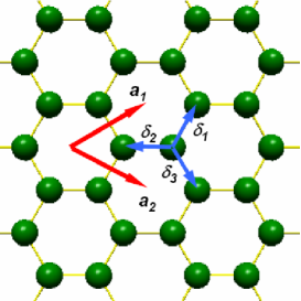
Figure 1: (Color online) The honeycomb lattice of graphene.

The hopping parameter $t$ of graphene is $t\sim 2.7eV$. The next-to-nearest neighbor hopping $t^{\prime}$ is estimated to be much smaller Ohta et al. (2007) and it will be ignored. Due to the special topology of the honeycomb lattice with two atoms per unit cell the Hamiltonian is a $2\times 2$ matrix. We will work out in some detail the different terms. The operators $\hat{a},\hat{b}$ associated to the two triangular sublattices A, B are

$$a^{+}_{iA\sigma}=\frac{1}{\sqrt{N_{A}}}\sum_{k}e^{i{\bf k.R_{iA}}}a^{+}_{{\bf k}\sigma}\;\;\;,\;\;\;b^{+}_{iB\sigma}=\frac{1}{\sqrt{N_{B}}}\sum_{k}e^{i{\bf k.R_{iB}}}b^{+}_{{\bf k}\sigma}\;\;\;,\;\;\;\vec{R}_{iA}=\vec{R}_{iB}+\vec{\delta},$$ (2)

where $N_{A}=N_{B}=N$ is the number of lattice cells and $\delta_{i}$ are the three vectors connecting a point of sublattice A with its three neighbors in sublattice B (see Fig. 1).

In term of these operators the free Hamiltonian reads

$$H_{0}=t\sum_{k\sigma}[\phi({\bf k})a^{+}_{k\sigma}b_{k\sigma}+\phi^{*}({\bf k})b^{+}_{k\sigma}a_{k\sigma}]+\mu\sum_{k\sigma}(a^{+}_{k\sigma}a_{k\sigma}+b^{+}_{k\sigma}b_{k\sigma}),$$ (3)

where we have included a chemical potential $\mu$.

In matrix form the non–interacting Hamiltonian is

$$H_{0}=\left(\begin{array}[]{cc}\mu&t\phi({\bf k})\\ t\phi^{*}({\bf k})&\mu\\ \end{array}\right),$$ (6)

where

$$\phi(\vec{k})=\sum_{i}e^{-i\vec{k}.\vec{\delta}_{i}},$$ (7)

The Hamiltonian (6) gives rise to the dispersion relation

$$\varepsilon^{0}({\bf k})=\mu\pm t\sqrt{|\phi(\vec{k})|^{2}}=\mu\pm t\sqrt{1+4\cos^{2}\frac{\sqrt{3}}{2}ak_{x}+4\cos\frac{\sqrt{3}}{2}ak_{x}\cos\frac{3}{2}ak_{y}}\;,$$ (8)

whose lower band is shown in the left hand side of Fig. 2.

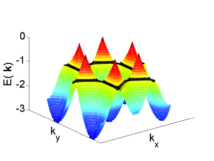
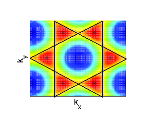
Figure 2: (Color online) Left: Lower band of the dispersion relation of graphene. The black line marks the Fermi surface for the Van Hove filling. Right: Evolution of the Fermi surface of graphene with doping. At half filling the Fermi surface consists on the six vertices of the hexagonal Brillouin zone (black points). Only two are independent, the rest being equivalent by lattice vectors. Emptying the half filled band the Fermi surface develops circular hole pockets that undergo the trigonal distortion (in red) and become the yellow triangles at the Van Hove fillig $\mu=t$.

III Coulomb interaction V and Pomeranchuk instability

We will begin by studying the influence of the interaction $V$ omitting the spin of the electrons. The on-site U will be added to study the competition of the Pomeranchuk instability with ferromagnetism. The interaction V takes place between nearest neighbors belonging to opposite sublattices. It reads:

$$H_{V}=V\sum_{{\bf kk^{\prime}q}}[a^{+}_{\bf k}a_{{\bf k+q}}b^{+}_{{\bf k^{\prime}}}b_{{\bf k^{\prime}-q}}\phi^{*}({\bf q})+b^{+}_{{\bf k}}b_{{\bf k+q}}a^{+}_{{\bf k^{\prime}}}a_{{\bf k^{\prime}-q}}\phi({\bf q})].$$ (9)

The mean field Hamiltonian becomes

$$H_{MF}=\sum_{\bf k}[\tilde{\phi}({\bf k})a^{+}_{{\bf k}}b_{{\bf k}}+\tilde{\phi}^{*}({\bf k})b^{+}_{{\bf k}}a_{\bf k}]+\mu\sum_{\bf k}(a^{+}_{\bf k}a_{\bf k}+b^{+}_{\bf k}b_{\bf k}),$$ (10)

where

$$\tilde{\phi}({\bf k})=t\phi({\bf k})-\sum_{{\bf q}}V^{*}({\bf q})<b^{+}_{{\bf k+q}}a_{{\bf k+q}}>\;\;\;,\;\;\;V({\bf q})=\frac{V}{N}\sum_{{\bf q}}\phi^{*}({\bf q}),$$ (11)

and $N$ is the number of lattice cells. In matrix form and including the chemical potential the mean field Hamiltonian reads:

$$H_{MF}=\left(\begin{array}[]{cc}\mu&t\phi({\bf k})-\sum_{\bf q}V^{*}({\bf q})<b^{+}_{k+q}a_{k+q}>\\ t\phi^{*}({\bf k})-\sum_{\bf q}V({\bf q})<a^{+}_{k+q}b_{k+q}>&\mu\\ \end{array}\right).$$ (14)

The mean field Hamiltonian (14) gives rise to the dispersion relation

$$E({\bf k})=\mu\pm[t^{2}|\phi({\bf k})|^{2}+F(V,{\bf k})]^{1/2},$$ (15)

where $F(V,{\bf k})$ is

$$F(V,{\bf k}) =-tV\sum_{{\bf q}}\phi^{*}({\bf k})\phi({\bf q})<a^{+}_{k+q}b_{k+q}>-tV\sum_{{\bf q}}\phi({\bf k})\phi^{*}({\bf q})<b^{+}_{k+q}a_{k+q}>$$

$$+V^{2}\sum_{{\bf qq^{\prime}}}\phi^{*}({\bf q})\phi({\bf q^{\prime}})<a^{+}_{k+q}b_{k+q}><b^{+}_{k+q^{\prime}}a_{k+q^{\prime}}>.$$

We look for a self–consistent solution of eq. (15) imposing the Luttinger theorem i. e. that the area enclosed by the interacting Fermi line is the same as the one chosen as the initial condition. We begin with an initial (free) Fermi surface, as an input, add the interaction and let it evolve until a self–consistent solution is found with a given ”final” interacting Fermi surface. The important constraint is that the total number of particles should remain fixed. This procedure has been used in the same context in Valenzuela and Vozmediano (2001); Roldán et al. (2008).

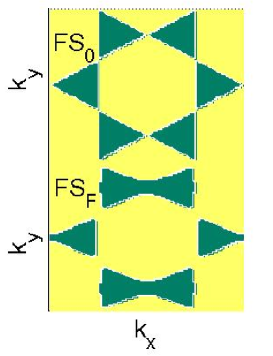
Figure 3: Pomeranchuk instability suffered by an initial Fermi surface at the Van Hove singularity (upper part) when an exchange interaction V=1t is added (lower part).

The Fermi surface of graphene around the Van Hove singularity is shown in Fig. 2. To better visualize the Pomeranchuk instability we keep the image of the neighboring Brillouin zones. Fig. 3 shows the initial Fermi surface sitting at the VHS (upper part) and the spontaneous deformation obtained self–consistently from eq. (15) for a value of the exchange interaction $V=t$.

IV Ferromagnetism and competition of ferromagnetism and Pomeranchuk instabilities

In order to study a possible ferromagnetic instability we will add to the free Hamiltonian an on–site Hubbard term

$$H_{U}=U\sum_{i}[a^{+}_{i\uparrow}a_{i\uparrow}a^{+}_{i\downarrow}a_{i\downarrow}+b^{+}_{i\uparrow}b_{i\uparrow}b^{+}_{i\downarrow}b_{i\downarrow}],$$ (17)

A mean field ferromagnetic state will be characterized by

$$a^{+}_{i\sigma}a_{i\sigma}=<a^{+}_{i\sigma}a_{i\sigma}>+\delta(a^{+}_{i\sigma}a_{i\sigma})$$ (18)

with

$$<a^{+}_{i\sigma}a_{i\sigma}>=\frac{n}{2}+\sigma\frac{m}{2}\;\;\;,\;\;\;<b^{+}_{i\sigma}b_{i\sigma}>=\frac{n}{2}+\sigma\frac{m}{2}\;\;\;,\;\;\;\sigma=\pm,$$ (19)

what produces the mean field Hamiltonian

$$H^{U}_{MF}=U\sum_{i\sigma}(\frac{n}{2}+\sigma\frac{m}{2})(a^{+}_{i\sigma}a_{i\sigma}+b^{+}_{i\sigma}b_{i\sigma})-\frac{1}{2}U(n^{2}-m^{2})N.$$ (20)

Adding the kinetic term we get the Hamiltonian

$$H_{0}+H^{U}_{MF}=\left(\begin{array}[]{cc}\mu+\frac{U}{2}(n+\sigma m)&t\phi({\bf k})\\ t\phi^{*}({\bf k})&\mu+\frac{U}{2}(n+\sigma m)\\ \end{array}\right)$$ (23)

whose dispersion relation

$$E_{k\sigma}=\mu_{\sigma}\pm t|\phi({\bf k})|\;\;\;,\;\;\;\mu_{\sigma}=\mu+\frac{U}{2}(n+\sigma m),$$ (24)

is solved self–consistently to get the ferromagnetic ground state.

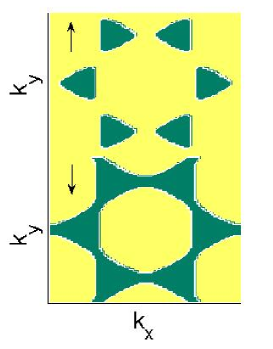
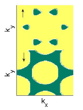
Figure 4: (Color online) Left: Initial polarization of the Fermi surface with the spin up electrons (upper part) less populated than the spin down (lower part): $n_{\downarrow}-n_{\uparrow}=0.14$, $\mu_{\uparrow}=-0.9t$, $\mu_{\downarrow}=-1.1t$. Center: Final state obtained for the values of the parameters U=1t and V=2t. A Pomeranchuk instability is clearly visible in both spin bands. Right: Final state with enhanced ferromagnetic polarization obtained for the values of the parameters U=2t and V=1t.

The competition of the Pomeranchuk instability found in the previous section with a possible ferromagnetic instability is studied with the same procedure using the full mean field Hamiltonian $H_{0}+H^{V}_{MF}+H^{U}_{MF}$ and solving self-consistently the equations

$$E_{\uparrow}({\bf k})=\mu+Un_{\downarrow}-\sqrt{t^{2}|\phi({\bf k})|^{2}+F(V,{\bf k})_{\uparrow}},$$ (25)

$$E_{\downarrow}({\bf k})=\mu+Un_{\uparrow}-\sqrt{t^{2}|\phi({\bf k})|^{2}+F(V,{\bf k})_{\downarrow}},$$ (26)

where $F(V,{\bf k})_{\sigma}$ is given in eq. (12) and $n_{\sigma}=1/2(n+\sigma m)$.

V Summary of the results

The competition of the Pomeranchuk instability with ferromagnetism is exemplified in Fig. 4. The figure in the left side represents the initial free Fermi surface where the spin up (upper side) and down (lower side) electrons have different populations around the Van Hove filling. In particular in the example given, the chemical potential of the spin up (down) electrons is set slightly below (above) the VHS: $n_{\downarrow}-n_{\uparrow}=0.14$, $\mu_{\uparrow}=-0.9t$, $\mu_{\downarrow}=-1.1t$. The image in the center represents the renormalized Fermi surface for the two spin polarizations when the exchange interaction V is bigger than U: $V=2U=2t$. We can see that the ferromagnetism has disappeared: the final Fermi surface is the same for the two spin polarization and presents a Pomeranchuk deformation. The opposite case is shown in the figure at the right: with the same initial configuration the final state for the values of the interactions $U=2V=2t$ has an enhanced ferromagnetism with no signal of deformation.

The phase diagram of the dominant instability as a function of the interaction strength U and V (measured in units of the hopping parameter t) is shown in Fig. 5. In all cases the initial Fermi surface consists of a slightly polarized state around the Van Hove singularity as the one shown in the left hand side of Fig. 4. The symbols in Fig. 5 denote calculated points with the following meaning: the circles appearing for low values of U denote an unpolarized final state with Pomeranchuk deformation as the one shown in the center of Fig. 4. Crosses appearing for large values of U represent a final state where the polarization is bigger than the initial one and the Fermi surface has the original symmetry as the one in the right hand side of Fig. 4. The points denoted by $\bigotimes$ correspond to values where both instabilities coexist and the final Fermi surface is deformed and spin polarized. Finally the crosses at low values of U with V=0 represent final states which are still polarized but where the spin polarization is smaller than the initial one. This region is denoted by $FM\downarrow$ in the figure phase diagram. PI (FM) denotes the region where the Pomeranchuk (ferromagnetic) instability dominated respectively.

The ferromagnetic evolution of the system for V=0 is as follows: Below a critical value of $1.5<U_{c}<2$ a free slightly polarized system at fillings near (but not at) the VHS evolves towards an unpolarized one in agreement with Peres et al. (2004); Araujo and Peres (2006). The Coulomb exchange V induces a deformation of the Fermi surface already at very small values $V_{c}\sim 0.4t$ when the free initial state is near the Van Hove singularity. Increasing U enhances the magnetic polarization of the interacting system until the critical value $U\sim 1.75t$ is reached where the final state corresponds to a ferromagnetic system with un-deformed Fermi surface. Unlike what happens in the square lattice, the critical value of U above which ferromagnetism prevails does not depend on V (vertical line in Fig. 5). In the blank region in the upper part of the figure corresponding to high values of V around the critical U we have not been able to reach a self–consistent solution.

We note that at V=0, the critical U for ferromagnetism is zero at the Van Hove filling and changes very rapidly around it in a rigid band model Peres et al. (2004); Araujo and Peres (2006). This behavior is due to the divergent density of states at the VHS that would be smeared by temperature effects or disorder in real samples. Based on the previous studies if the square lattice we are confident that the results obtained in the present work are robust and the phase diagram shown in fig. 5 will remain qualitatively when more detailed calculations are done.

The realization of one or another phase in real graphene samples depends on the values that the effective Coulomb interaction parametrized by $U,V$ has at the VHS filling. Besides the ARPES experiments Chesney et al. (2007) which do not comment on the strength of the interaction, we are not aware of other experiments at these doping levels. Conservative estimates can be obtained from the graphite intercalated compounds Tchougreeff and Hoffmann (1992) on the basis of the similarities found in Chesney et al. (2007) between the Fermi surfaces of the two. Values of $U\sim 2.5t$, $V\sim t$ can be very reasonable and lie in the range discussed in the present work.

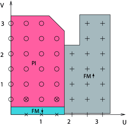
Figure 5: Phase diagram showing the competition of Pomeranchuk and ferromagnetic instabilities as a function of the interactions U and V measured in units of the hopping parameter t.

VI Discussion and open problems

In this work we have examined some physical issues to be expected in graphene at high doping. We have seen that at the Van Hove filling in the presence of an exchange Coulomb interaction the Fermi surface is softer and becomes very easily deformed as compared with a similar analysis of the square lattice.

A natural extension of the work presented in this article is to study the competition of the instabilities studied in this work with superconductivity along the lines of ref. Yamase and Metzner (2007). A complete renormalization group analysis of the competing low energy instabilities of the Van Hove filling as a function of the doping and the couplings U and V is also to be done. Due to the special geometry of the Fermi surface in the honeycomb lattice the symmetry breaking phases can present a richer variety than those of the square lattice. A fairly complete analysis of the short range interactions around the Dirac point was done in the early paper González et al. (2001). Due to the existence of two Fermi points the classification of the possible low–energy couplings is similar to the g–ology of the one dimensional models. The RG classification of the low–energy couplings in the Van Hove filling is richer since there are three independent VH points to consider and work in this direction is in progress. An analysis of the physics of the Fermi surface around the trigonal warping can lead also to very interesting results in the light of the evolution of the Fermi surface anisotropies done in González et al. (1997); Roldán et al. (2006).

On the view of the analysis of this problem done in the square lattice we can expect that RG calculation will enrich the phase diagram but the two phases discussed here will stay. Ferromagnetism is a likely possibility due to the Stoner criterium although it will compete with antiferromagnetism at high values of U. A very important parameter to this problem is the next to nearest neighbor hopping $t^{\prime}$ that suppresses the nesting of the bare Fermi surface and affects the shape of the phase transition lines Peres et al. (2004); Araujo and Peres (2006). These references focuss on the magnetism of the Hubbard model (U) on the honeycomb lattice at finite dopings and found that non–homogeneous (spiral) phases are the most stable configurations around the Van Hove filling. It would be interesting to analyze the competition and stability of these non–homogeneous ferromagnetic configurations in the presence of a V interaction.

Of particular interest is the possibility of coexistence or competition of the Pomeranchuk instability with possible superconducting instabilities González (2008). A very interesting suggestion has been made in studies of the square lattice that superconductivity changes the nature of the Pomeranchuk transition going from first to second order Yamase and Metzner (2007). This feature will probably be maintained in the honeycomb lattice and we are actually exploring this problem.

As it is known, the Kohn–Luttinger instability in its original context Kohn and Luttinger (1965) suggests that no Fermi liquid will be stable at sufficiently low temperatures. In the case of a 3D electron system with isotropic Fermi surface there is an enhanced scattering at momentum transfer $2k_{F}$ which translates into a modulation of the effective interaction potential with oscillating behavior similar to the Friedel oscillations. This makes possible the existence of attractive channels, labelled by the angular momentum quantum number. The issue of the stability of Fermi liquids was studied rigorously in two dimensions in a set of papers Feldman et al. (2004a, b, c) with the conclusion that a Fermi liquid could exist in two space dimensions at zero temperature provided that the Fermi surface of the system obeys some ”asymmetry” conditions. In particular the non–interacting Fermi surface had to lack inversion symmetry

$$\epsilon(-{\bf k})\neq\epsilon({\bf k})$$

at all points k and be otherwise quite regular (the Van Hove singularities can not be present). The dispersion relation of graphene obeys such a condition for fillings where the trigonal warping is already noticeable and below the Van Hove filling provided that disorder and interactions do not mix the Van Hove points. This is a very common assumption in the graphene physics around the Dirac points where the inversion symmetry in k–space acts as a time reversal symmetry Mañes et al. (2007). We find interesting to note that the –quite restrictive–conditions of refs. Feldman et al. (2004a, b, c) can be fulfilled in a real –and very popular–system.

VII Acknowledgments.

We thank A. Cortijo, M. P. López-Sancho and R. Roldán for very interesting discussions. This research was supported by the Spanish MECD grant FIS2005-05478-C02-01 and by the Ferrocarbon project from the European Union under Contract 12881 (NEST).

References

- Novoselov et al. (2005) K. S. Novoselov, A. K. Geim, S. V. Morozov, D. Jiang, M. I. Katsnelson, I. V. Grigorieva, S. V. Dubonos, and A. A. Firsov, Nature 438, 197 (2005).
- Zhang et al. (2005) Y. Zhang, Y.-W. Tan, H. L. Stormer, and P. Kim, Nature 438, 201 (2005).
- Semenoff (1984) G. V. Semenoff, Phys. Rev. Lett. 53, 2449 (1984).
- Haldane (1988) F. D. M. Haldane, Phys. Rev. Lett. 61, 2015 (1988).
- González et al. (1996) J. González, F. Guinea, and M. A. H. Vozmediano, Phys. Rev. Lett. 77, 3589 (1996).
- Khveshchenko (2001) D. V. Khveshchenko, Phys. Rev. Lett. 87, 246802 (2001).
- Kopelevich et al. (2003) Y. Kopelevich et al., Phys. Rev. Lett. 90, 156402 (2003).
- Novoselov et al. (2004) K. S. Novoselov et al., Science 306, 666 (2004).
- Esquinazi et al. (2003) P. Esquinazi et al., Phys. Rev. Lett. 91, 227201 (2003).
- Chesney et al. (2007) J. L. M. Chesney, A. Bostwick, T. Ohta, K. V. Emtsev, T. Seyller, K. Horn, and E. Rotenberg (2007), eprint arXiv:0705.3264.
- Bostwick et al. (2007) A. Bostwick, T. Ohta, T. Seyller, K. Horn, and E. Rotenberg, Nat. Phys. 3, 36 (2007).
- Ezawa (2007) M. Ezawa, Physica Status Solidi (c) 4, 489 (2007).
- Nemec et al. (2008) N. Nemec, K. Richter, and G. Cuniberti, New J. Phys. 10, 065014 (2008).
- Kim et al. (1999) P. Kim, T. W. Odom, J.-L. Huang, and C. M. Lieber, Phys. Rev. Lett. 82, 1225 (1999).
- González et al. (1994) J. González, F. Guinea, and M. A. H. Vozmediano, Nucl. Phys. B 424 [FS], 595 (1994).
- González et al. (1999) J. González, F. Guinea, and M. A. H. Vozmediano, Phys. Rev. B 59, R2474 (1999).
- Peres et al. (2005) N. M. R. Peres, F. Guinea, and A. H. Castro Neto, Phys. Rev. B 72, 174406 (2005).
- González et al. (2001) J. González, F. Guinea, and M. A. H. Vozmediano, Phys. Rev. B 63, 134421 (2001).
- Uchoa and Castro Neto (2007) B. Uchoa and A. H. Castro Neto, Phys. Rev. Lett. 98, 146801 (2007).
- Honerkamp (2008) C. Honerkamp, Phys. Rev. Lett. 100, 146404 (2008).
- Markiewicz (1997) R. S. Markiewicz, Journal of Physics and Chemistry of Solids 58, 1179 (1997).
- González (2008) J. González (2008), eprint arXiv:0807.3914.
- González et al. (2000) J. González, F. Guinea, and M. A. H. Vozmediano, Phys. Rev. Lett. 84, 4930 (2000).
- Pomeranchuk (1958) I. Pomeranchuk, Zh. Eksp. Teor. Fiz. 35, 524 (1958), [Sov. Phys. JETP 8, 361 (1959)].
- Halboth and Metzner (2000) C. J. Halboth and W. Metzner, Phys. Rev. Lett. 85, 5162 (2000).
- Valenzuela and Vozmediano (2001) B. Valenzuela and M. A. H. Vozmediano, Phys. Rev. B 63, 153103 (2001).
- González (2001) J. González, Phys. Rev. B 63, 045114 (2001).
- recent approach to the subject et al. (2008) A. recent approach to the subject, a complete list of references can be found in C.A. Lamas, D. Cabra, and N. Grandi (2008), eprint arXiv:0804.4422.
- Yamase and Kohno (2000a) H. Yamase and H. Kohno, Journal of the Physical Society of Japan 69, 332 (2000a).
- Yamase and Kohno (2000b) H. Yamase and H. Kohno, Journal of the Physical Society of Japan 69, 2151 (2000b).
- Yamase (2008) H. Yamase (2008), eprint arXiv:0806.2226.
- Varma (2003) C. M. Varma, Phil. Mag. 85, 1657 (2003).
- Nilsson and Castro Neto (2005) J. Nilsson and A. H. Castro Neto, Phys. Rev. B 72, 195104 (2005).
- Kohn and Luttinger (1965) W. Kohn and J. M. Luttinger, Phys. Rev. Lett. 15, 524 (1965).
- Feldman et al. (2004a) J. Feldman, H. Knorrer, and E. Trubowitz, Comm. Math. Phys. 247, 1 (2004a).
- Feldman et al. (2004b) J. Feldman, H. Knorrer, and E. Trubowitz, Comm. Math. Phys. 247, 49 (2004b).
- Feldman et al. (2004c) J. Feldman, H. Knorrer, and E. Trubowitz, Comm. Math. Phys. 247, 113 (2004c).
- Luttinger (1960) J. M. Luttinger, Phys. Rev. 119, 1153 (1960).
- Roldán et al. (2008) R. Roldán, M. López-Sancho, and F. Guinea, Phys. Rev. B 77, 115410 (2008).
- Ohta et al. (2007) T. Ohta, A. Bostwick, J. L. McChesney, T. Seyller, K. Horn, and E. Rotenberg, Phys. Rev. Lett 98, 206802 (2007).
- Peres et al. (2004) N. M. R. Peres, M. A. N. Araujo, and D. Bozi, Phys. Rev. B 70, 195122 (2004).
- Araujo and Peres (2006) M. A. N. Araujo and N. M. R. Peres, Journal of Physics: Condensed Matter 18, 1769 (2006).
- Tchougreeff and Hoffmann (1992) A. L. Tchougreeff and R. Hoffmann, J. Phys. and Chem. 96, 8993 (1992).
- Yamase and Metzner (2007) H. Yamase and W. Metzner, Phys. Rev. B 75, 155117 (2007).
- González et al. (1997) J. González, F. Guinea, and M. Vozmediano, Phys. Rev. Lett. 79, 3514 (1997).
- Roldán et al. (2006) R. Roldán, M. López-Sancho, F. Guinea, and S.-W. Tsai, Phys. Rev. B 74, 235109 (2006).
- Mañes et al. (2007) J. L. Mañes, F. Guinea, and M. A. H. Vozmediano, Phys. Rev. B 75, 155424 (2007).