Scattering Theory of Gilbert Damping

Abstract

The magnetization dynamics of a single domain ferromagnet in contact with a thermal bath is studied by scattering theory. We recover the Landau-Liftshitz-Gilbert equation and express the effective fields and Gilbert damping tensor in terms of the scattering matrix. Dissipation of magnetic energy equals energy current pumped out of the system by the time-dependent magnetization, with separable spin-relaxation induced bulk and spin-pumping generated interface contributions. In linear response, our scattering theory for the Gilbert damping tensor is equivalent with the Kubo formalism.

Magnetization relaxation is a collective many-body phenomenon that remains intriguing despite decades of theoretical and experimental investigations. It is important in topics of current interest since it determines the magnetization dynamics and noise in magnetic memory devices and state-of-the-art magnetoelectronic experiments on current-induced magnetization dynamics Stiles:top06 . Magnetization relaxation is often described in terms of a damping torque in the phenomenological Landau-Lifshitz-Gilbert (LLG) equation

$$\frac{1}{\gamma}\frac{d\mathbf{M}}{d\tau}=-\mathbf{M}\times\mathbf{H}_{\mathrm{eff}}+\mathbf{M}\times\left[\frac{\tilde{G}(\mathbf{M})}{\gamma^{2}M_{s}^{2}}\frac{d\mathbf{M}}{d\tau}\right]\text{,}$$ (1)

where $\mathbf{M}$ is the magnetization vector, $\gamma=g\mu_{B}/\hbar$ is the gyromagnetic ratio in terms of the $g$ factor and the Bohr magneton $\mu_{B}$, and $M_{s}=|\mathbf{M}|$ is the saturation magnetization. Usually, the Gilbert damping $\tilde{G}(\mathbf{M})$ is assumed to be a scalar and isotropic parameter, but in general it is a symmetric $3\times 3$ tensor. The LLG equation has been derived microscopically Heinrich:pss67 and successfully describes the measured response of ferromagnetic bulk materials and thin films in terms of a few material-specific parameters that are accessible to ferromagnetic-resonance (FMR) experiments Bland:book05 . We focus in the following on small ferromagnets in which the spatial degrees of freedom are frozen out (macrospin model). Gilbert damping predicts a stricly linear dependence of FMR linewidts on frequency. This distinguishes it from inhomogenous broadening associated with dephasing of the global precession, which typically induces a weaker frequency dependence as well as a zero-frequency contribution.

The effective magnetic field $\mathbf{H}_{\mathrm{eff}}=-\partial F/\partial\mathbf{M}$ is the derivative of the free energy $F$ of the magnetic system in an external magnetic field $\mathbf{H}_{\mathrm{ext}}$, including the classical magnetic dipolar field $\mathbf{H}_{d}$. When the ferromagnet is part of an open system as in Fig. 1, $-\partial F/\partial\mathbf{M}$ can be expressed in terms of a scattering S-matrix, quite analogous to the interlayer exchange coupling between ferromagnetic layers Bruno:prb95 . The scattering matrix is defined in the space of the transport channels that connect a scattering region (the sample) to thermodynamic (left and right) reservoirs by electric contacts that are modeled by ideal leads. Scattering matrices also contain information to describe giant magnetoresistance, spin pumping and spin battery, and current-induced magnetization dynamics in layered normal-metal (N)$\mid$ferromagnet (F) systems Bruno:prb95 ; Waintal:prb00 ; Tserkovnyak:prl02 .

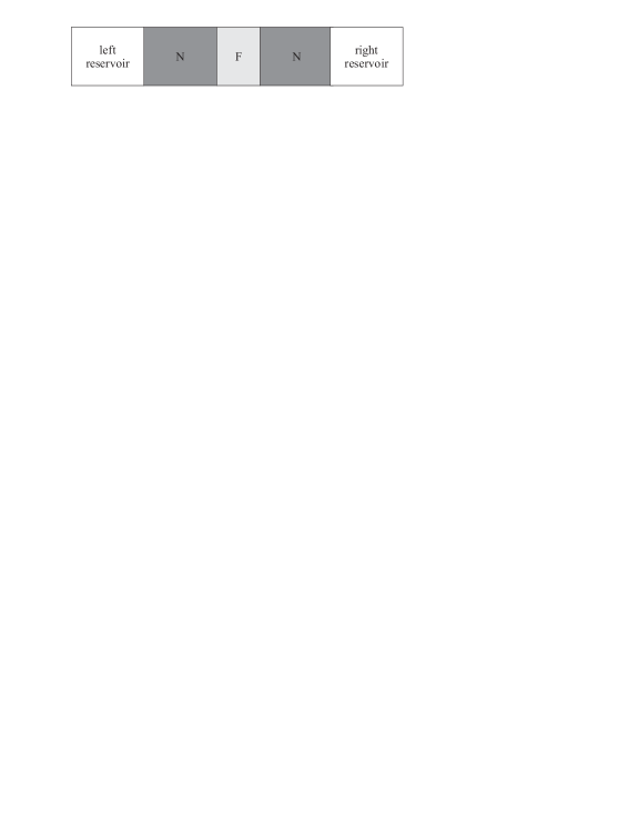
Figure 1: Schematic picture of a ferromagnet (F) in contact with a thermal bath via metallic normal metal leads (N).

In the following we demonstrate that scattering theory can be also used to compute the Gilbert damping tensor $\tilde{G}(\mathbf{M}).$ The energy loss rate of the scattering region can be described in terms of the time-dependent S-matrix. Here, we generalize the theory of adiabatic quantum pumping to describe dissipation in a metallic ferromagnet. Our idea is to evaluate the energy pumping out of the ferromagnet and to relate this to the energy loss of the LLG equation. We find that the Gilbert phenomenology is valid beyond the linear response regime of small magnetization amplitudes. The only approximation that is necessary to derive Eq. (1) including $\tilde{G}(\mathbf{M})$ is the (adiabatic) assumption that the frequency $\omega$ of the magnetization dynamics is slow compared to the relevant internal energy scales set by the exchange splitting $\Delta$. The LLG phenomenology works so well because $\hbar\omega\ll\Delta$ safely holds for most ferromagnets.

Gilbert damping in transition-metal ferromagnets is generally believed to stem from spin-orbit interaction in combination with impurity scattering that transfers magnetic energy to itinerant quasiparticles Bland:book05 . The subsequent drainage of the energy out of the electronic system, e.g. by inelastic scattering via phonons, is believed to be a fast process that does not limit the overall damping. Our key assumption is adiabaticiy, meaning that the precession frequency goes to zero before letting the sample size become large. The magnetization dynamics then heats up the entire magnetic system by a tiny amount that escapes via the contacts. The leakage heat current then equals the total dissipation rate. For sufficiently large samples, bulk heat production is insensitive to the contact details and can be identified as an additive contribution to the total heat current that escapes via the contacts. The chemical potential is set by the reservoirs, which means that (in the absence of an intentional bias) the sample is then always very close to equilibrium. The S-matrix expanded to linear order in the magnetization dynamics and the Kubo linear response formalisms should give identical results, which we will explicitly demonstrate. The role of the infinitesimal inelastic scattering that guarantees causality in the Kubo approach is in the scattering approach taken over by the coupling to the reservoirs. Since the electron-phonon relaxation is not expected to directly impede the overall rate of magnetic energy dissipation, we do not need to explicitly include it in our treatment. The energy flow supported by the leads, thus, appears in our model to be carried entirely by electrons irrespective of whether the energy is actually carried by phonons, in case the electrons relax by inelastic scattering before reaching the leads. So we are able to compute the magnetization damping, but not, e.g., how the sample heats up by it .

According to Eq. (1), the time derivative of the energy reads

$$\dot{E}=\mathbf{H}_{\mathrm{eff}}\mathbf{\cdot}d\mathbf{M/}d\tau=(1/\gamma^{2})\mathbf{\dot{m}}\left[\tilde{G}(\mathbf{m})\mathbf{\dot{m}}\right]\mathbf{,}$$ (2)

in terms of the magnetization direction unit vector $\mathbf{m}=\mathbf{M}/M_{s}$ and $\mathbf{\dot{m}}=d\mathbf{m}/d\tau$. We now develop the scattering theory for a ferromagnet connected to two reservoirs by normal metal leads as shown in Fig. 1. The total energy pumping into both leads $I_{E}^{\mathrm{(pump)}}$ at low temperatures reads Avron:prl01 ; Moskalets:prb02

$$I_{E}^{\mathrm{(pump)}}=(\hbar/4\pi)\mathrm{Tr}\dot{S}\dot{S}^{{\dagger}},$$ (3)

where $\dot{S}=dS/d\tau$ and $S$ is the S-matrix at the Fermi energy:

$$S(\mathbf{m})=\left(\begin{array}[c]{cc}r&t^{\prime}\\ t&r^{\prime}\end{array}\right)\,.$$ (4)

$r$ and $t$ ($r^{\prime}$ and $t^{\prime}$) are the reflection and transmission matrices spanned by the transport channels and spin states for an incoming wave from the left (right). The generalization to finite temperatures is possible but requires knowledge of the energy dependence of the S-matrix around the Fermi energy Moskalets:prb02 . The S-matrix changes parametrically with the time-dependent variation of the magnetization $S(\tau)=S(\mathbf{m}(\tau))$. We obtain the Gilbert damping tensor in terms of the S-matrix by equating the energy pumping by the magnetic system (3) with the energy loss expression (2), $\dot{E}=I_{E}^{\text{(pump)}}$. Consequently

$$G_{ij}(\mathbf{m})=\frac{\gamma^{2}\hbar}{4\pi}\operatorname{Re}\left\{\mathrm{Tr}\left[\frac{\partial S}{\partial m_{i}}\frac{\partial S^{{\dagger}}}{\partial m_{j}}\right]\right\}\,,$$ (5)

which is our main result.

The remainder of our paper serves three purposes. We show that (i) the S-matrix formalism expanded to linear response is equivalent to Kubo linear response formalism, demonstrate that (ii) energy pumping reduces to interface spin pumping in the absence of spin relaxation in the scattering region, and (iii) use a simple 2-band toy model with spin-flip scattering to explicitly show that we can identify both the disorder and interface (spin-pumping) magnetization damping as additive contributions to the Gilbert damping.

Analogous to the Fisher-Lee relation between Kubo conductivity and the Landauer formula Fisher:prb81 we will now prove that the Gilbert damping in terms of S-matrix (5) is consistent with the conventional derivation of the magnetization damping by the linear response formalism. To this end we chose a generic mean-field Hamiltonian that depends on the magnetization direction $\mathbf{m}$: $\hat{H}=\hat{H}(\mathbf{m})$ describes the system in Fig. 1. $\hat{H}$ can describe realistic band structures as computed by density-functional theory including exchange-correlation effects and spin-orbit coupling as well normal and spin-orbit induced scattering off impurities. The energy dissipation is $\dot{E}=\langle d\hat{H}/d\tau\rangle$, where $\langle\dots\rangle$ denotes the expectation value for the non-equilibrium state. In linear response, we expand the magnetization direction $\mathbf{m}(t)$ around the equilibrium magnetization direction $\mathbf{m}_{0}$,

$$\mathbf{m}(\tau)\mathbf{=m}_{0}+\mathbf{u}(\tau).$$ (6)

The Hamiltonian can be linearized as $\hat{H}=\hat{H}_{\mathrm{st}}+u_{i}(\tau)\partial_{i}\hat{H}$, where $\hat{H}_{\mathrm{st}}\equiv\hat{H}(\mathbf{m}_{0})$ is the static Hamiltonian and $\partial_{i}\hat{H}\equiv\partial_{u_{i}}\hat{H}(\mathbf{m}_{0})$, where summation over repeated indices $i=x,y,z$ is implied. To lowest order $\dot{E}=\dot{u}_{i}(\tau)\langle\partial_{i}\hat{H}\rangle$, where

$$\langle\partial_{i}\hat{H}\rangle=\langle\partial_{i}\hat{H}\rangle_{0}+\int_{-\infty}^{\infty}d\tau^{\prime}\chi_{ij}(\tau-\tau^{\prime})u_{j}(\tau^{\prime})\,.$$ (7)

$\langle\dots\rangle_{0}$ denotes equilibrium expectation value and the retarded correlation function is

$$\chi_{ij}(\tau-\tau^{\prime})=-\frac{i}{\hbar}\theta(\tau-\tau^{\prime})\left\langle[\partial_{i}\hat{H}(\tau),\partial_{j}\hat{H}(\tau^{\prime})]\right\rangle_{0}\,$$ (8)

in the interaction picture for the time evolution. In order to arrive at the adiabatic (Gilbert) damping the magnetization dynamics has to be sufficiently slow such that $u_{j}(\tau)\approx u_{j}(t)+\left(\tau-t\right)\dot{u}_{j}(t)$. Since $\mathbf{m}^{2}=1$ and hence $\mathbf{\dot{m}\cdot m}=0$ Simanek:prb03

$$\dot{E}=i\partial_{\omega}\chi_{ij}(\omega\rightarrow 0)\dot{u}_{i}\dot{u}_{j},$$ (9)

where $\chi_{ij}(\omega)=\int_{-\infty}^{\infty}d\tau\chi_{ij}(\tau)\exp(i\omega\tau)$.  Next, we use the scattering states as the basis for expressing the correlation function (8). The Hamiltonian consists of a free-electron part and a scattering potential: $\hat{H}=\hat{H}_{0}+\hat{V}(\mathbf{m})$. We denote the unperturbed eigenstates of the free-electron Hamiltonian $\hat{H}_{0}=-\hbar^{2}\nabla^{2}/2m$ at energy $\epsilon$ by $|\varphi_{s,q}(\epsilon)\rangle$, where $s=l,r$ denotes propagation direction and $q$ transverse quantum number. The potential $\hat{V}(\mathbf{m})$ scatters the particles between these free-electron states. The outgoing (+) and incoming wave (-) eigenstates $|\psi_{s,q}^{(\pm)}(\epsilon)\rangle$ of the static Hamiltonian $\hat{H}_{\mathrm{st}}$ fulfill the completeness conditions $\langle\psi_{s,q}^{(\pm)}(\epsilon)|\psi_{s^{\prime},q^{\prime}}^{(\pm)}(\epsilon^{\prime})\rangle=\delta_{s,s^{\prime}}\delta_{q,q^{\prime}}\delta(\epsilon-\epsilon^{\prime})$ MelloKumar:book04 . These wave functions can be expressed as $|\psi_{s}^{(\pm)}(\epsilon)\rangle=[1+\hat{G}_{\mathrm{st}}^{(\pm)}\hat{V}_{\mathrm{st}}]|\varphi_{s}(\epsilon)\rangle$, where the static retarded (+) and advanced (-) Green functions are $\hat{G}_{\mathrm{st}}^{(\pm)}(\epsilon)=(\epsilon\pm i\eta-\hat{H}_{\mathrm{st}})^{-1}$ and $\eta$ is a positive infinitesimal. By expanding $\chi_{ij}(\omega)$ in the basis of the outgoing wave functions $|\psi_{s}^{(+)}\rangle$, the low-temperature linear response leads to the following energy dissipation (9) in the adiabatic limit

$$\dot{E}=-\pi\hbar\dot{u}_{i}\dot{u}_{j}\left\langle\psi_{s,q}^{(+)}|\partial_{i}\hat{H}|\psi_{s^{\prime},q^{\prime}}^{(+)}\right\rangle\left\langle\psi_{s^{\prime},q^{\prime}}^{(+)}|\partial_{j}\hat{H}|\psi_{s,q}^{(+)}\right\rangle\,,$$ (10)

with wave functions evaluated at the Fermi energy $\epsilon_{F}$.

In order to compare the linear response result, Eq. (10), with that of the scattering theory, Eq. (5), we introduce the T-matrix $\hat{T}$ as $\hat{S}(\epsilon;\mathbf{m})=1-2\pi i\hat{T}(\epsilon;\mathbf{m})$, where $\hat{T}=\hat{V}[1+\hat{G}^{(+)}\hat{T}]$ in terms of the full Green function $\hat{G}^{(+)}(\epsilon,\mathbf{m})=[\epsilon+i\eta-\hat{H}(\mathbf{m})]^{-1}$. Although the adiabatic energy pumping (5) is valid for any magnitude of slow magnetization dynamics, in order to make connection to the linear-response formalism we should consider small magnetization changes to the equilibrium values as described by Eq. (6). We then find

$$\partial_{\tau}\hat{T}=\left[1+\hat{V}_{\mathrm{st}}\hat{G}_{\mathrm{st}}^{(+)}\right]\dot{u}_{i}\partial_{i}\hat{H}\left[1+\hat{G}_{\mathrm{st}}^{(+)}\hat{V}_{\mathrm{st}}\right]\,.$$ (11)

into Eq. (5) and using the completeness of the scattering states, we recover Eq. (10).

Our S-matrix approach generalizes the theory of (nonlocal) spin pumping and enhanced Gilbert damping in thin ferromagnets Tserkovnyak:prl02 : by conservation of the total angular momentum the spin current pumped into the surrounding conductors implies an additional damping torque that enhances the bulk Gilbert damping. Spin pumping is an N$\mid$F interfacial effect that becomes important in thin ferromagnetic films Heinrich:prl03 . In the absence of spin relaxation in the scattering region, the S-matrix can be decomposed as $S(\mathbf{m})=S_{\uparrow}(1+\hat{\boldsymbol{\sigma}}\cdot\mathbf{m})/2+S_{\downarrow}(1-\hat{\boldsymbol{\sigma}}\cdot\mathbf{m})/2$, where $\hat{\boldsymbol{\sigma}}$ is a vector of Pauli matrices. In this case, $\mathrm{Tr}$ $\left(\partial_{\tau}S\right)\left(\partial_{\tau}S\right)^{\dagger}=A_{r}\mathbf{\dot{m}}^{2}$, where $A_{r}=\mathrm{Tr}[1-\operatorname{Re}S_{\uparrow}S_{\downarrow}^{{\dagger}}]$ and the trace is over the orbital degrees of freedom only. We recover the diagonal and isotropic Gilbert damping tensor: $G_{ij}=\delta_{ij}G$ derived earlier Tserkovnyak:prl02 , where

$$G=\gamma M_{s}\alpha=\frac{\left(g\mu_{B}\right)^{2}}{4\pi\hbar}A_{r}\,.$$ (12)

Finally, we illustrate by a model calculation that we can obtain magnetization damping by both spin-relaxation and interface spin-pumping from the S-matrix. We consider a thin film ferromagnet in the two-band Stoner model embedded in a free-electron metal

$$\hat{H}=-\frac{\hbar^{2}}{2m}\nabla^{2}+\delta(x)\hat{V}(\boldsymbol{\rho})\,,$$ (13)

where the in-plane coordinate of the ferromagnet is $\boldsymbol{\rho}$  and the normal coordinate is $x.$ The spin-dependent potential $\hat{V}(\boldsymbol{\rho})$ consists of the mean-field exchange interaction oriented along the magnetization direction $\mathbf{m}$ and magnetic disorder in the form of magnetic impurities $\mathbf{S}_{i}$

$$\hat{V}(\boldsymbol{\rho})=\nu\hat{\boldsymbol{\sigma}}\cdot\mathbf{m}+\sum_{i}\zeta_{i}\hat{\boldsymbol{\sigma}}\cdot\mathbf{S}_{i}\delta(\boldsymbol{\rho}-\boldsymbol{\rho}_{i}),$$ (14)

which are randomly oriented and distributed in the film at $x=0$. Impurities in combination with spin-orbit coupling will give similar contributions as magnetic impurities to Gilbert damping. Our derivation of the S-matrix closely follows Ref. Brataas:prb94 . The 2-component spinor wave function can be written as $\Psi(x,\boldsymbol{\rho})=\sum_{\mathbf{k}_{\|}}c_{\mathbf{k}_{\|}}(x)\Phi_{\mathbf{k}_{\|}}(\boldsymbol{\rho})$, where the transverse wave function is $\Phi_{\mathbf{k}_{\|}}(\boldsymbol{\rho})=\exp(i\mathbf{k}_{\|}\cdot\boldsymbol{\rho})/\sqrt{A}$ for the cross-sectional area $A$. The effective one-dimensional equation for the longitudinal part of the wave function is then

$$\left[\frac{d^{2}}{dx^{2}}+k_{\bot}^{2}\right]c_{\mathbf{k}_{\|}}(x)=\sum_{\mathbf{k}_{\|}^{\prime}}\tilde{\Gamma}_{\mathbf{k}_{\|},\mathbf{k}_{\|}^{\prime}}c_{\mathbf{k}_{\|}}(0)\delta(x)\,,$$ (15)

where the matrix elements are defined by $\tilde{\Gamma}_{\mathbf{k}_{\|},\mathbf{k}_{\|}^{\prime}}=(2m/\hbar^{2})\int d\boldsymbol{\rho}\,\Phi_{\mathbf{k}_{\|}}^{\ast}(\boldsymbol{\rho})\hat{V}(\boldsymbol{\rho})\Phi_{\mathbf{k}_{\|}^{\prime}}(\boldsymbol{\rho)}$ and the longitudinal wave vector $k_{\bot}$ is defined by $k_{\bot}^{2}=2m\epsilon_{F}/\hbar^{2}-\mathbf{k}_{\|}^{2}$. For an incoming electron from the left, the longitudinal wave function is

$$c_{\mathbf{k}_{\|}s}=\frac{\chi_{s}}{\sqrt{k_{\bot}}}\left\{\begin{array}[c]{cc}e^{ik_{\bot}x}\delta_{\mathbf{k}_{\|}s,\mathbf{k}_{\|}^{\prime}s^{\prime}}+e^{-ik_{\bot}x}r_{\mathbf{k}_{\|}s,\mathbf{k}_{\|}^{\prime}s^{\prime}}&,x<0\\ e^{ik_{\bot}x}t_{\mathbf{k}_{\|}s,\mathbf{k}_{\|}^{\prime}s^{\prime}}&,x>0\end{array}\right.\,,$$ (16)

where $s=\uparrow,\downarrow$ and $\chi_{\uparrow}=(1,0)^{{\dagger}}$ and $\chi_{\downarrow}=(0,1)^{{\dagger}}$. Inversion symmetry dictates that $t^{\prime}=t$ and $r=r^{\prime}$. Continuity of the wave function requires $1+r=t$. The energy pumping (3) then simplifies to $I_{E}^{\text{(pump)}}=\hbar\mathrm{Tr}\left(\dot{t}\dot{t}^{{\dagger}}\right)/\pi$. Flux continuity gives $t=(1+i\hat{\Gamma})^{-1}$, where $\hat{\Gamma}_{\mathbf{k}_{\|}s,\mathbf{k}_{\|}^{\prime}s^{\prime}}=\chi_{s}^{{\dagger}}\hat{\Gamma}_{\mathbf{k}_{\|}s,\mathbf{k}_{\|}^{\prime}s^{\prime}}\chi_{s^{\prime}}\left(4k_{\bot}k_{\bot}\right)^{-1/2}$.

In the absence of spin-flip scattering, the transmission coefficient is diagonal in the transverse momentum: $t_{\mathbf{k}_{\|}}^{(0)}=[1-i\eta_{\bot}\mathbf{\sigma}\cdot\mathbf{m}]/(1+\eta_{\bot}^{2})$, where $\eta_{\bot}=m\nu/(\hbar^{2}k_{\bot})$. The nonlocal (spin-pumping) Gilbert damping is then isotropic, $G_{ij}(\mathbf{m})=\delta_{ij}G^{\prime}$,

$$G^{\prime}=\frac{2\nu^{2}\hbar}{\pi}\sum_{\mathbf{k}_{\|}}\frac{\eta_{\bot}^{2}}{(1+\eta_{\bot}^{2})^{2}}\,.$$ (17)

It can be shown that $G^{\prime}$ is a function of the ratio between the exchange splitting versus the Fermi wave vector, $\eta_{F}=m\nu/(\hbar^{2}k_{F})$. $G^{\prime}$ vanishes in the limits $\eta_{F}\ll 1$ (nonmagnetic systems) and $\eta_{F}\gg 1$ (strong ferromagnet).

We include weak spin-flip scattering by expanding the transmission coefficient $t$ to second order in the spin-orbit interaction, $t\approx\left[1+t_{0}i\hat{\Gamma}_{\mathrm{sf}}-\left(t_{0}i\hat{\Gamma}_{\mathrm{sf}}\right)^{2}\right]t_{0}$, which inserted into Eq. (5) leads to an in general anisotropic Gilbert damping. Ensemble averaging over all random spin configurations and positions after considerable but straightforward algebra leads to the isotropic result $G_{ij}(\mathbf{m})=\delta_{ij}G$

$$G=G^{(\text{{int}})}+G^{\prime}\,$$ (18)

where $G^{\prime}$ is defined in Eq. (17). The “bulk” contribution to the damping is caused by the spin-relaxation due to the magnetic disorder

$$G^{(\text{{int}})}=N_{s}S^{2}\zeta^{2}\xi\,,$$ (19)

where $N_{s}$ is the number of magnetic impurities, $S$ is the impurity spin, $\zeta$ is the average strength of the magnetic impurity scattering, and $\xi=\xi(\eta_{F})$ is a complicated expression that vanishes when $\eta_{F}$ is either very small or very large. Eq. (18) proves that Eq. (5) incorporates the “bulk” contribution to the Gilbert damping, which grows with the number of spin-flip scatterers, in addition to interface damping. We could have derived $G^{(\text{{int}})}$ [Eq. (19)] as well by the Kubo formula for the Gilbert damping.

The Gilbert damping has been computed before based on the Kubo formalism based on first-principles electronic band structures Gilmore:prl07 . However, the ab initio appeal is somewhat reduced by additional approximations such as the relaxation time approximation and the neglect of disorder vertex corrections. An advantage of the scattering theory of Gilbert damping is its suitability for modern ab initio techniques of spin transport that do not suffer from these drawbacks Zwierzycki:pstat:08 . When extended to include spin-orbit coupling and magnetic disorder the Gilbert damping can be obtained without additional costs according to Eq. (5). Bulk and interface contributions can be readily separated by inspection of the sample thickness dependence of the Gilbert damping.

Phonons are important for the understanding of damping at elevated temperatures, which we do not explicitly discuss. They can be included by a temperature-dependent relaxation time Gilmore:prl07 or, in our case, structural disorder. A microscopic treatment of phonon excitations requires extension of the formalism to inelastic scattering, which is beyond the scope of the present paper.

In conclusion, we hope that our alternative formalism of Gilbert damping will stimulate ab initio electronic structure calculations as a function of material and disorder. By comparison with FMR studies on thin ferromagnetic films this should lead to a better understanding of dissipation in magnetic systems.

- (1) For a review, see M. D. Stiles and J. Miltat, Top. Appl. Phys. 101, 225 (2006) , and references therein.
- (2) B. Heinrich, D. Fraitová, and V. Kamberský, Phys. Status Solidi 23, 501 (1967); V. Kambersky, Can. J. Phys. 48, 2906 (1970); V. Korenman, and R. E. Prange, Phys. Rev. B 6, 2769 (1972); V. S. Lutovinov and M. Y. Reizer, Zh. Eksp. Teor. Fiz. 77, 707 (1979) [Sov. Phys. JETP 50, 355 1979]; V. L. Safonov and H. N. Bertram, Phys. Rev. B 61, R14893 (2000). J. Kunes and V. Kambersky, Phys. Rev. B 65, 212411 (2002); V. Kambersky Phys. Rev. B 76, 134416 (2007).
- (3) J. A. C. Bland and B. Heinrich, Ultrathin Magnetic Structures III Fundamentals of Nanomagnetism, Springer Verlag, (Heidelberg, 2004).
- (4) P. Bruno, Phys. Rev. B 52, 411 (1995).
- (5) Y. Tserkovnyak, A. Brataas, and G. E. W. Bauer, Phys. Rev. Lett. 88, 117601 (2002); Y. Tserkovnyak, A. Brataas, G. E. W. Bauer, and B. I. Halperin, Rev. Mod. Phys. 77, 1375 (2005).
- (6) X. Waintal, E. B. Myers, P. W. Brouwer, and D. C. Ralph, Phys. Rev. B 62, 12317 (2000); A. Brataas, Yu. V. Nazarov, and G. E. W. Bauer, Phys. Rev. Lett. 84, 2481 (2000); A. Brataas, G. E. W. Bauer, and P. J. Kelly, Phys. Rep. 427, 157 (2006).
- (7) E. Simanek and B. Heinrich, Phys. Rev. B 67, 144418 (2003).
- (8) A. Brataas and G. E. W. Bauer, Phys. Rev. B 49, 14684 (1994).
- (9) K. Gilmore, Y. U. Idzerda, and M. D. Stiles, Phys. Rev. Lett. 99, 027204 (2007).
- (10) P. A. Mello and N. Kumar, Quantum Transport in Mesoscopic Systems, Oxford University Press (New York, 2005).
- (11) J. E. Avron, A. Elgart, G. M. Graf, and L. Sadun, Phys. Rev. Lett., 87, 236601 (2001).
- (12) M. Moskalets and M. Büttiker, Phys. Rev. B 66, 035306 (2002); Phys. Rev. B 66, 205320 (2002).
- (13) A. Brataas, Y. Tserkovnyak, G. E. W. Bauer, and B. I. Halperin, Phys. Rev. B 66, 060404(R) (2002); X. Wang, G. E. W. Bauer, B. J. van Wees, A. Brataas, and Y. Tserkovnyak, Phys. Rev. Lett. 97, 216602 (2006).
- (14) B. Heinrich, Y. Tserkovnyak, G. Woltersdorf, A. Brataas, R. Urban, and G. E. W. Bauer, Phys. Rev. Lett 90, 187601 (2003);M. V. Costache, M. Sladkov, S. M. Watts, C. H. van der Wal, and B. J. van Wees, Phys. Rev. Lett. 97, 216603 (2006); G. Woltersdorf, O. Mosendz, B. Heinrich, and C. H. Back, Phys. Rev. Lett 99, 246603 (2007).
- (15) D. S. Fisher and P. A. Lee, Phys. Rev. B 23, 6851 (1981).
- (16) M. Zwierzycki et al., Phys. Stat. Sol. B 245, 623 (2008)