Depletion theory and the precipitation of protein by polymer

Abstract

The depletion theory of nanoparticles immersed in a semidilute polymer solution is reinterpreted in terms of depleted chains of polymer segments. Limitations and extensions of mean-field theory are discussed. An explicit expression for the interaction between two small spheres is derived. The depletion free energy for a particle of general shape is given in terms of the capacitance or effective Stokes radius. This affords a close to quantitative explanation for the effect of polymer on protein precipitation.

*Electronic address: odijktcf@wanadoo.nl

$R/2a$	1	1.1	1.2	1.3	1.5	2	4	6	10
$2-C_{2}/(4\pi a)$	0.614	0.585	0.558	0.532	0.486	0.395	0.222	0.1538	0.0952

Table 1: Scaled depletion energy between two nanospheres as a function of their separation

It is difficult to set up theories of the polymer distribution near surfaces because the computed polymer inhomogeneity is sensitive to the nature of the approximations introduced. Pierre-Gilles de Gennes devoted considerable time and effort to trying to understand these problems starting with his survey 1 of forty years ago, which is still illuminating to read, and culminating in papers containing now classic ideas like self-similarity 2 and the proximal exponent 3 . His concise, powerful note 4 on polymer depletion by a small sphere was strangely neglected by the colloid community for a long time until the peculiarity of depletion on nanoscales was reassessed merely a decade ago 5 ; 6 . There has been a flurry of activity in the statistical physics of nanocolloids immersed in polymer solutions in what has been termed the protein limit (see e.g. 7 ; 8 ; 9 ; 10 ; 11 and references therein). Here, I would like to emphasize simple aspects of polymer depletion by nanoparticles in the spirit of ref. 12 .

Let us recall the argumentation introduced by de Gennes 4 to compute the free energy of depletion involved in immersing a nanosphere into a semidilute polymer solution. The solvent is not just “good” but needs to be really “excellent” (see below), i.e. the excluded volume $\beta$ between the Kuhn segments equals $A^{3}$ where $A$ is the segment length. If the radius $a$ of the sphere is larger than $A$, it is plausible to assume that $a$ and the polymer correlation length $\xi$ are the only relevant length scales in the problem. The latter is given by 13

$$\xi=A^{-5/4}\,c_{0}^{-3/4}\,,$$ (1)

where the concentration $c_{0}$ is the number of polymer segments per unit volume. For a nanosphere dissolved in a semidilute solution of low concentration, one readily has $a\!\ll\!\xi$. De Gennes then argues that there is a volume of order $a^{3}$ – independent of $\xi$ – surrounding the sphere from which polymer is depleted 4 . Hence, the number of segments depleted is of the order of $a^{3}\,c_{0}$. Since the free energy of depletion $F_{1}$ must be proportional to this number, i.e. must be proportional to the concentration $c_{0}$, one concludes that 4

$$F_{1}\simeq\left(\frac{a}{\xi}\right)^{\!4/3}\,k_{\rm B}T\,.$$ (2)

Here, $k_{\rm B}$ is Boltzmann’s constant and $T$ is the temperature.

Here, I invoke a different type of scaling argument to derive Eq.(2) because this will allow a direct assessment of the other aspects of depletion in the analysis below. The number of polymer segments depleted from the vicinity of the sphere is $a^{3}\,c_{0}$ so one might be tempted to think naively that the free energy of depletion could be something like $F_{1}\!\simeq\!a^{3}\,c_{0}\,k_{\rm B}T$. But this disregards entirely the fact that the segments are all connected (and are actually all on one single polymer chain because $a\!\ll\!\xi$). A depleted test segment is connected to $h$ others where $a\!\simeq\!h^{3/5}\,A$, in view of the excluded-volume effect. Therefore, the number of degrees of freedom is reduced by a factor $h$

$$F_{1}\simeq a^{3}\,c_{0}\,h^{-1}\,k_{\rm B}T\,,$$ (3)

which agrees with Eq.(2). Note that this derivation is valid in the mean for the effective number of degrees of freedom is actually less than unity in Eq.(3).

In the following I discuss several problems concerning the depletion interaction between nanospheres and polymer and its usefulness in explaining the precipitation of proteins by polymer.

Water is often the solvent of choice in experiments concerning the thermodynamic properties of polymer-nanocolloid or polymer-protein mixtures. Although water-soluble polymers dissolve readily in aqueous solution, the solvent must often be regarded as “intermediate” ($\beta\!\ll\!A^{3}$) rather than “excellent” 5 . The polymer chain then interacts with a nanoparticle in a quasi-ideal manner 12 .

In effect, the excluded-volume parameter $z\!=\!h^{1/2}\,\beta/A^{3}$ may remain smaller that unity if the nanoparticle is not too large. In that case, a string of depleted segments behaves like a Gaussian chain: $h\!\simeq\!a^{2}/A^{2}$ if the particle is a sphere. This would imply the condition 12 $a\!<\!A^{4}/\beta$ which may be easily met in practice. Eq.(3) then leads to 14

$$F_{1}=k_{1}\,A^{2}\,a\,c_{0}\,k_{\rm B}T=k_{1}\,\left(\frac{a}{\xi_{\rm id}}\right)\,k_{\rm B}T\,,$$ (4)

where $k_{1}$ is a numerical coefficient and $\xi_{\rm id}\!=\!1/(A^{2}c_{0})$ is a quasi-ideal correlation length. The latter relates to a state in which the polymer chains are supposed hypothetically ideal. Within the same approximation, one may argue in favor of a self-consistent field picture at $a\!\ll\!\xi$ which leads to a Laplace equation 12 for $\Psi(\vec{r})$ where the inhomogeneous polymer segment density $c(\vec{r})\!=\!c_{0}\,\Psi(\vec{r})^{2}$

$$\Delta\Psi(\vec{r})=0\,.$$ (5)

The solution to Eq.(5) with $\Psi\!=\!0$ at the boundary of the sphere is

$$\Psi(r)=1-\frac{a}{r}\,.$$ (6)

This leads to a value $k_{1}\!=\!2\pi/3$ for the coefficient in Eq.(4).

Nevertheless, this SCF point of view cannot be entirely correct. At some distance $r_{\ast}$ from the sphere, excluded volume effects must come into play in Eq.(5) but then the argumentation for a mean-field approach also becomes weak. From renormalization theory 6 , we know that in the case $\beta\!=\!A^{3}$ we have asymptotically

$$\Psi(r)-1\sim\left(\frac{a}{r}\right)^{\!\rm x}\,,$$ (7)

with exponent x $\!\simeq\!4/3$. When the solvent is intermediate ($\beta\!\ll\!A^{3}$), we again adduce reasoning based on the parameter $z$ above to show that Eq.(6) is only valid for $r\!<\!r_{\ast}\!=\!A^{4}/\beta$. Beyond $r_{\ast}$, Eq.(6) must join smoothly to

$$\Psi(r)\simeq 1-\frac{a\,A^{4/3}}{\beta^{1/3}\,\,r^{4/3}}\,.$$ (8)

This reduces to Eq.(7) if $a\!>\!r_{\ast}$.

The SCF theory for the polymer distribution near a surface is incorrect for a number of reasons. First, the correlation length $\xi$ is given by a wrong power law which de Gennes 2 proposed to amend by changing the exponent in the excluded volume term in the SCF equation. Nevertheless, the equation remains purely diffusive so it cannot mimic the segment distribution about a sphere expressed by Eq.(7). A further amendment could be to introduce a fractional SCF equation. In the vicinity of the sphere, this would reduce to

$$r^{1-D}\frac{d}{dr}\left(r^{D-1}\,r^{-\Theta}\,\frac{d\Psi}{dr}\right)=0\,,$$ (9)

which is a stationary generalized diffusion equation of fractal order $D$ and with a diffusion coefficient $r^{-\Theta}$. (For a discussion of fractional diffusion equations, see ref. 15 ). Eq.(7) imposes the constraint $D-\Theta\!=\!10/3$ on the exponents $D$ and $\Theta$, which leaves one of them to be suitably chosen. However, a fractional SCF equation is still not entirely satisfactory. Density fluctuations are merely accounted for in a preaveraged sense.

It is interesting to note that there is a relation between the depleted concentration about a sphere $c(r)-c_{0}$ and the pair correlation function $g(r)$ pertaining to a single chain in the bulk 13 (see Eqs.(6) and (7))

$$c(r)-c_{0}\simeq-c_{0}\,a^{3}\,h^{-1}\,g(r)\,.$$ (10)

This is independent of the strength of the excluded-volume effect. The structure of the depletion hole is analogous to the pair correlation structure of the polymer removed provided the latter is normalized by the effective number of degrees of freedom depleted by the sphere.

It is of interest to consider the interaction between two nanospheres separated at distance $R$ in the quasi-ideal limit. One needs to solve Eq.(5) with boundary conditions $\Psi\!=\!0$ at their surfaces and $\Psi\!=\!1$ at infinity. In the electrostatic analogy, the two spheres are grounded. This is not a trivial problem 16 . Using the method of images 17 , one proceeds as follows. A positive test charge is placed at the center of the first sphere. The potential $\Psi$ on the second sphere is brought to zero by alternately adding appropriate image charges on the center line between the two spheres: these are negative within the second sphere but positive in the first. Next, a similar test charge of positive sign is placed at the center of the second sphere. The potential on the first sphere is now rendered uniform by again adding image charges on the centerline but the signs are interchanged. The potential on both spheres is identical and uniform. Thus, we derive the capacitance of the two spheres as a series expansion which may be written in a less cumbersome manner via the method of difference equations. The depletion free energy turns out to be directly related to the capacitance of a particle 12 via Green’s first identity which finally leads to

$$\frac{F_{2}}{k_{\rm B}T} = \frac{A^{2}}{6}\,c_{0}\,(C_{2}-8\pi\,a)\,,$$ (11)

$$C_{2} = 8\pi\,a\,\sinh(\tau)\,\sum\limits_{n=1}^{\infty}\frac{(-1)^{n+1}}{\sinh(n\,\tau)}\,,$$ (12)

$$\cosh(\tau) \equiv \frac{R}{2a}\,.$$

Eq.(11) disagrees with an expression quoted by Hanke et al. without proof 18 . The function $2-C_{2}/(4\pi\,a)$ is very slowly varying (see Table 1) and has a maximum equal to $2-2\ln 2$ as the spheres touch. Here, the units for capacitance have been chosen in such a way that $C_{1}\!=\!4\pi\,a$ for a single sphere. Inevitably, Eq.(11) breaks down at separations $R$ beyond $r_{\ast}$ as the excluded-volume effect starts to play a role. Nevertheless, the decay of $F_{2}$ with $R$ is not fast enough for a finite computation of the second virial coefficient. A cut-off at $R\!\simeq\!\xi$ must be introduced as has been discussed by Eisenriegler 19 in the excellent-solvent case ($\beta\!=\!A^{3}$). The opposite limit of large spheres near ideal polymers has been addressed by Tuinier et al. 20 .

How well does an expression like Eq.(4) work? An important phenomenon bioengineering is the precipitation of proteins by inert polymer. This has been studied for a long time 21 ; 22 ; 23 ; 24 ; 25 but the most thorough quantitative study is that of Atha and Ingham 26 . They determined the solubility $S$ of a host of proteins as a function of the polyethylene glycol (PEG) added to the suspension. The concentrations of PEG were well into the semidilute regime. The logarithm of the solubility turns out to be a purely linear function of the PEG concentration and the resulting slopes are a monotone function of the protein radius, the latter being an equivalent quantity derived from the diffusion coefficient via the Stokes-Einstein relation (see Fig. 1).

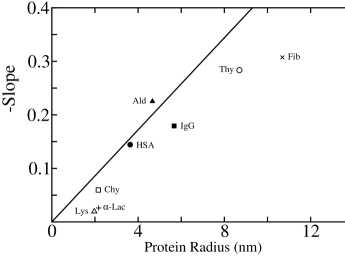
Figure 1: The slope of the linear plot of ${}^{10\!}\log S$ versus $w$ as a function of the effective Stokes radius of various proteins. The data are taken from ref. 26 . The proteins are: lysozyme (Lys), $\alpha$-lactalbumin ($\alpha$-Lac), chymotrypsin (Chy), human serum albumin (HSA), human $\gamma$-globulin (IgG), aldolase (Ald), thyroglobulin (Thy), human fibrinogen (Fib)

The proteins may deviate significantly from an ideally spherical shape so let us account for this fact. First, we know that for a compact particle of general shape, Eq.(4) may be generalized to

$$F_{1}=\frac{A^{2}}{6}\,C_{1}\,c_{0}\,k_{\rm B}T\,,$$ (13)

in terms of the capacitance $C_{1}$ 12 . Next, Hubbard and Douglas have shown analytically and by simulation 27 ; 28 that the Brownian friction coefficient of a particle of general shape is directly proportional to its capacitance to an excellent approximation. (It is also well to recall that the capacitance itself is essentially proportional the the particle’s surface area 29 ; 30 .) Since the chemical potential of a protein given by the sum of $F_{1}$ and $k_{\rm B}T\,\ln S$ must be a constant, experiment should conform to the expression

$$\frac{\Delta^{10\!}\log S}{\Delta w}=-0.051\,a_{\rm S}\,,$$ (14)

valid for PEG solutions where $w$ is given in % weight per unit volume and $a_{\rm S}$ is the Stokes radius of the protein in nm. (For data on PEG under theta conditions, see ref. 31 .) In Fig. 1, we have plotted Eq.(14) but with an adjusted coefficient -0.043 $\!=\!$ - (0.23/0.27) $\times$ 0.051 because PEG4000 isn’t quite long enough to be characterized as infinitely long (see Fig. 3 and Table 2 of ref. 26 ). Although Eq.(14) overestimates the impact of polymer a bit, it is remarkably how well a simple SCF model works. At high protein radii, one expects significant upward deviations from linearity owing to Eq.(2) but the trend is the reverse which is puzzling. Appreciable attractive forces between a protein and PEG may sometimes exist as has been suggested by Bloustine et al. 32 (see also ref. 33 ) and could be the cause of these anomalies.

In this note and in previous work 34 , we conclude that linear depletion laws for thermodynamic quantities are valid up to quite high protein concentrations. The linearity is in accord with scaling and SCF arguments for nanoparticles. As yet there is little evidence for interaction terms as given by Eq.(11) for example. It is quite possible that repulsive forces between proteins (hard core, electrostatic) are compensated by attractive forces (adhesive, depletion) in such a way that quasi-ideal conditions apply. For a theory of this effect, see ref. 35 . The concentration of electrolyte added to the mixtures in precipitation experiments 26 would suggest that we are in such a regime.

Acknowledgment I thank Edgar Blokhuis for logistic help.

References

- (1) De Gennes, P.G. Rep. Prog. Phys. 1969, 32, 187.
- (2) De Gennes, P.G. Macromolecules 1981, 14, 1637.
- (3) De Gennes, P.G.; Pincus, P. J. Physique Lett. 1983, 44, 241.
- (4) De Gennes, P.G. C.R. Acad. Sci. Paris 1979, 288, 232.
- (5) Odijk, T Macromolecules 1996, 29, 1842.
- (6) Eisenriegler, E; Hanke, A; Dietrich, S. Phys. Rev. E 1996, 54, 1134.
- (7) Tuinier, R; Rieger, J; de Kruif, C.G. Adv. Coll. Int. Sci. 2003, 103, 1.
- (8) Eisenriegler, E. J. Chem. Phys. 2006, 125, 204903.
- (9) Eisenriegler, E. In “Soft Matter, Volume 2”, eds. G. Gompper and M. Schick, Wiley-VCH, 2005.
- (10) Hooper, J.B.; Schweizer, K.S.; Desai, T.G.; Koshy, R.; Keblinski, P. J. Chem. Phys. 2004, 121, 6986.
- (11) Fuchs, M.; Schweizer, K.S. J. Phys. Cond. Mat. 2002, 14, R239.
- (12) Odijk, T. Physica A, 2000, 278, 347.
- (13) De Gennes, P.G. “Scaling concepts in polymer physics”, Cornell University Press, Ithaca, New York, 1979.
- (14) Odijk, T. Biophys. J. 2000, 79, 2314.
- (15) Hilfer, R. “Applications of fractional calculus in Physics”, World Scientific, Singapore, 2000.
- (16) Jeffrey, G.B. Proc. Roy. Soc. London A 1912, 87, 109.
- (17) Smythe, W.R. “Static and dynamic electricity”, McGraw-Hill, New York, 1968.
- (18) Hanke, A.; Eisenriegler, E.; Dietrich, S. Phys. Rev. E 1999, 59, 6853.
- (19) Eisenriegler, E. J. Chem. Phys. 2000, 113, 5091.
- (20) Tuinier R.; Vliegenthart, G.A.; Lekkerkerker, H.N.W. J. Chem. Phys. 2000, 113, 10768.
- (21) Polson A.; Potgieter, G.M.; Largier, J.F.; Mears, G.E.F.; Joubert, F.J. Biochim. Biophys. Acta 1964, 82, 463.
- (22) Juckes, I.R.M. Biochim. Biophys. Acta 1971, 82, 463.
- (23) Hönig, W.; Kula, M.R. Anal. Biochem. 1976, 72, 502.
- (24) Middaugh, C.R.; Lawson, E.O.; Litman, G.W.; Tisel, W.A.; Mood, D.A.; Rosenberg, A. J. Biol. Chem. 1980, 255, 6532.
- (25) McPherson, A. “Crystallisation of biological macromolecules”, Cold Spring Harbor Laboratory Press, New York, 1999.
- (26) Atha, D.H.; Ingham, K.C. J. Biol. Chem. 1981, 256, 12108.
- (27) Hubbard, J.B.; Douglas, J.F. Phys. Rev. E 1993, 47, R2983.
- (28) Douglas, J.F.; Zhou, H.X.; Hubbard, J.B. Phys. Rev. E 1994, 49, 5319.
- (29) Russell, A. J. Inst. Elect. Eng. 1916, 55, 1.
- (30) Chow, Y.L.; Yovanovich, M.M. J. Appl. Phys. 1982, 53, 8470.
- (31) Kawagucki, S.; Imai, G.; Suzuki, J.; Mivahara, A.; Kitano, T.; Ito, K. Polymer 1997, 38, 2885.
- (32) Bloustine, J.; Virmani, T.; Thurston, G.M.; Fraden, S. Phys. Rev. Lett. 2006, 96, 087803.
- (33) Sheth, S.R.; Leckband, D. Proc. Natl. Acad. Sci. USA 1997, 94, 8399.
- (34) Wang, S.; van Dijk, J.A.P.P.; Odijk, T.; Smit, J.A.M. Biomacromolecules 2001, 2, 1080.
- (35) Prinsen, P; Odijk, T. J. Chem. Phys. 2004, 121, 6525.