Undergraduate Lecture Notes in De Rham–Hodge Theory

Abstract

These lecture notes in the De Rham–Hodge theory are designed for a 1–semester undergraduate course (in mathematics, physics, engineering, chemistry or biology). This landmark theory of the 20th Century mathematics gives a rigorous foundation to modern field and gauge theories in physics, engineering and physiology. The only necessary background for comprehensive reading of these notes is Green’s theorem from multivariable calculus.

1 Exterior Geometrical Mmachinery

To grasp the essence of Hodge–De Rham theory, we need first to familiarize ourselves with exterior differential forms and Stokes’ theorem.

1.1 From Green’s to Stokes’ theorem

Recall that Green’s theorem in the region $C\$in $(x,y)-$plane $\mathbb{R}^{2}$ connects a line integral $\oint_{\partial C}$ (over the boundary $\partial C$ of $C)$ with a double integral $\iint_{C}$ over $C$ (see e.g., [1])

$$\oint_{\partial C}Pdx+Qdy=\iint_{C}\left(\frac{\partial Q}{\partial x}-\frac{\partial P}{\partial y}\right)dxdy.$$

In other words, if we define two differential forms (integrands of $\oint_{\partial C}$ and $\iint_{C}$) as

1–form $$: \mathbf{A}=Pdx+Qdy,\qquad\text{and}$$

2–form $$: \mathbf{dA}=\left(\frac{\partial Q}{\partial x}-\frac{\partial P}{\partial y}\right)dxdy,$$

(where $\mathbf{d}$ denotes the exterior derivative that makes a $(p+1)-$form out of a $p-$form, see next subsection), then we can rewrite Green’s theorem as Stokes’ theorem:

$$\int_{\partial C}\mathbf{A}=\int_{C}\mathbf{dA}.$$

The integration domain $C$ is in topology called a chain, and $\partial C$ is a 1D boundary of a 2D chain $C$. In general, the boundary of a boundary is zero (see [11, 12]), that is, $\partial(\partial C)=0$, or formally $\partial^{2}=0$.

1.2 Exterior derivative

The exterior derivative $\mathbf{d}$ is a generalization of ordinary vector differential operators (grad, div and curl see [9, 10]) that transforms $p-$forms $\mathbf{\omega}$ into $(p+1)-$forms $\mathbf{d\omega}$ (see next subsection), with the main property: $\mathbf{dd}=\mathbf{d}^{2}=0$, so that in $\mathbb{R}^{3}$ we have (see Figures 1 and 2)

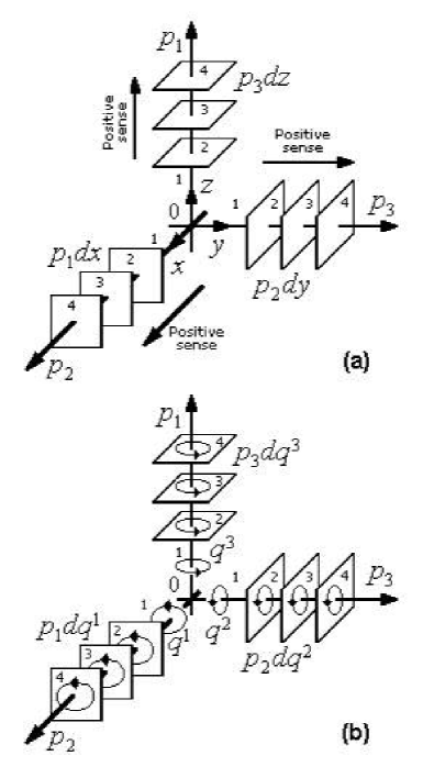
Figure 1: Basis vectors and one-forms in Euclidean $\mathbb{R}^{3}-$space: (a) Translational case; and (b) Rotational case [2]. For the same geometry in $\mathbb{R}^{3}$, see [11].

• any scalar function $f=f(x,y,z)$ is a 0–form;

• the gradient $\mathbf{d}f=\mathbf{\omega}$ of any smooth function $f$ is a 1–form

  $$\mathbf{\omega=d}f=\frac{\partial f}{\partial x}dx+\frac{\partial f}{\partial y}dy+\frac{\partial f}{\partial z}dz;$$

• the curl $\mathbf{\alpha=d\omega}$ of any smooth 1–form $\mathbf{\omega}$ is a 2–form

  $$\mathbf{\alpha=d\omega}=\left(\frac{\partial R}{\partial y}-\frac{\partial Q}{\partial z}\right)dydz+\left(\frac{\partial P}{\partial z}-\frac{\partial R}{\partial x}\right)dzdx+\left(\frac{\partial Q}{\partial x}-\frac{\partial P}{\partial y}\right)dxdy;$$

  $$\text{if }\mathbf{\omega=d}f\Rightarrow\mathbf{\alpha=dd}f=0.$$

• the divergence $\mathbf{\beta=d\alpha}$ of any smooth 2–form $\mathbf{\alpha}$ is a 3–form

  $$\mathbf{\beta=d\alpha}=\left(\frac{\partial A}{\partial x}+\frac{\partial B}{\partial y}+\frac{\partial C}{\partial z}\right)dxdydz;\qquad\text{if }\mathbf{\alpha=d\omega}\Rightarrow\mathbf{\beta=dd\omega}=0.$$

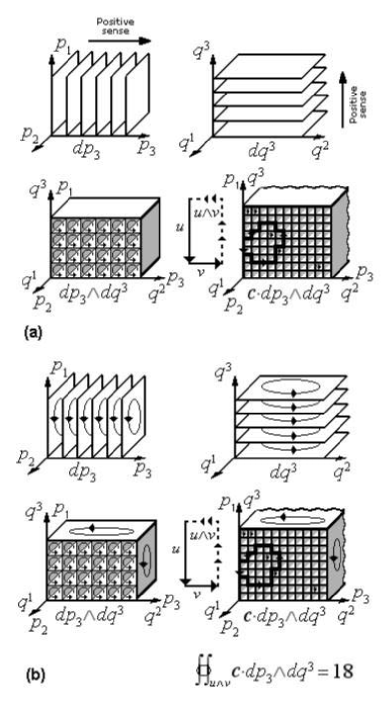
Figure 2: Fundamental two–form and its flux in $\mathbb{R}^{3}$: (a) Translational case; (b) Rotational case. In both cases the flux through the plane $u\wedge v$ is defined as $\int\int_{u\wedge v}c\,dp_{i}dq^{i}$ and measured by the number of tubes crossed by the circulation oriented by $u\wedge v$ [2]. For the same geometry in $\mathbb{R}^{3}$, see [11].

In general, for any two smooth functions $f=f(x,y,z)$ and $g=g(x,y,z)$, the exterior derivative $\mathbf{d}$ obeys the Leibniz rule [3, 4]:

$$\mathbf{d}(fg)=g\,\mathbf{d}f+f\,\mathbf{d}g,$$

and the chain rule:

$$\mathbf{d}\left(g(f)\right)=g^{\prime}(f)\,\mathbf{d}f.$$

1.3 Exterior forms

In general, given a so–called 4D coframe, that is a set of coordinate differentials $\{dx^{i}\}\in\mathbb{R}^{4}$, we can define the space of all $p-$forms, denoted $\Omega^{p}(\mathbb{R}^{4})$, using the exterior derivative $\mathbf{d}:\Omega^{p}(\mathbb{R}^{4})\rightarrow\Omega^{p+1}(\mathbb{R}^{4})$ and Einstein’s summation convention over repeated indices (e.g., $A_{i}\,dx^{i}=\sum_{i=0}^{3}A_{i}\,dx^{i}$), we have:

1–form

– a generalization of the Green’s 1–form $Pdx+Qdy$,

$$\mathbf{A}=A_{i}\,dx^{i}\in\Omega^{1}(\mathbb{R}^{4}).$$

For example, in 4D electrodynamics, $\mathbf{A}$ represents electromagnetic (co)vector potential.

2–form

– generalizing the Green’s 2–form $(\partial_{x}Q-\partial_{y}P)\,dxdy$  $($with $\partial_{j}=\partial/\partial x^{j}$),

$$\mathbf{B} = \mathbf{dA}\in\Omega^{2}(\mathbb{R}^{4}),\qquad\text{with components}$$

$$\mathbf{B} = \frac{1}{2}B_{ij}\,dx^{i}\wedge dx^{j},\qquad\text{or}$$

$$\mathbf{B} = \partial_{j}A_{i}\,dx^{j}\wedge dx^{i},\qquad\text{so that}$$

$$B_{ij} = -2\partial_{j}A_{i}=\partial_{i}A_{j}-\partial_{j}A_{i}=-B_{ji}.$$

where $\wedge$ is the anticommutative exterior (or, ‘wedge’) product of two differential forms; given a $p-$form $\mathbf{\alpha}\in\Omega^{p}(\mathbb{R}^{4})$ and a $q-$form $\mathbf{\beta}\in\Omega^{q}(\mathbb{R}^{4}),$ their exterior product is a $(p+q)-$form $\mathbf{\alpha}\wedge\mathbf{\beta}\in\Omega^{p+q}(\mathbb{R}^{4})$; e.g., if we have two 1–forms $\mathbf{a}=a_{i}dx^{i}$, and $\mathbf{b}=b_{i}dx^{i}$, their wedge product $\mathbf{a}\wedge\mathbf{b}$ is a 2–form $\mathbf{\alpha}$ given by

$$\mathbf{\alpha}=\mathbf{a}\wedge\mathbf{b}=a_{i}b_{j}\,dx^{i}\wedge dx^{j}=-a_{i}b_{j}\,dx^{j}\wedge dx^{i}=-\mathbf{b}\wedge\mathbf{a}.$$

The exterior product $\wedge$ is related to the exterior derivative $\mathbf{d}=\partial_{i}dx^{i}$, by

$$\mathbf{d}(\mathbf{\alpha}\wedge\mathbf{\beta})=\mathbf{d\alpha}\wedge\mathbf{\beta}+(-1)^{p}\mathbf{\alpha}\wedge\mathbf{d\beta}.\text{ \ }$$

3–form

$$\mathbf{C} = \mathbf{dB~{}(}=\mathbf{ddA}\equiv 0)\in\Omega^{3}(\mathbb{R}^{4}),\qquad\text{with components}$$

$$\mathbf{C} = \frac{1}{3!}C_{ijk}\,dx^{i}\wedge dx^{j}\wedge dx^{k},\qquad\text{or}$$

$$\mathbf{C} = \partial_{k}B_{[ij]}\,dx^{k}\wedge dx^{i}\wedge dx^{j},\qquad\text{so that}$$

$$C_{ijk} = -6\partial_{k}B_{[ij]},\qquad\text{where }B_{[ij]}\text{ is the skew--symmetric part of }B_{ij}.$$

For example, in the 4D electrodynamics, $\mathbf{B}$ represents the field 2–form Faraday, or the Liénard–Wiechert 2–form (in the next section we will use the standard symbol $\mathbf{F}$ instead of $\mathbf{B}$) satisfying the sourceless magnetic Maxwell’s equation,

$$\text{Bianchi identity}:\quad\mathbf{dB}=0,\quad\text{in components\quad}\partial_{k}B_{[ij]}=0.$$

4–form

$$\mathbf{D} = \mathbf{dC~{}(}=\mathbf{ddB}\equiv 0)\in\Omega^{4}(\mathbb{R}^{4}),\qquad\text{with components}$$

$$\mathbf{D} = \partial_{l}C_{[ijk]}\,dx^{l}\wedge dx^{i}\wedge dx^{j}\wedge dx^{k},\qquad\text{or}$$

$$\mathbf{D} = \frac{1}{4!}D_{ijkl}\,dx^{i}\wedge dx^{j}\wedge dx^{k}\wedge dx^{l},\qquad\text{so that}$$

$$D_{ijkl} = -24\partial_{l}C_{[ijk]}.$$

1.4 Stokes theorem

Generalization of the Green’s theorem in the plane (and all other integral theorems from vector calculus) is the Stokes theorem for the $p-$form $\mathbf{\omega}$, in an oriented $n$D domain $C$ (which is a $p-$chain with a $(p-1)-$boundary $\partial C$, see next section)

$$\int_{\partial C}\mathbf{\omega}=\int_{C}\mathbf{d\omega}.$$

For example, in the 4D Euclidean space $\mathbb{R}^{4}$ we have the following three particular cases of the Stokes theorem, related to the subspaces $C$ of $\mathbb{R}^{4}$:
The 2D Stokes theorem:

$$\int_{\partial C^{2}}\mathbf{A}=\int_{C^{2}}\mathbf{B}.$$

The 3D Stokes theorem:

$$\int_{\partial C^{3}}\mathbf{B}=\int_{C^{3}}\mathbf{C}.$$

The 4D Stokes theorem:

$$\int_{\partial C^{4}}\mathbf{C}=\int_{C^{4}}\mathbf{D}.$$

2 De Rham–Hodge Theory Basics

Now that we are familiar with differential forms and Stokes’ theorem, we can introduce Hodge–De Rham theory.

2.1 Exact and closed forms and chains

Notation change: we drop boldface letters from now on. In general, a $p-$form $\beta$ is called closed if its exterior derivative $d=\partial_{i}dx^{i}$ is equal to zero,

$$d\beta=0.$$

From this condition one can see that the closed form (the kernel of the exterior derivative operator $d$) is conserved quantity. Therefore, closed $p-$forms possess certain invariant properties, physically corresponding to the conservation laws (see e.g., [6]).

Also, a $p-$form $\beta$ that is an exterior derivative of some $(p-1)-$form $\alpha$,

$$\beta=d\alpha,$$

is called exact (the image of the exterior derivative operator $d$). By Poincaré lemma, exact forms prove to be closed automatically,

$$d\beta=d(d\alpha)=0.$$

Since $d^{2}=0$, every exact form is closed. The converse is only partially true, by Poincaré lemma: every closed form is locally exact.

Technically, this means that given a closed $p-$form $\alpha\in\Omega^{p}(U)$, defined on an open set $U$ of a smooth manifold $M$ (see Figure 3), any point $m\in U$ has a neighborhood on which there exists a $(p-1)-$form $\beta\in\Omega^{p-1}(U)$ such that $d\beta=\alpha|_{U}.$

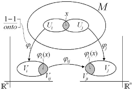
Figure 3: Depicting the manifold concept (see footnote 1).

In particular, there is a Poincaré lemma for contractible manifolds: Any closed form on a smoothly contractible manifold is exact.

The Poincaré lemma is a generalization and unification of two well–known facts in vector calculus:
(i) If $\mathop{\mathrm{c}url}F=0$, then locally $F=\mathop{\mathrm{g}rad}f$;   and   (ii) If $\mathop{\mathrm{d}iv}F=0$, then locally $F=\mathop{\mathrm{c}url}G$.

A cycle is a $p-$chain, (or, an oriented $p-$domain) $C\in\mathcal{C}_{p}(M)$ such that $\partial C=0$. A boundary is a chain $C$ such that $C=\partial B,$ for any other chain $B\in\mathcal{C}_{p}(M)$. Similarly, a cocycle (i.e., a closed form) is a cochain $\omega$ such that $d\omega=0$. A coboundary (i.e., an exact form) is a cochain $\omega$ such that $\omega=d\theta,$ for any other cochain $\theta$. All exact forms are closed ($\omega=d\theta\Rightarrow d\omega=0$) and all boundaries are cycles ($C=\partial B\Rightarrow\partial C=0$). Converse is true only for smooth contractible manifolds, by Poincaré lemma.

2.2 De Rham duality of forms and chains

Integration on a smooth manifold $M$ should be thought of as a nondegenerate bilinear pairing $\left\langle,\right\rangle$ between $p-$forms and $p-$chains (spanning a finite domain on $M$). Duality of $p-$forms and $p-$chains on $M$ is based on the De Rham’s ‘period’, defined as [9, 7]

$$\text{Period}:=\int_{C}\omega:=\left\langle C,\omega\right\rangle,$$

where $C$ is a cycle, $\omega$ is a cocycle, while $\left\langle C,\omega\right\rangle=\omega(C)$ is their inner product $\left\langle C,\omega\right\rangle:\Omega^{p}(M)\times\mathcal{C}_{p}(M)\rightarrow\mathbb{R}$. From the Poincaré lemma, a closed $p-$form $\omega$ is exact iff $\left\langle C,\omega\right\rangle=0$.

The fundamental topological duality is based on the Stokes theorem,

$$\int_{\partial C}\omega=\int_{C}d\omega\qquad\mathrm{or}\qquad\left\langle\partial C,\omega\right\rangle=\left\langle C,d\omega\right\rangle,$$

where $\partial C$ is the boundary of the $p-$chain $C$ oriented coherently with $C$ on $M$. While the boundary operator $\partial$ is a global operator, the coboundary operator $d$ is local, and thus more suitable for applications. The main property of the exterior differential,

$$d\circ d\equiv d^{2}=0\quad\Longrightarrow\quad\partial\circ\partial\equiv\partial^{2}=0,\qquad(\text{and converse}),$$

can be easily proved using the Stokes’ theorem (and the above ‘period notation’) as

$$0=\left\langle\partial^{2}C,\omega\right\rangle=\left\langle\partial C,d\omega\right\rangle=\left\langle C,d^{2}\omega\right\rangle=0.$$

2.3 De Rham cochain and chain complexes

In the Euclidean 3D space $\mathbb{R}^{3}$ we have the following De Rham cochain complex

$$0\rightarrow\Omega^{0}(\mathbb{R}^{3})\underset{\mathrm{grad}}{\overset{d}{\longrightarrow}}\Omega^{1}(\mathbb{R}^{3})\underset{\mathrm{curl}}{\overset{d}{\longrightarrow}}\Omega^{2}(\mathbb{R}^{3})\underset{\mathrm{div}}{\overset{d}{\longrightarrow}}\Omega^{3}(\mathbb{R}^{3})\rightarrow 0.$$

Using the closure property for the exterior differential in $\mathbb{R}^{3},~{}d\circ d\equiv d^{2}=0$, we get the standard identities from vector calculus

$$\mathop{\mathrm{c}url}\cdot\mathop{\mathrm{g}rad}=0\text{ \ \ \ \ \ \ and \ \ \ \ \ \ }\mathop{\mathrm{d}iv}\cdot\mathop{\mathrm{c}url}=0.$$

As a duality, in $\mathbb{R}^{3}$ we have the following chain complex

$$0\leftarrow\mathcal{C}_{0}(\mathbb{R}^{3}){\overset{\partial}{\longleftarrow}}\mathcal{C}_{1}(\mathbb{R}^{3}){\overset{\partial}{\longleftarrow}}\mathcal{C}_{2}(\mathbb{R}^{3}){\overset{\partial}{\longleftarrow}}\mathcal{C}_{3}(\mathbb{R}^{3})\leftarrow 0,$$

(with the closure property $\partial\circ\partial\equiv\partial^{2}=0$) which implies the following three boundaries:

$$C_{1}\overset{\partial}{\mapsto}C_{0}=\partial(C_{1}),\qquad C_{2}\overset{\partial}{\mapsto}C_{1}=\partial(C_{2}),\qquad C_{3}\overset{\partial}{\mapsto}C_{2}=\partial(C_{3}),$$

where $C_{0}\in\mathcal{C}_{0}$ is a 0–boundary (or, a point), $C_{1}\in\mathcal{C}_{1}$ is a 1–boundary (or, a line), $C_{2}\in\mathcal{C}_{2}$ is a 2–boundary (or, a surface), and $C_{3}\in\mathcal{C}_{3}$ is a 3–boundary (or, a hypersurface). Similarly, the De Rham complex implies the following three coboundaries:

$$C^{0}\overset{d}{\mapsto}C^{1}=d(C^{0}),\qquad C^{1}\overset{d}{\mapsto}C^{2}=d(C^{1}),\qquad C^{2}\overset{d}{\mapsto}C^{3}=d(C^{2}),$$

where $C^{0}\in\Omega^{0}$ is 0–form (or, a function), $C^{1}\in\Omega^{1}$ is a 1–form, $C^{2}\in\Omega^{2}$ is a 2–form, and $C^{3}\in\Omega^{3}$ is a 3–form.

In general, on a smooth $n$D manifold $M$ we have the following De Rham cochain complex [9]

$$0\rightarrow\Omega^{0}(M)\overset{d}{\longrightarrow}\Omega^{1}(M)\overset{d}{\longrightarrow}\Omega^{2}(M)\overset{d}{\longrightarrow}\Omega^{3}(M)\overset{d}{\longrightarrow}\cdot\cdot\cdot\overset{d}{\longrightarrow}\Omega^{n}(M)\rightarrow 0,$$

satisfying the closure property on $M,~{}d\circ d\equiv d^{2}=0$.

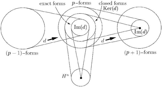
Figure 4: A small portion of the De Rham cochain complex, showing a homomorphism of cohomology groups.

2.4 De Rham cohomology vs. chain homology

Briefly, the De Rham cohomology is the (functional) space of closed differential $p-$forms modulo exact ones on a smooth manifold.

More precisely, the subspace of all closed $p-$forms (cocycles) on a smooth manifold $M$ is the kernel $\mathop{\mathrm{K}er}(d)$ of the De Rham $d-$homomorphism (see Figure 4), denoted by $Z^{p}(M)\subset\Omega^{p}(M)$, and the sub-subspace of all exact $p-$forms (coboundaries) on $M$ is the image $\mathop{\mathrm{I}m}(d)$ of the De Rham homomorphism denoted by $B^{p}(M)\subset Z^{p}(M)$. The quotient space

$$H^{p}_{DR}(M):=\frac{Z^{p}(M)}{B^{p}{M}}=\frac{\mathop{\mathrm{K}er}\left(d:\Omega^{p}(M)\rightarrow\Omega^{p+1}(M)\right)}{\mathop{\mathrm{I}m}\left(d:\Omega^{p-1}(M)\rightarrow\Omega^{p}(M)\right)},$$ (1)

is called the $p$th De Rham cohomology group of a manifold $M$. It is a topological invariant of a manifold. Two $p-$cocycles $\alpha$,$\beta\in\Omega^{p}(M)$ are cohomologous, or belong to the same cohomology class $[\alpha]\in H^{p}(M)$, if they differ by a $(p-1)-$coboundary $\alpha-\beta=d\theta\in\Omega^{p-1}(M)$. The dimension $b_{p}=\dim H^{p}(M)$ of the De Rham cohomology group $H^{p}_{DR}(M)$ of the manifold $M$ is called the Betti number $b_{p}$.

Similarly, the subspace of all $p-$cycles on a smooth manifold $M$ is the kernel $\mathop{\mathrm{K}er}(\partial)$ of the $\partial-$homomorphism, denoted by $Z_{p}(M)\subset\mathcal{C}_{p}(M)$, and the sub-subspace of all $p-$boundaries on $M$ is the image $\mathop{\mathrm{I}m}(\partial)$ of the $\partial-$homomorphism, denoted by $B_{p}(M)\subset\mathcal{C}_{p}(M)$. Two $p-$cycles $C_{1}$,$C_{2}\in\mathcal{C}_{p}$ are homologous, if they differ by a $(p-1)-$boundary $C_{1}-C_{2}=\partial B\in\mathcal{C}_{p-1}(M)$. Then $C_{1}$ and $C_{2}$ belong to the same homology class $[C]\in H_{p}(M)$, where $H_{p}(M)$ is the homology group of the manifold $M$, defined as

$$H_{p}(M):=\frac{Z_{p}(M)}{B_{p}(M)}=\frac{\mathop{\mathrm{K}er}(\partial:\mathcal{C}_{p}(M)\rightarrow\mathcal{C}_{p-1}(M))}{\mathop{\mathrm{I}m}(\partial:\mathcal{C}_{p+1}(M)\rightarrow\mathcal{C}_{p}(M))},$$

where $Z_{p}$ is the vector space of cycles and $B_{p}\subset Z_{p}$ is the vector space of boundaries on $M$. The dimension $b_{p}=\dim H_{p}(M)$ of the homology group $H_{p}(M)$ is, by the De Rham theorem, the same Betti number $b_{p}$.

If we know the Betti numbers for all (co)homology groups of the manifold $M$, we can calculate the Euler–Poincaré characteristic of $M$ as

$$\chi(M)=\sum_{p=1}^{n}(-1)^{p}b_{p}.$$

For example, consider a small portion of the De Rham cochain complex of Figure 4 spanning a space-time 4–manifold $M$,

$$\Omega^{p-1}(M)\overset{d_{p-1}}{\longrightarrow}\Omega^{p}(M)\overset{d_{p}}{\longrightarrow}\Omega^{p+1}(M)$$

As we have seen above, cohomology classifies topological spaces by comparing two subspaces of  $\Omega^{p}$:  (i) the space of $p-$cocycles, $Z^{p}(M)=\mathop{\mathrm{K}er}d_{p}$, and  (ii) the space of $p-$coboundaries, $B^{p}(M)=\mathop{\mathrm{I}m}d_{p-1}$. Thus, for the cochain complex of any space-time 4–manifold we have,

$$d^{2}=0\quad\Rightarrow\quad B^{p}(M)\subset Z^{p}(M),$$

that is, every $p-$coboundary is a $p-$cocycle. Whether the converse of this statement is true, according to Poincaré lemma, depends on the particular topology of a space-time 4–manifold. If every $p-$cocycle is a $p-$coboundary, so that $B^{p}$ and $Z^{p}$ are equal, then the cochain complex is exact at $\Omega^{p}(M)$. In topologically interesting regions of a space-time manifold $M$, exactness may fail [13], and we measure the failure of exactness by taking the $p$th cohomology group

$$H^{p}(M)=Z^{p}(M)/B^{p}(M).$$

2.5 Hodge star operator

The Hodge star operator $\star:\Omega^{p}(M)\rightarrow\Omega^{n-p}(M)$, which maps any $p-$form $\alpha$ into its dual $(n-p)-$form $\star\,\alpha$ on a smooth $n-$manifold $M$, is defined as (see, e.g. [8])

$$\alpha\wedge\star\,\beta=\beta\wedge\star\,\alpha=\left\langle\alpha,\beta\right\rangle\mu,\qquad\text{for }\alpha,\beta\in\Omega^{p}(M),$$

$$\star\star\alpha=(-1)^{p(n-p)}\alpha,$$

$$\star\,(c_{1}\alpha+c_{2}\beta)=c_{1}(\star\,\alpha)+c_{2}(\star\,\beta),$$

$$\alpha\wedge\star\,\alpha=0\Rightarrow\alpha\equiv 0.$$

The $\star$ operator depends on the Riemannian metric $g=g_{ij}$ on $M$ and also on the orientation (reversing orientation will change the sign) [4]. The volume form $\mu$ is defined in local coordinates on an $n-$manifold $M$ as (compare with Hodge inner product below)

$$\mu=\text{vol}=\star\,(1)=\sqrt{\det(g_{ij})}~{}dx^{1}\wedge...\wedge dx^{n},$$ (2)

and the total volume on $M$ is given by

$$\mathop{\mathrm{v}ol}(M)=\int_{M}\star\,(1).$$

For example, in Euclidean $\mathbb{R}^{3}$ space with Cartesian $(x,y,z)$ coordinates, we have:

$$\star\,dx=dy\wedge dz,\qquad\star\,dy=dz\wedge dx,\qquad\star\,dz=dx\wedge dy.$$

The Hodge dual in this case clearly corresponds to the 3D cross–product.

In the 4D–electrodynamics, the dual 2–form Maxwell $\star\,F$ satisfies the electric Maxwell equation with the source [11],

$$\text{Dual Bianchi identity}:\quad{d}\,{\star\,F}=\star\,J,$$

where ${\star\,J}$ is the 3–form dual to the charge–current 1–form ${J}$.

2.6 Hodge inner product

For any two $p-$forms $\alpha,\beta\in\Omega^{p}(M)$ with compact support on an $n-$manifold $M$, we define bilinear and positive–definite Hodge $L^{2}-$inner product as

$$(\alpha,\beta)=\int_{M}\langle\alpha,\beta\rangle\star(1)=\int_{M}\alpha\wedge\star\,\beta,$$ (3)

where $\alpha\wedge\star\,\beta$ is an $n-$form. We can extend the product $(\cdot,\cdot)$ to $L^{2}(\Omega^{p}(M))$; it remains bilinear and positive–definite, because as usual in the definition of $L^{2}$, functions that differ only on a set of measure zero are identified. The inner product (3) is evidently linear in each variable and symmetric, $(\alpha,\beta)=(\beta,\alpha)$. We have: $(\alpha,\alpha)\geq 0$ and $(\alpha,\alpha)=0$ iff $\alpha=0$. Also, $(\star\,\alpha,\star\,\beta)=(\alpha,\beta)$. Thus, operation (3) turns the space $\Omega^{p}(M)$ into an infinite–dimensional inner–product space.

From (3) it follows that for every $p-$form $\alpha\in\Omega^{p}(M)$ we can define the norm functional

$$\left\|\alpha\right\|^{2}=(\alpha,\alpha)=\int_{M}\langle\alpha,\alpha\rangle\star(1)=\int_{M}\alpha\wedge\star\,\alpha,$$

for which the Euler–Lagrangian equation becomes the Laplace equation (see Hodge Laplacian below),

$$\Delta\alpha=0.$$

For example, the standard Lagrangian for the free Maxwell electromagnetic field,
$F=dA$ (where $A=A_{i}dx^{i}$ is the electromagnetic potential 1–form), is given by [3, 4, 5]

$$\mathcal{L}(A)=\frac{1}{2}(F\wedge\star\,F),$$

with the corresponding action

$$S(A)=\frac{1}{2}\int F\wedge\star\,F.$$

Using the Hodge $L^{2}-$inner product (3), we can rewrite this electrodynamic action as

$$S(A)=\frac{1}{2}(F,F).$$ (4)

2.7 Hodge codifferential operator

The Hodge dual (or, formal adjoint) to the exterior derivative $d:\Omega^{p}(M)\rightarrow\Omega^{p+1}(M)$ on a smooth manifold $M$ is the codifferential $\delta$, a linear map $\delta:\Omega^{p}(M)\rightarrow\Omega^{p-1}(M)$, which is a generalization of the divergence, defined by [9, 8]

$$\delta=(-1)^{n(p+1)+1}\star d\,\star,\qquad\text{so that\qquad}d=(-1)^{np}\star\delta\star.$$

That is, if the dimension $n$ of the manifold $M$ is even, then $\delta=-\star d\,\star$.

Applied to any $p-$form $\omega\in\Omega^{p}(M)$, the codifferential $\delta$ gives

$$\delta\omega=(-1)^{n(p+1)+1}\star d\star\omega,\qquad\delta d\omega=(-1)^{np+1}\star d\star d\omega.$$

If $\omega=f$ is a $0-$form, or function, then $\delta f=0$. If a $p-$form $\alpha$ is a codifferential of a $(p+1)-$form $\beta$, that is $\alpha=\delta\beta$, then $\beta$ is called the coexact form. A $p-$form $\alpha$ is coclosed if $\delta\alpha=0$; then $\star\,\alpha$ is closed (i.e., $d\star\alpha=0$) and conversely.

The Hodge codifferential $\delta$ satisfies the following set of rules:

• $\delta\delta=\delta^{2}=0,$  the same as $\ dd=d^{2}=0;$

• $\delta\star=(-1)^{p+1}\star d$;  $\star\,\delta=(-1)^{p}\star d$;

• $d\delta\star=\star\,\delta d$;  $\star\,d\delta=\delta d\star$.

Standard example is classical electrodynamics, in which the gauge field is an electromagnetic potential 1–form (a connection on a $U(1)-$bundle),

$$A=A_{\mu}dx^{\mu}=A_{\mu}dx^{\mu}+df,\qquad(f=~{}\text{arbitrary scalar field}),$$

with the corresponding electromagnetic field 2–form (the curvature of the connection $A$)

$$F = dA,\qquad\text{in components given by}$$

$$F = \frac{1}{2}F_{\mu\nu}\,dx^{\mu}\wedge dx^{\nu},\qquad\text{with \ \ \ }F_{\mu\nu}=\partial_{\nu}A_{\mu}-\partial_{\mu}A_{\nu}.$$

Electrodynamics is governed by the Maxwell equations, which in exterior formulation read

$$dF = 0,\qquad\delta F=-4\pi J,\qquad\text{or in components,}$$

$$F_{[\mu\nu,\eta]} = 0,\qquad F_{\mu\nu},^{\mu}=-4\pi J_{\mu},$$

where comma denotes the partial derivative and the 1–form of electric current $J=J_{\mu}dx^{\mu}$ is conserved, by the electrical continuity equation,

$$\delta J=0,\qquad\text{or in components,\qquad}J_{\mu},^{\mu}=0.$$

2.8 Hodge Laplacian operator

The codifferential $\delta$ can be coupled with the exterior derivative $d$ to construct the Hodge Laplacian $\Delta:$ $\Omega^{p}(M)\rightarrow\Omega^{p}(M),$ a harmonic generalization of the Laplace–Beltrami differential operator, given by

$$\Delta=\delta d+d\delta=(d+\delta)^{2}.$$

$\Delta$ satisfies the following set of rules:

$$\delta\,\Delta=\Delta\,\delta=\delta d\delta;\qquad d\,\Delta=\Delta\,d=d\delta d;\qquad\star\;\Delta=\Delta\star.$$

A $p-$form $\alpha$ is called harmonic iff

$$\Delta\alpha=0~{}\Leftrightarrow~{}(d\alpha=0,\delta\alpha=0).$$

Thus, $\alpha$ is harmonic in a compact domain $D\subset M$ iff it is both closed and coclosed in $D$. Informally, every harmonic form is both closed and coclosed. As a proof, we have:

$$0=\left(\alpha,~{}\Delta\alpha\right)=\left(\alpha,d\delta\alpha\right)+\left(\alpha,\delta d\alpha\right)=\left(\delta\alpha,\delta\alpha\right)+\left(d\alpha,d\alpha\right).$$

Since $\left(\beta,~{}\beta\right)\geq 0$ for any form $\beta$, $\left(\delta\alpha,\delta\alpha\right)$ and $\left(d\alpha,d\alpha\right)$ must vanish separately. Thus, $d\alpha=0$ and $\delta\alpha=0.$

All harmonic $p-$forms on a smooth manifold $M$ form the vector space $H^{p}_{\Delta}(M)$.

Also, given a $p-$form $\lambda,$ there is another $p-$form $\eta$ such that the equation

$$\Delta\eta=\lambda$$

is satisfied iff for any harmonic $p-$form $\gamma$ we have $\ (\gamma,\lambda)=0.$

For example, to translate notions from standard 3D vector calculus, we first identify scalar functions with 0–forms, field intensity vectors with 1–forms, flux vectors with 2–forms and scalar densities with 3–forms. We then have the following correspondence:

grad $\longrightarrow$ $d$ :  on 0–forms;      curl $\longrightarrow$ $\star\,d$ :  on 1–forms;

div $\longrightarrow$ $\delta$ :  on 1–forms;        div grad $\longrightarrow$ $\Delta$ :  on 0–forms;

curl curl $-$ grad div $\longrightarrow\Delta$ :  on 1–forms.

We remark here that exact and coexact $p-$forms ($\alpha=d\beta$ and $\omega=\delta\beta$) are mutually orthogonal with respect to the $L^{2}-$inner product (3). The orthogonal complement consists of forms that are both closed and coclosed: that is, of harmonic forms ($\Delta\gamma=0$).

2.9 Hodge adjoints and self–adjoints

If $\alpha$ is a $p-$form and $\beta$ is a $(p+1)-$form then we have [9]

$$(d\alpha,\beta)=(\alpha,\delta\beta)\qquad\mathrm{and}\qquad(\delta\alpha,\beta)=(\alpha,d\beta).$$ (5)

This relation is usually interpreted as saying that the two exterior differentials, $d$ and $\delta\,,$ are adjoint (or, dual) to each other. This identity follows from the fact that for the volume form $\mu$ given by (2) we have $d\mu=0$ and thus

$$\int_{M}d(\alpha\wedge\star\beta)=0.$$

Relation (5) also implies that the Hodge Laplacian $\Delta$ is self–adjoint (or, self–dual),

$$(\Delta\alpha,\beta)=(\alpha,\Delta\beta),$$

which is obvious as either side is $(d\alpha,d\beta)+(\delta\alpha,\delta\beta).$ Since $(\Delta\alpha,\alpha)\geq 0,$ with $(\Delta\alpha,\alpha)=0$ only when $\Delta\alpha=0,$ $\Delta$ is a positive–definite (elliptic) self–adjoint differential operator.

2.10 Hodge decomposition theorem

The celebrated Hodge decomposition theorem (HDT) states that, on a compact orientable smooth $n-$manifold $M$ (with $n\geq p$), any exterior $p-$form can be written as a unique sum of an exact form, a coexact form, and a harmonic form. More precisely, for any form $\omega\in\Omega^{p}(M)$ there are unique forms $\alpha\in\Omega^{p-1}(M),$ $\beta\in\Omega^{p+1}(M)$ and a harmonic form $\gamma\in\Omega^{p}(M),$ such that

$${\mathrm{H}DT:}\qquad\stackrel{{\scriptstyle\mathrm{a}ny\,form}}{{\omega}}\quad=\quad\stackrel{{\scriptstyle\mathrm{e}xact}}{{d\alpha}}\quad+\quad\stackrel{{\scriptstyle\mathrm{c}oexact}}{{\delta\beta}}\quad+\quad\stackrel{{\scriptstyle\mathrm{h}armonic}}{{\gamma}}$$

For the proof, see [8, 9].

In physics community, the exact form $d\alpha$ is called longitudinal, while the coexact form $\delta\beta$ is called transversal, so that they are mutually orthogonal. Thus any form can be orthogonally decomposed into a harmonic, a longitudinal and transversal form. For example, in fluid dynamics, any vector-field $v$ can be decomposed into the sum of two vector-fields, one of which is divergence–free, and the other is curl–free.

Since $\gamma$ is harmonic, $d\gamma=0.$ Also, by Poincaré lemma, $d(d\alpha)=0.$ In case $\omega$ is a closed $p-$form, $d\omega=0,$ then the term $\delta\beta$ in HDT is absent, so we have the short Hodge decomposition,

$$\omega=d\alpha+\gamma,$$ (6)

thus $\omega$ and $\gamma$ differ by $d\alpha$. In topological terminology, $\omega$ and $\gamma$ belong to the same cohomology class $[\omega]\in H^{p}(M)$. Now, by the De Rham theorems it follows that if $C$ is any $p-$cycle, then

$$\int_{C}\omega=\int_{C}\gamma,$$

that is, $\gamma$ and $\omega$ have the same periods. More precisely, if $\omega$ is any closed $p-$form, then there exists a unique harmonic $p-$form $\gamma$ with the same periods as those of $\omega$ (see [9, 10]).

The Hodge–Weyl theorem [8, 9] states that every De Rham cohomology class has a unique harmonic representative. In other words, the space $H^{p}_{\Delta}(M)$ of harmonic $p-$forms on a smooth manifold $M$ is isomorphic to the De Rham cohomology group (1), or
$H^{p}_{\Delta}(M)\cong H^{p}_{DR}(M)$. That is, the harmonic part $\gamma$ of HDT depends only on the global structure, i.e., the topology of $M$.

For example, in $(2+1)$D electrodynamics, $p-$form Maxwell equations in the Fourier domain $\Sigma$ are written as [15]

$$\begin{array}[]{ll}dE=i\omega B,&\qquad dB=0,\\ dH=-i\omega D+J,&\qquad dD=Q,\end{array}$$

where $H$ is a 0–form (magnetizing field), $D$ (electric displacement field), $J$ (electric current density) and $E$ (electric field) are 1–forms, while $B$ (magnetic field) and $Q$ (electric charge density) are 2–forms. From $d^{2}=0$ it follows that the $J$ and the $Q$ satisfy the continuity equation

$$dJ=iwQ,$$

where $i=\sqrt{-1}$ and $w$ is the field frequency. Constitutive equations, which include all metric information in this framework, are written in terms of Hodge star operators (that fix an isomorphism between $p$ forms and $(2-p)$ forms in the $(2+1)$ case)

$$D=\star\,E,\qquad B=\star\,H.$$

Applying HDT to the electric field intensity 1–form $E$, we get [16]

$$E=d\phi+\delta A+\chi,$$

where $\phi$ is a 0–form (a scalar field) and $A$ is a 2–form; $d\phi$ represents the static field and $\delta A$ represents the dynamic field, and $\chi$ represents the harmonic field component. If domain $\Sigma$ is contractible, $\chi$ is identically zero and we have the short Hodge decomposition,

$$E=d\phi+\delta A.$$

3 Hodge Decomposition and Gauge Path Integral

3.1 Feynman Path Integral

The ‘driving engine’ of quantum field theory is the Feynman path integral. Very briefly, there are three basic forms of the path integral (see, e.g., [5]):

1. Sum–over–histories, developed in Feynman’s version of quantum mechanics (QM) [17];

2. Sum–over–fields, started in Feynman’s version of quantum electrodynamics (QED) [18] and later improved by Fadeev–Popov [20];

3. Sum–over–geometries/topologies in quantum gravity (QG), initiated by S. Hawking and properly developed in the form of causal dynamical triangulations (see [21]; for a ‘softer’ review, see [22]).

In all three versions, Feynman’s action–amplitude formalism includes two components:

1. A real–valued, classical, Hamilton’s action functional,

$$S[\Phi]~{}:=~{}\int_{t_{ini}}^{t_{fin}}{L}[\Phi]\,dt,$$

with the Lagrangian energy function defined over the Lagrangian density $\mathcal{L}$,

$${L}[\Phi]=\int d^{n}x\,\mathcal{L}(\Phi,\partial_{\mu}\Phi),\qquad(\partial_{\mu}\equiv\partial/\partial x^{\mu}),$$

while $\Phi$ is a common symbol denoting all three things to be summed upon (histories, fields and geometries). The action functional $S[\Phi]$ obeys the Hamilton’s least action principle,  $\delta S[\Phi]=0,$  and gives, using standard variational methods, the Euler–Lagrangian equations, which define the shortest path, the extreme field, and the geometry of minimal curvature (and without holes).

2. A complex–valued, quantum transition amplitude,

$$\langle\mathrm{Out}_{t_{fin}}|\mathrm{In}_{t_{ini}}\rangle~{}:=\int_{\mathrm{\Omega}}\mathcal{D}[\Phi]\,\mathrm{e}^{\mathrm{i}S[\Phi]},$$ (11)

where $\mathcal{D}[\Phi]$ is ‘an appropriate’ Lebesgue–type measure,

$$\mathcal{D}[\Phi]=\lim_{N\rightarrow\infty}\prod_{s=1}^{N}\Phi_{s}^{i},\qquad(i=1,...,n),$$

so that we can ‘safely integrate over a continuous spectrum and sum over a discrete spectrum of our problem domain $\Omega$’, of which the absolute square is the real–valued probability density function,

$$P~{}:=~{}|\langle\mathrm{Out}_{t_{fin}}|\mathrm{In}_{t_{ini}}\rangle\rangle|^{2}.$$

This procedure can be redefined in a mathematically cleaner way if we Wick–rotate the time variable $t$ to imaginary values, $t\mapsto\tau={}t$, thereby making all integrals real:

$$\int\mathcal{D}[\Phi]\,\mathrm{e}^{\mathrm{i}S[\Phi]}~{}{\makebox[42.00003pt]{\rule[-1.49994pt]{0.0pt}{16.94444pt}\raisebox{1.50009pt}{\begin{picture}(4.2,0.4)(-0.3,-0.2)\put(1.8,0.2){\makebox(0.0,0.0)[b]{$Wick$}}\put(0.0,0.0){\vector(1,0){3.6}}\end{picture}}}}\quad\int\mathcal{D}[\Phi]\,\mathrm{e}^{-S[\Phi]}.$$ (12)

For example, in non-relativistic quantum mechanics (see Appendix), the propagation amplitude from $x_{a}$ to $x_{b}$ is given by the configuration path integral

$$U(x_{a},x_{b};T)=\left\langle x_{b}|x_{a}\right\rangle=\left\langle x_{b}|\,\mathrm{e}^{-\mathrm{i}HT}|x_{a}\right\rangle=\int\mathcal{D}[x(t)]\,\mathrm{e}^{\mathrm{i}S[x(t)]},$$

which satisfies the Schrödinger equation (in natural units)

$$i\frac{\partial}{\partial T}U(x_{a},x_{b};T)=\hat{H}U(x_{a},x_{b};T),\qquad\text{where \ \ \ \ \ }\hat{H}=-\frac{1}{2}\frac{\partial^{2}}{\partial x_{b}^{2}}+V(x_{b}).$$

3.1.1 Functional measure on the space of differential forms

The Hodge inner product (3) leads to a natural (metric–dependent) functional measure $\mathcal{D}\mu[\omega]$ on $\Omega^{p}(M)$, which normalizes the Gaussian functional integral

$$\int\mathcal{D}\mu[\omega]\,\mathrm{e}^{\mathrm{i}\langle\omega|\omega\rangle}=1.$$ (13)

One can use the invariance of (13) to determine how the functional measure transforms under the Hodge decomposition. Using HDT and its orthogonality with respect to the inner product (3), it was shown in [23] that

$$\langle\omega,\omega\rangle=\langle\gamma,\gamma\rangle+\langle d\alpha,d\alpha\rangle+\langle\delta\beta,\delta\beta\rangle=\langle\gamma,\gamma\rangle+\langle\alpha,\delta d\alpha\rangle+\langle\beta,d\delta\beta\rangle\,,$$ (14)

where the following differential/conferential identities were used [24]

$$\langle d\alpha,d\alpha\rangle=\langle\alpha,\delta d\alpha\rangle\qquad\text{and\qquad}\langle\delta\beta,\delta\beta\rangle=\langle\beta,d\delta\beta\rangle.$$

Since, for any linear operator $O$, one has

$$\int\mathcal{D}\mu[\omega]\exp\mathrm{i}\langle\omega|O\omega\rangle={\det}^{-1/2}(O),$$

(13) and (14) imply that

$$\mathcal{D}\mu[\omega]=\mathcal{D}\mu[\gamma]\mathcal{D}\mu[\alpha]\mathcal{D}\mu[\beta]\,{\det}^{1/2}(\delta d){\det}^{1/2}(d\delta).$$

3.1.2 Abelian Chern–Simons theory

Recall that the classical action for an Abelian Chern–Simons theory,

$$S=\int_{M}A\wedge dA\,,$$

is invariant (up to a total divergence) under the gauge transformation:

$$A\longmapsto A+d\varphi.$$ (15)

We wish to compute the partition function for the theory

$$Z:=\int\frac{1}{V_{G}}\mathcal{D}\mu[A]\,\mathrm{e}^{\mathrm{i}S[A]},$$

where $V_{G}$ denotes the volume of the group of gauge transformations in (15), which must be factored out of the partition function in order to guarantee that the integration is performed only over physically distinct gauge fields. We can handle this by using the Hodge decomposition to parametrize the potential $A$ in terms of its gauge invariant, and gauge dependent parts, so that the volume of the group of gauge transformations can be explicitly factored out, leaving a functional integral over gauge invariant modes only [23].

We now transform the integration variables:

$$A\longmapsto\alpha,\beta,\gamma,$$

where $\alpha,\beta,\gamma$ parameterize respectively the exact, coexact, and harmonic parts of the connection A. Using the Jacobian (14) as well as the following identity on 0–forms $\Delta=\delta d,$ we get [23]

$$Z=\int\frac{1}{V_{G}}\mathcal{D}\mu[\alpha]\mathcal{D}\mu[\beta]\mathcal{D}\mu[\gamma]\,{\det}^{1/2}\left(\Delta\right){\det}^{1/2}\left(d\delta\right)\mathrm{e}^{\mathrm{i}S},$$

from which it follows that

$$V_{G}=\int\mathcal{D}\mu[\alpha],$$ (16)

while the classical action functional becomes, after integrating by parts, using the harmonic properties of $\gamma$ and the nilpotency of the exterior derivative operators, and dropping surface terms:

$$S=-\langle\beta,\star\delta d\delta\beta\rangle\,\,.$$

Note that $S$ depends only the coexact (transverse) part of $A$. Using (16) and integrating over $\beta$ yields:

$$Z=\int\mathcal{D}\mu[\gamma]{\det}^{-1/2}\left(\star\delta d\delta\right){\det}^{1/2}\left(\Delta\right){\det}^{1/2}\left(d\delta\right).$$

Also, it was proven in [23] that

$${\det}(\star\delta d\delta)={\det}^{1/2}((d\delta d)(\delta d\delta))={\det}^{\frac{3}{2}}(d\delta).$$

As a consequence of Hodge duality we have the identity

$${\det}(\delta d)={\det}(d\delta),$$

from which it follows that

$$Z=\int\mathcal{D}\mu[\gamma]\,{\det}^{-3/4}\left(\Delta_{(1)}^{T}\right){\det}^{1/2}\left(\Delta\right){\det}^{1/2}\left(\Delta_{(1)}^{T}\right)\,.$$

The operator $\Delta_{(1)}^{T}$ is the transverse part of the Hodge Laplacian acting on $1-$forms:

$$\Delta_{(1)}^{T}:=(\delta d)_{(1)}.$$

Applying identity for the Hodge Laplacian $\Delta_{(p)}$ [23]

$$\det\left(\Delta_{(p)}\right)=\det\left((\delta d)_{(p)}\right)\det\left((\delta d)_{(p-1)}\right),$$

we get

$${\det}\left(\Delta_{(1)}^{T}\right)={\det}\left(\Delta_{(1)}\right)/{\det}\left(\Delta\right)$$

and hence

$$Z=\int\mathcal{D}\mu[\gamma]\,{\det}^{-1/4}\left(\Delta_{(1)}\right){\det}^{3/4}\left(\Delta\right).$$

The space of harmonic forms $\gamma$ (of any order) is a finite set. Hence, the integration over harmonic forms (3.1.2) is a simple sum.

3.2 Appendix: Path Integral in Quantum Mechanics

The amplitude $\langle q_{F}|\mathrm{e}^{-\mathrm{i}HT}|q_{I}\rangle$ of a quantum-mechanical system (in natural units $\hbar=c=1$) with Hamiltonian $H$ to propagate from a point $q_{I}$ to a point $q_{F}$ in time $T$ is governed by the unitary operator $\mathrm{e}^{-\mathrm{i}HT}$, or more completely, by the complex Lorentzian path integral (in real time):

$$\langle q_{F}|\mathrm{e}^{-\mathrm{i}HT}|q_{I}\rangle=\int\mathcal{D}\left[q(t)\right]\mathrm{e}^{\mathrm{i}\int_{0}^{T}dtL(\dot{q},q)}.$$ (17)

For example, a quantum particle in a potential $V(q)$ has the Hamiltonian operator:
$\hat{H}=\hat{p}^{2}/2m+V(\hat{q})$, with the corresponding Lagrangian: $L=\frac{1}{2}m\dot{q}^{2}-V(q)$, so the path integral reads:

$$\langle q_{F}|\mathrm{e}^{-\mathrm{i}HT}|q_{I}\rangle=\int\mathcal{D}\left[q(t)\right]\mathrm{e}^{\mathrm{i}\int_{0}^{T}dt[\frac{1}{2}m\dot{q}^{2}-V(q)]}.$$

It is somewhat more rigorous to perform a so-called Wick rotation to Euclidean time, which means substituting $t\rightarrow-\mathrm{i}t$ and rotating the integration contour in the complex $t-$plane, so that we obtain the real path integral in complex time:

$$\langle q_{F}|\mathrm{e}^{-\mathrm{i}HT}|q_{I}\rangle=\int\mathcal{D}\left[q(t)\right]\mathrm{e}^{\mathrm{-}\int_{0}^{T}dtL(\dot{q},q)}=\int\mathcal{D}\left[q(t)\right]\mathrm{e}^{\mathrm{-}(\mathrm{i}/\hbar)\int_{0}^{T}dt[\frac{1}{2}m\dot{q}^{2}-V(q)]},$$

known as the Euclidean path integral.

One particularly nice feature of the path-integral formalism is that the classical limit of quantum mechanics can be recovered easily. We simply restore Planck’s constant $\hbar$ in (17)

$$\langle q_{F}|\mathrm{e}^{-(\mathrm{i}/\hbar)HT}|q_{I}\rangle=\int\mathcal{D}\left[q(t)\right]\mathrm{e}^{(\mathrm{i}/\hbar)\int_{0}^{T}dtL(\dot{q},q)},$$

and take the $\hbar\rightarrow 0$ limit. Applying the stationary phase method (or steepest descent) , see [25]), we obtain $\mathrm{e}^{(\mathrm{i}/\hbar)\int_{0}^{T}dtL(\dot{q}_{c},q_{c})}$, where $q_{c}(t)$ is the recovered classical path determined by solving the Euler-Lagrangian equation: $(d/dt)(\delta L/\delta q)-(\delta L/\delta q)=0,$ with appropriate boundary conditions.

References

- [1] J.E. Marsden, A. Tromba, Vector Calculus (5th ed.), W. Freeman and Company, New York, (2003)
- [2] V. Ivancevic, Symplectic Rotational Geometry in Human Biomechanics, SIAM Rev. 46, 3, 455–474, (2004).
- [3] V. Ivancevic, T. Ivancevic, Geometrical Dynamics of Complex Systems. Springer, Dordrecht, (2006).
- [4] V. Ivancevic, T. Ivancevic, Applied Differfential Geometry: A Modern Introduction. World Scientific, Singapore, (2007)
- [5] V. Ivancevic, T. Ivancevic, Quantum Leap: From Dirac and Feynman, Across the Universe, to Human Body and Mind. World Scientific, Singapore, (2008)
- [6] R. Abraham, J. Marsden, T. Ratiu, Manifolds, Tensor Analysis and Applications. Springer, New York, (1988).
- [7] Y. Choquet-Bruhat, C. DeWitt-Morete, Analysis, Manifolds and Physics (2nd ed). North-Holland, Amsterdam, (1982).
- [8] C. Voisin, Hodge Theory and Complex Algebraic Geometry I. Cambridge Univ. Press, Cambridge, (2002).
- [9] G. de Rham, Differentiable Manifolds. Springer, Berlin, (1984).
- [10] H. Flanders, Differential Forms: with Applications to the Physical Sciences. Acad. Press, (1963).
- [11] C.W. Misner, K.S. Thorne, J.A. Wheeler, Gravitation. W. Freeman and Company, New York, (1973).
- [12] I. Ciufolini, J.A. Wheeler, Gravitation and Inertia, Princeton Series in Physics, Princeton University Press, Princeton, New Jersey, (1995).
- [13] D.K. Wise, p-form electrodynamics on discrete spacetimes. Class. Quantum Grav. 23, 5129–5176, (2006).
- [14] E. Witten, Supersymmetry and Morse theory. J. Diff. Geom., 17, 661–692, (1982).
- [15] F.L. Teixeira and W.C. Chew, Lattice electromagnetic theory from a topological viewpoint, J. Math. Phys. 40, 169–187, (1999).
- [16] B. He, F.L. Teixeira, On the degrees of freedom of lattice electrodynamics. Phys. Let. A 336, 1–7, (2005).
-
[17]
R.P. Feynman, Space–time approach to non–relativistic
quantum mechanics, Rev. Mod. Phys. 20, 367–387, 1948;
R.P. Feynman and A.R. Hibbs, Quantum Mechanics and Path Integrals, McGraw–Hill, New York, 1965. -
[18]
R.P. Feynman, Space–time approach to quantum
electrodynamics, Phys. Rev. 76, 769–789, 1949;
Ibid. Mathematical formulation of the quantum theory of electromagnetic interaction, Phys. Rev. 80, 440–457, 1950. -
[19]
B. Thaller, Visual Quantum Mechanics, Springer, 1999;
Ibid. Advanced Visual Quantum Mechanics, Springer, 2005. - [20] L.D. Faddeev and V.N. Popov, Feynman diagrams for the Yang–Mills field. Phys. Lett. B 25, 29, 1967.
-
[21]
J. Ambjorn, R. Loll, Y. Watabiki, W. Westra and S. Zohren,
A matrix model for 2D quantum gravity defined by Causal Dynamical
Triangulations, Phys.Lett. B 665, 252–256, 2008.;
Ibid. Topology change in causal quantum gravity, Proc. JGRG 17, Nagoya, Japan, December 2007;
Ibid. A string field theory based on Causal Dynamical Triangulations, JHEP 0805, 032, 2008. -
[22]
R. Loll, The emergence of spacetime or quantum gravity on
your desktop, Class. Quantum Grav. 25, 114006, 2008;
R. Loll, J. Ambjorn and J. Jurkiewicz, The Universe from scratch, Contemp. Phys. 47, 103–117, 2006;
J. Ambjorn, J. Jurkiewicz and R. Loll, Reconstructing the Universe, Phys. Rev. D 72, 064014, 2005. - [23] J. Gegenberg, G. Kunstatter, The Partition Function for Topological Field Theories, Ann. Phys. 231, 270–289, 1994.
- [24] Y. Choquet-Bruhat, C. DeWitt-Morete, Analysis, Manifolds and Physics (2nd ed). North-Holland, Amsterdam, 1982.
- [25] A. Zee, Quantum Field Theory in a Nutshell, Princeton Univ. Press, 2003.