Peak energy of the prompt emission of long Gamma Ray Bursts vs their fluence and peak flux

Abstract

The spectral–energy (and luminosity) correlations in long Gamma Ray Bursts are being hotly debated to establish, first of all, their reality against possible selection effects. These are best studied in the observer planes, namely the peak energy $E^{\rm obs}_{\rm peak}$ vs the fluence $F$ or the peak flux $P$. In a recent paper (Ghirlanda et al. 2008) we started to attack this problem considering all bursts with known resdhift and spectral properties. Here we consider instead all bursts with known $E^{\rm obs}_{\rm peak}$, irrespective of redshift, adding to those a sample of 100 faint BATSE bursts representative of a larger population of 1000 objects. This allows us to construct a complete, fluence limited, sample, tailored to study the selection/instrumental effects we consider. We found that the fainter BATSE bursts have smaller $E^{\rm obs}_{\rm peak}$ than those of bright events. As a consequence, the $E^{\rm obs}_{\rm peak}$ of these bursts is correlated with the fluence, though with a slope flatter than that defined by bursts with $z$. Selection effects, which are present, are shown not to be responsible for the existence of such a correlation. About 6% of these bursts are surely outliers of the $E_{\rm peak}-E_{\rm iso}$ correlation (updated in this paper to include 83 bursts), since they are inconsistent with it for any redshift. $E^{\rm obs}_{\rm peak}$ correlates also with the peak flux, with a slope similar to the $E_{\rm peak}-L_{\rm iso}$ correlation. In this case there is only one sure outlier. The scatter of the $E^{\rm obs}_{\rm peak}$–$P$ correlation defined by the BATSE bursts of our sample is significantly smaller than the $E^{\rm obs}_{\rm peak}$–$F$ correlation of the same bursts, while for the bursts with known redshift the $E_{\rm peak}-E_{\rm iso}$ correlation is tighter than the $E_{\rm peak}-L_{\rm iso}$ one. Once a very large number of bursts with $E^{\rm obs}_{\rm peak}$ and redshift will be available, we thus expect that the $E_{\rm peak}-L_{\rm iso}$ correlation will be similar to that currently found, whereas it is very likely that the $E_{\rm peak}-E_{\rm iso}$ correlation will become flatter and with a larger scatter.

1 Introduction

The correlation between the peak spectral energy $E_{\rm peak}$ and the bolometric isotropic energy $E_{\rm iso}$ emitted during the prompt (the so called ”Amati” correlation, Amati et al. 2002) may be a key ingredient for our comprehension of the physics of Gamma Ray Bursts (GRBs). The proposed interpretations explain the $E_{\rm peak}-E_{\rm iso}$ correlation as either due to geometric effects (Eichler & Levinson 2004; Toma, Yamazaky & Nakamura 2005) or to the radiative process responsible for the burst prompt emission (Thompson 2006; Thompson, Mészáros & Rees 2007), though there is no unanimous consensus. In addition, there is no agreement about the reality of the correlation itself. Indeed, Nakar & Piran (2005) and Band & Preece (2005) have pointed out the existence of outliers, while Ghirlanda et al. (2005a) and Bosnjak et al. (2008), considering an updated Amati relation, found no new outliers besides GRB 980425 and GRB 031203. More recently it has been argued that this correlation might be the result of selection effects related to the detection of GRBs (Butler et al. 2007 - hereafter B07).

The existence of an $E_{\rm peak}-E_{\rm iso}$ correlation was predicted (Lloyd, Petrosian & Mallozzi 2000) before the finding of Amati et al. (2002). The prediction was based on the existence of a significant correlation in the observer frame between the peak energy $E^{\rm obs}_{\rm peak}$ and the bolometric fluence $F$ of a sample of BATSE bursts. This finding has been recently confirmed by Sakamoto et al. (2008a) using a sample of bursts detected by Swift, BATSE and Hete–II. In particular, they note that X-Ray Flashes and X-Ray-Rich satisfy and extend this correlation to lower fluences. Amati et al. (2002) discovered the $E_{\rm peak}-E_{\rm iso}$ correlation with a sample of 12 bursts detected by BeppoSAX with spectroscopically measured redshifts. Later updates (e.g. Lamb, Donaghy & Graziani 2005; Amati et al. 2006; Ghirlanda et al. 2008 – hereafter G08) confirmed it with larger samples. In the most recent updates (76 bursts in G08 and 83 in this paper) the GRBs with measured redshift and $E^{\rm obs}_{\rm peak}$ define a correlation $E_{\rm peak}\propto E_{\rm iso}^{0.5}$, with only two outliers (GRB 980425 and GRB 031203, but see Ghisellini et al. 2006). This last sample contains bursts detected by different instruments/satellites, i.e. BATSE, BeppoSAX, Hete–II, Konus–Wind (all operative in the so–called pre–Swift era) and, since 2005 (mostly) by Swift. These instruments have different detection capabilities and also different operative energy ranges.

For these reasons is crucial to answer to the following question: is the $E_{\rm peak}-E_{\rm iso}$ correlation real or is it an artifact of some selection/instrumental effect?

To investigate this issue we should move to the observer frame plane corresponding to the Amati relation (i.e. the $E^{\rm obs}_{\rm peak}$–$F$ plane) where the instrumental selection effects act. There, we can place the “cuts” corresponding to the instrumental selection effects and see if the distribution of the data points are affected by these cuts, or if, instead, they prefer to lie in specific regions of the plane, away from these cuts.

There are two main selection effects: first, a burst must have a minimum flux to be triggered by a given instrument. This minimum flux can be converted (albeit approximately) to a fluence by adopting an average flux to fluence conversion ratio, as done in G08. This is the minimum fluence a burst should have to be detected. We call it “trigger threshold”, TT for short. Secondly, we need a minimum fluence also to find $E^{\rm obs}_{\rm peak}$ and the spectral shape. In fact we can have bursts that, although detectable, have too few photons around $E^{\rm obs}_{\rm peak}$ to reliably determine $E^{\rm obs}_{\rm peak}$ itself. Consider also that the limited energy range of any detector inhibits the determination of $E^{\rm obs}_{\rm peak}$ outside that range. We call it “spectral threshold” – ST.

While both selection effects are functions of $E^{\rm obs}_{\rm peak}$  we found that the latter is dominant for all the detectors.

In G08 we considered a sample of 76 GRBs with redshifts $z$ (which we will call, for simplicity, $z$GRB sample). These bursts define an Amati correlation in the form $E_{\rm peak}\propto E_{\rm iso}^{0.47\pm 0.03}$, consistent with what found by previous works. Moreover, G08 found that these bursts define a strong correlation also in the observer frame ($E^{\rm obs}_{\rm peak}$$\propto F^{0.39\pm 0.05}$).

We demonstrated that the ST truncation effect is biasing the $z$GRB sample of Swift–bursts (i.e. bursts for which $E^{\rm obs}_{\rm peak}$ has been determined from the fit of BAT spectra) while this is not the case for the no–Swift $z$GRBs (i.e. bursts for which $E^{\rm obs}_{\rm peak}$ has been determined from other instruments, namely Konus–Wind, BATSE, BeppoSAX and Hete–II) . This leaves open two possibilities: (i) if those described above are all the possible conceivable selection effects, the no–Swift $z$GRB sample represents an unbiased sample and, therefore, the $E^{\rm obs}_{\rm peak}$–$F$ correlation defined with these bursts is real; (ii) there are other selection effects biasing the sample of $z$GRBs. For instance, the optical afterglow luminosity might be proportional to the burst fluence, resulting in a bias in favour of $\gamma$–ray bright bursts. Another effect concerns the BATSE bursts, that had to be localized by the Wide Field Camera (WFC) of BeppoSAX. Although, formally, the TT for the WFC should not introduce any relevant truncation, in G08 we have shown that all bursts detected by the WFC (with and without redshift or measurable $E^{\rm obs}_{\rm peak}$) had fluences much larger than its TT curve.

To proceed further, in this paper we consider all bursts with measured $E^{\rm obs}_{\rm peak}$, irrespective of having or not a measured redshift.

With this enlarged sample we study if the distribution of GRBs in the $E^{\rm obs}_{\rm peak}$–$F$ plane is: (i) consistent or not with the correlation defined by the $z$GRBs; and (ii) if it is strongly biased or not by the considered selection effects.

Besides using existing samples of bursts (from Hete–II, Sakamoto et al. 2005, from Swift, B07, and from BATSE, Kaneko et al. 2006, K06), we collected a Konus–Wind sample from the GCN circulars (Golenetskii et al., 2005, 2006, 2007, 2008) and we analysed a new sample of BATSE bursts reaching a fluence of $10^{-6}$ [erg cm^-2]. This is the BATSE  limiting fluence (ST) which allows to derive a reliable $E^{\rm obs}_{\rm peak}$ from the spectral analysis. We therefore have a complete, fluence limited, sample of BATSE bursts. With this we can study if there is any $E^{\rm obs}_{\rm peak}$–$F$ correlation and if it is a result of selection effects or not.

By the same token, we can study the correlation between $E_{\rm peak}$ and the peak luminosity $L_{\rm iso}$. This correlation was first found by Yonetoku et al. (2004), with a small number (16) of bursts, and was slightly tighter than the $E_{\rm peak}-E_{\rm iso}$ correlation, and had the same slope. It will be interesting to see if this is still the case considering our sample of 83 $z$GRBs. We can then investigate the instrumental selection effects acting on this correlation by studying it in the $E^{\rm obs}_{\rm peak}$–$P$ plane, where $P$ is the peak flux.

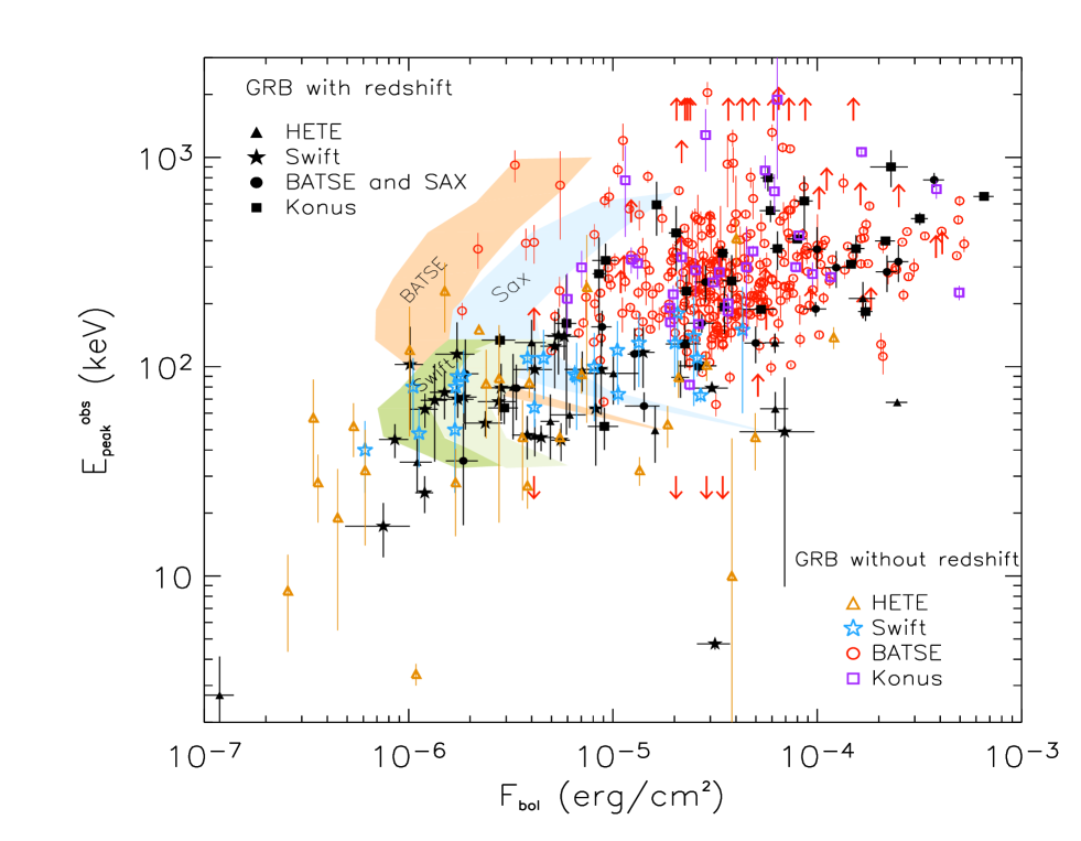
Figure 1: Distribution in the $E^{\rm obs}_{\rm peak}$–$F$ plane of the GRBs with measured redshift (filled symbols) and bursts without measured $z$ published in the literature (open symbols). The bolometric fluence is obtained by integrating the spectrum in the range 1 keV–10 MeV. The bright BATSE sample (from K06) is shown by open circles (for well constrained $E^{\rm obs}_{\rm peak}$) and up/down arrows (when only an upper/lower limit can be set on $E^{\rm obs}_{\rm peak}$ from the spectral analysis of K06). Hete–II (Sakamoto et al. 2005) and Swift bursts (B07 – but see text) without redshifts are shown with open triangles and stars, respectively. Shaded regions represent the ST curves of minimum fluence, for different instruments (see G08 for more details), down to which it is possible to fit the spectrum and constrain the spectral parameters.

2 The $E^{\rm obs}_{\rm peak}$–Fluence plane

The observer frame $E^{\rm obs}_{\rm peak}$–$F$ correlation, found using $z$GRBs (filled symbols in Fig. 1), divides the plane in two regions corresponding to large fluence and low/moderate $E^{\rm obs}_{\rm peak}$ (region–I) and low fluence and large/moderate $E^{\rm obs}_{\rm peak}$ (region–II). The absence of bursts in region–I suggests that they are extremely rare because, otherwise, they would have been easily detected by present and past GRB detectors. The absence of bursts in region–II could be due to selection effects.

In the following we will refer to GRBs with known $z$ as $z$GRBs and we will indicate bursts without measured $z$ as GRBs.

2.1 GRB samples with redshifts: $z$GRBs

Different detectors/satellites (BATSE–CGRO, Hete–II, Konus–Wind, BeppoSAX, Swift) have been contributing the sample of GRBs with measured $z$ and $E^{\rm obs}_{\rm peak}$, possibly introducing different instrumental selection effects. G08, by considering the trigger efficiency of these satellites (from Band 2003), excluded that this is affecting the sample of 76 bursts defining the $E^{\rm obs}_{\rm peak}$–$F$ correlation. However, a stronger selection effect was studied in G08: to add a point in the $E_{\rm peak}-E_{\rm iso}$ correlation, in addition to detect it, we need to determine (through the spectral analysis) the peak energy $E^{\rm obs}_{\rm peak}$. This requires a minimum fluence. G08 simulated several spectra of GRBs by assuming they are described by a Band function. The values assumed for the low and high energy indeces are fixed to the typical values $\alpha=-1$ and $\beta=-2.3$. By varying the peak energy, the fluence and the duration G08 derived the “spectral analysis thresholds” ST (shaded curves in Fig. 1) in the $E^{\rm obs}_{\rm peak}$–$F$ plane for BATSE, BeppoSAX and Swift. Details of the simulations are given in G08. These curves show that the limiting fluence $F$ is a strong function of $E^{\rm obs}_{\rm peak}$. A burst on the right side of these curves has enough fluence to constrain its peak spectral energy. As discussed in G08, Fig. 1 shows that the 27 Swift bursts (filled stars) with $z$ and well constrained $E^{\rm obs}_{\rm peak}$ (from C07) are affected by this selection effect (dark and light grey areas labeled Swift in Fig. 1). Note that this is a small sub–sample of the bursts detected by Swift. Indeed, in order to add a point to the $E_{\rm peak}-E_{\rm iso}$ correlation, in addition to $z$, also $E^{\rm obs}_{\rm peak}$ is needed. C07, through the analysis of the BAT–Swift spectra of bursts with known $z$, showed that, given the limited energy range of this instrument (15–150 keV), the peak energy could be determined only for a small fraction of bursts. Therefore, these 27 Swift bursts are all the GRBs (up to April 2008) for which both the $z$ is known and $E^{\rm obs}_{\rm peak}$ could be determined from the fit of the BAT–Swift spectrum. The fact that the Swift sample, for which the spectral analysis of C07 yielded $E^{\rm obs}_{\rm peak}$, extends to the estimated limiting ST is an independent confirmation of the reliability of the method for simulating these curves. Note that a few Swift bursts are below these lines, but in these cases the peak energy was found using the combined XRT–BAT spectrum (see G08).

Instead, pre–Swift $z$GRBs (partly detected by BATSE and BeppoSAX – filled circles in Fig. 1) are not affected by the corresponding ST curves. Note that only for BATSE we could derive the ST through our simulations. To this aim, the detector response and background model is needed. For Konus–Wind, BeppoSAX and Hete–II these informations are not public. However, for BeppoSAX we can rescale the BATSE thresholds (see G08 for details).

The sample of $z$GRBs considered in this work contains 83 objects, 76 from the sample collected in G08, plus 7 bursts recently detected (up to April 2008). For all these 7 bursts the spectral parameters come from fitting the Konus–Wind spectra and are reported in the GCN circulars (see Tab. 3). With this updated sample we find an Amati correlation with slope $s=0.48\pm 0.03$ and scatter $\sigma=0.23$. The same sample defines also a correlation (Kendall’s $\tau=0.51$) in the observer plane in the form $E^{\rm obs}_{\rm peak}\propto F^{0.40\pm 0.05}$.

A way to investigate if the lack of GRBs in region–II of the $E^{\rm obs}_{\rm peak}$–$F$ plane, i.e. between the distribution of bursts with $z$ and the ST curves defined in G08, is real or it is due to a still unexplained selection effect is to consider all GRBs with well constrained $E^{\rm obs}_{\rm peak}$ but without measured $z$.

2.2 GRB samples without $z$

We consider Hete–II bursts (Sakamoto et al. 2005), Swift bursts (from B07), the bright BATSE sample (K06) and Konus–Wind bursts (Golenetskii et al. 2005, 2006, 2007, 2008, GCN circulars). Through these samples we populate the $E^{\rm obs}_{\rm peak}$–$F$ plane.

2.2.1 Bright BATSE bursts

We have considered the sample of 350 BATSE GRBs published by K06. The selected bursts have either a peak photon flux (in the 50–300 keV energy range) larger than 10 [photon s^-1 cm^-2] or a fluence (integrated above 25 keV) larger than 2$\times 10^{-5}$ [erg cm^-2]. We excluded the 17 events whose spectrum was accumulated for less than 2 sec as most likely representative of the short duration burst population. With the remaining GRBs, we constructed a first sample selecting all bursts whose time integrated spectrum is fitted with a curved model (Band, cutoff power–law or smoothly–joined power law) providing an estimate of $E^{\rm obs}_{\rm peak}$. This sample contains 279 GRBs. The remaining bursts form another sample providing lower/upper limits on $E^{\rm obs}_{\rm peak}$: those GRBs fitted with a Band or smoothly–joined power law with an high energy photon index greater than –2 provide a lower limit, as well as those fitted with a single flat power law. On the contrary, bursts fitted by single steep power laws (photon index $<-2$) provide an upper limit on $E^{\rm obs}_{\rm peak}$.

Fig. 1 shows the K06 sample (open circles) in the $E^{\rm obs}_{\rm peak}$–$F$ plane together with the 83 $z$GRBs. The BATSE ST curves are also shown. By comparing BATSE GRBs with $z$GRBs (filled symbols in Fig. 1) we note that the two samples are consistent for $E^{\rm obs}_{\rm peak}$ values in the 100 keV – 1 MeV range. However, note that in the K06 sample there are also a few bursts with considerably smaller fluence (but similar $E^{\rm obs}_{\rm peak}$) with respect to $z$GRBs. In other words, there is an indication of the existence of bursts that lie between the limiting BATSE curves and the $E^{\rm obs}_{\rm peak}$–$F$ correlation defined by $z$GRBs (region–II). From Fig. 1 it is clear that the sample of bright BATSE bursts is not strongly affected by the corresponding ST. However, note that this sample is not appropriate to study this issue because it is representative only of very bright BATSE bursts and it is not complete in fluence.

The K06 sample shows a weak $E^{\rm obs}_{\rm peak}$–$F$ correlation with a Kendall’s correlation coefficient $\tau=0.13$ (3$\sigma$ significance).

2.2.2 Swift and Hete–II bursts

Other two samples of bursts with published spectral parameters are that of Hete–II and Swift. The two references for the Swift bursts are C07 and B07: the former focused on Swift bursts with $z$ and the latter considered also bursts without redshifts. The C07 Swift bursts were included in the sample of the 83 $z$GRBs. For the Swift bursts without $z$ we consider the analysis performed by B07 (but see also Sakamoto et al. 2008b). They analysed GRB spectra with either the frequentist method and through a Bayesian method. While the first method allows to constrain the spectral $E^{\rm obs}_{\rm peak}$ only if it lies in the energy range where the spectral data are (15–150 keV for BAT–Swift), the bayesian method infers the peak energy by assuming an $E^{\rm obs}_{\rm peak}$ distribution as prior. For homogeneity with the analysis of C07 and with the method used to find the ST, we consider only the Swift bursts of B07 without $z$ which have their peak energy estimated through the frequentist method and for which this estimate has a relative error $<$100%. This choice corresponds to the conditions of the simulated ST of G08. We found 22 Swift bursts which satisfy these requirements.

The Hete–II group published some spectral catalogs of their bursts (Barraud et al. 2003; Atteia et al. 2005; Sakamoto et al. 2005). Sakamoto et al. (2005) performed the time integrated spectral analysis of 45 GRBs detected during the first 3 years of the Hete–II mission. They performed spectral fits by combining the data of the high energy detector (Fregate: 6–400 keV) and the low energy coded mask detector (WXM: 2–25 keV). We have considered in this sample the 27 bursts without $z$ (the remaining are already included in the $z$GRB sample) and whose spectrum is fitted by a Band or cutoff power–law model which provides an estimate of $E^{\rm obs}_{\rm peak}$.

Fig. 1 shows that Swift bursts (open stars) and Hete–II bursts (open triangles) are both consistent with the correlation defined in the $E^{\rm obs}_{\rm peak}$–$F$ plane by the $z$GRB sample. Also the Swift sample without $z$ confirms the validity of the ST estimates. Note that the extension of Hete–II events at very low values of $E^{\rm obs}_{\rm peak}$ is due to the fit of their spectrum with the WXM instrument (see Sakamoto et al. 2005).

Note that in the sample of 83 bursts with $z$ there are also the BeppoSAX and Konus–Wind events. No spectral catalog of bursts without redshifts has been published to date for these two satellites.

2.2.3 Konus–Wind bursts

Preliminary results arising from the fit of Konus–Wind spectra can be found in the GCN circulars. We collected a sample of 29 GRBs (empty squares in Fig. 1) for which an estimate of $E^{\rm obs}_{\rm peak}$ and the spectral shape is available and which are not already included in the Hete–II or Swift samples considered above. For each burst we estimate the bolometric (1–10⁴ keV) fluence and the bolometric peak flux. The results are listed in Tab. 1 in the Appendix. Since Konus–Wind covers an energy range from 20 keV to a few MeV, a good spectral analysis of very hard bursts can be performed. Anyway, the determination of its TT and ST is not possible, as the background model and the detector response are not public. Therefore, with respect to the distribution of these GRBs in the $E^{\rm obs}_{\rm peak}$–$F$ plane (Fig 1), we can only note that it seems to be very similar to that of bright BATSE bursts (empty circles).

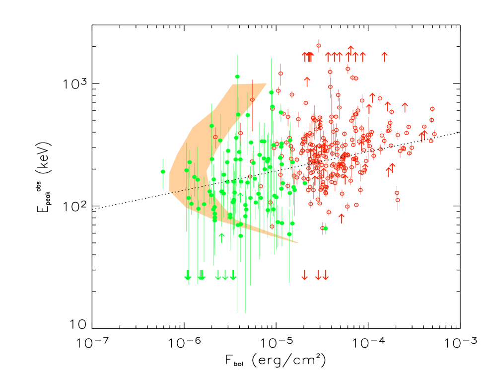
Figure 2: The $E^{\rm obs}_{\rm peak}$–$F$ plane for the sample of BATSE bursts. The fluence reported in this plot is the bolometric fluence (1–10⁴ keV). The open circles are GRBs of the K06 sample with catalog fluence larger than 2$\times 10^{-5}$ erg cm^-2 and the filled circles are the 100 GRBs analyzed in this paper. The arrows correspond to those bursts for which we can only estimate a lower/upper limit to $E^{\rm obs}_{\rm peak}$. The shaded region represents the minimum fluence requested to constrain $E^{\rm obs}_{\rm peak}$ from the spectral analysis. The left and right boundaries of this region are calculated for a burst lasting 5 and 20 seconds respectively (see G08 for more details). The dotted line represents the best fit to the combined sample: $E^{\rm obs}_{\rm peak}\propto F_{\rm bol}^{0.16\pm 0.02}$.

3 Faint BATSE bursts

Among the above sample, the bright BATSE bursts of K06 is the largest and, given the spectral range of BATSE, covers a wide range in $E^{\rm obs}_{\rm peak}$. However, this sample was selected according to a minimum peak flux or fluence threshold and it is not complete either in peak flux and fluence. Furthermore it extends down to a fluence larger than the the minimum fluence required to derive $E^{\rm obs}_{\rm peak}$.

Samples reaching smaller fluences indeed exist: Yonetoku et al. (2004) performed the spectral analysis of 745 GRBs from the BATSE catalog with flux larger than $2\times 10^{-7}$ [erg cm^-2 s^-1]. However, they exclude 56 GRBs for which they find a pseudo redshift greater then 12 or no solution using the $E_{\rm peak}-L_{\rm iso}$ relation as a distance indicator. Thus the final sample is biased by this choice as it most likely excludes the bursts with low fluence and intermediate/high peak energy and therefore is not representative of the whole sample of BATSE bursts with fluences greater than the spectral threshold.

It is clear from Fig. 1 that for BATSE bursts “there is room” to extend the K06 sample to smaller fluences: if the ST for BATSE are correct, we should be able to analyze bursts with fluence smaller than 2$\times 10^{-5}$ [erg cm^-2]. Therefore, in order to increase the statistics and test the density of bursts in region–II we extend the BATSE sample to the limiting fluence of 10^-6 [erg cm^-2]. To this aim we selected a representative sample of 100 BATSE bursts with a fluence $F$ above 25 keV (which is a good proxy for the bolometric fluence), within the range $10^{-6}<F<2\times 10^{-5}$ [erg cm^-2]. The number of extracted GRBs per fluence bin follows the Log$N$–Log$F$ distribution and therefore this sub–sample is representative of the BATSE burst population in this fluence range (which corresponds to $\sim 1000$ events).

For all these bursts we analysed the BATSE Large Area Detector (LAD) spectral data which consist of several spectra accumulated in consecutive time bins before, during and after the burst. The spectral analysis has been performed with the software SOAR v3.0 (Spectroscopic Oriented Analysis Routines), which we implemented for our purposes. For each burst we analysed the BATSE spectrum accumulated over its total duration (which in most cases corresponds to the $T_{90}$ parameter reported in the BATSE catalog). In order to account for the possible time variability of the background we modeled it as a function of time (see e.g. K06).

In most cases we could fit either the Band model (Band et al. 1993) or a cutoff power law model. To be consistent with the method used to derive the spectral threshold curves of Fig. 1, we consider that $E^{\rm obs}_{\rm peak}$ is reliably determined if its relative error is less than 100%. If the relative error is greater or if the best fit model is a simple power law we derive the corresponding lower/upper limit. In these cases the burst is reported on the plot as an up/down arrow.

In Tab. 2 in the appendix we list the bursts of our sample together with the results of the spectral fitting.

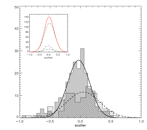
Figure 3: Scatter distributions of the sample of BATSE bursts with well estimated $E^{\rm obs}_{\rm peak}$ around their best fit correlation in the $E^{\rm obs}_{\rm peak}$–$F$ plane (see Fig.  2). The shaded distribution is of the 213 GRBs of K06 and the hatched distributions is of the 88 GRBs of our analysis (we have excluded upper/lower limits). The fit with gaussian functions of the two distributions have scatter $\sigma=0.18$ for the K06 sample and $\sigma=0.29$ for our sample. The insert shows the scatter of the combined sample ($\sigma=0.26$) (solid line), once we take into account that the GRBs analyzed by us are representative of 1000 bursts.

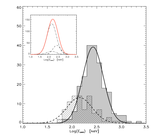
Figure 4: The $E^{\rm obs}_{\rm peak}$ distributions for the K06 GRB sample (213 GRBs – shaded histogram) and for the sample that we have analyzed (88 GRBs with well determined $E^{\rm obs}_{\rm peak}$ over 100 bursts randomly extracted from the BATSE Log$N$–Log$F$ distribution in the range $10^{-6}<F<2\times 10^{-5}$ [erg cm^-2] – hatched histogram). The solid and dashed lines are the gaussian fits to the two distributions. The K–S test (see text) confirms that the shift of $E^{\rm obs}_{\rm peak}$ to lower values for dimmer bursts is statistically significant. In the insert are reported these two gaussian fits and their sum (solid line) which has been obtained by multiplying the distribution of the 100 GRBs by 10 (dot–dashed line) in order to account for the total number of bursts in this fluence range.

3.1 Results for the complete sample of BATSE bursts

In order to construct a complete sample of BATSE bursts, we cut the K06 sample at a fluence $F$ (as reported in the BATSE catalog) greater than $2\times 10^{-5}$ [erg cm^-2] (213 GRBs). This complete sub–sample is representative of bright BATSE bursts. To this we add the 100 bursts of our representative sample of the 1000 GRBs with fluences between $10^{-6}$ and 2$\times 10^{-5}$ [erg cm^-2]. Fig. 2 shows the $E^{\rm obs}_{\rm peak}$ and bolometric fluence (computed in the range 1 keV – 10 MeV) of the sub–sample of bursts from the K06 sample (open circles) together with the 100 bursts of our sample (filled circles). This combined sample extends the K06 fluence limit to $F>10^{-6}$ erg cm^-2. Note that in this figure we plot the bolometric (1-10⁴ keV) fluence estimated accordingly with the best fit model. Its value can be different from the fluence value reported in the BATSE catalog.

The distribution of BATSE GRBs in Fig. 2 defines a correlation with a large scatter. The Kendall’s correlation coefficient is $\tau=0.18$ (7$\sigma$ significant). Since the dimmer part of the burst distribution in the $E^{\rm obs}_{\rm peak}$–$F$ plane is affected by the ST truncation effect, we analyzed the correlation also following the method proposed by Lloyd et al. (2000). We obtain a Kendall’s correlation coefficient $\tau=0.2$ (5.5$\sigma$ significant). By fitting with the least square method, without weighting for the errors and neglecting the upper/lower limits, we obtain $E^{\rm obs}_{\rm peak}\propto F_{\rm bol}^{0.16\pm 0.02}$ (dotted line in Fig. 2).

In Fig. 3 we show the distribution of the scatter of the two samples around the best fit correlation in the $E^{\rm obs}_{\rm peak}$–$F$ plane. These have standard deviation of $\sigma$=0.18 for the K06 sample (solid histogram) and $\sigma~{}$=0.29 for our representative sample (hatched histogram). The combined sample (solid line in the insert) has a scatter distribution with $\sigma~{}$=0.26. In order to describe the scatter distribution of BATSE bursts down to the fluence limit of $F>10^{-6}$ [erg cm^-2], we have to consider that our sample of 100 bursts is representative of the entire burst population (a factor 10 larger in number) in the fluence range $10^{-6}<F<2\times 10^{-5}$ [erg cm^-2]. We fitted the scatter distributions of our (dashed line) and K06 (solid line) sample with gaussian functions and combined these best fit distributions by renormalizing that of our sample by a factor 10 (corresponding to the ratio of the extracted bursts with respect to the total number of BATSE bursts in the same fluence bin). The result is shown in the insert of Fig. 3 (solid line). The combined sample (solid line in the insert) has a scatter distribution with $\sigma$=0.26.

Fig. 2 shows that there are bursts with low fluence and high $E^{\rm obs}_{\rm peak}$ and that the dispersion in $E^{\rm obs}_{\rm peak}$ at low fluence is larger then the dispersion at high fluence. However, Fig. 2 also shows that, on average, the error on the $E^{\rm obs}_{\rm peak}$ value increases for smaller fluences. This could imply that the larger scatter for smaller fluences is in part due to larger errors on $E^{\rm obs}_{\rm peak}$. A simple way to determine the contributions to the total observed scatter $\sigma_{\rm tot}$, calculated orthogonally to the fitting line, is:

$$\sigma_{\rm tot}^{2}\,=\,\sigma^{2}_{E}\cos^{2}\theta+\sigma^{2}_{\rm c}$$ (1)

where $\sigma^{2}_{E}$ is the average relative error on $E^{\rm obs}_{\rm peak}$, $\theta$ is the angle defined by the slope of the correlation (whose angular coefficient is equal to $\tan\theta=0.16$) and $\sigma_{\rm c}$ is the intrinsic scatter of the distribution. For fluences greater than 2$\times 10^{-5}$ [erg cm^-2] (K06 sample) $\sigma_{\rm tot}\sim\sigma_{\rm c}=0.18$ since the errors on $E^{\rm obs}_{\rm peak}$ are small. On the other hand, for fluences smaller than 2$\times 10^{-5}$ [erg cm^-2] (our sample), $\sigma_{E}=0.18$ and $\sigma_{\rm tot}=0.29$, leading to $\sigma_{\rm c}=0.23$, to be compared to $\sigma_{\rm c}=0.18$ for fluences greater than 2$\times 10^{-5}$ [erg cm^-2]. This leads us to conclude that the intrinsic scatter around the best fit line increases for smaller fluences. A caveat is in order: the scatter $\sigma_{\rm c}$ does not take into account lower/upper limits, which also do not enter in the derivation of the best fit line. Thus $\sigma_{\rm c}$ could be larger, but only slightly, since the number of upper/lower limits is very limited.

Through our BATSE sample we can also study the $E^{\rm obs}_{\rm peak}$ distribution. In Fig. 4 we show the $E^{\rm obs}_{\rm peak}$ distribution of our BATSE sample (hatched histogram) and that of bright BATSE bursts of K06 (solid filled histogram – cut at 2$\times 10^{-5}$ [erg cm^-2]).

The shift of the $E^{\rm obs}_{\rm peak}$ distribution to lower values for smaller fluence selection is statistically significant: the K–S test gives a probability $P=5.8\times 10^{-11}$ that the two distributions belong to the same population. Similarly to what has been done for the scatter distribution, we combine the two distributions by accounting for the fact that our sample is representative of a larger population of bursts in the $10^{-6}$– 2$\times 10^{-5}$ [erg cm^-2] fluence range. The result is shown in the insert of Fig. 4 (solid line). This total sample distribution has a peak at $E^{\rm obs}_{\rm peak}$$\sim$160 keV, i.e. smaller than the 260 keV of bright bursts of K06, and a standard deviation $\sigma$=0.28. Although the widths of the distributions of $E^{\rm obs}_{\rm peak}$ can be affected by the measurement errors, the central values are not.

4 Outliers of the $E_{\rm peak}-E_{\rm iso}$ correlation

In Fig. 5 we combine, in the $E^{\rm obs}_{\rm peak}$–$F$ plane, our sample of BATSE bursts with the $z$GRBs (solid filled squares) and with the Swift, Hete–II and Konus–Wind samples of GRBs without redshifts.

We note that bursts with known redshift (filled squares) are only representative of the large fluence (for any $E^{\rm obs}_{\rm peak}$) part of the plane. In particular, Fig. 5 shows the existence of bursts with low fluence (between $F\leq 10^{-6}$ and $F\sim 10^{-5}$ [erg cm^-2]) but $E^{\rm obs}_{\rm peak}$ larger than 200 keV. These events are not present in the $z$GRB sample. Their absence in the $z$GRB sample suggests the existence of a selection effect.

However, $z$GRBs are those defining the Amati correlation (as in G08). We do not know if all the other bursts (without redshifts) represented in Fig. 5 satisfy this correlation.

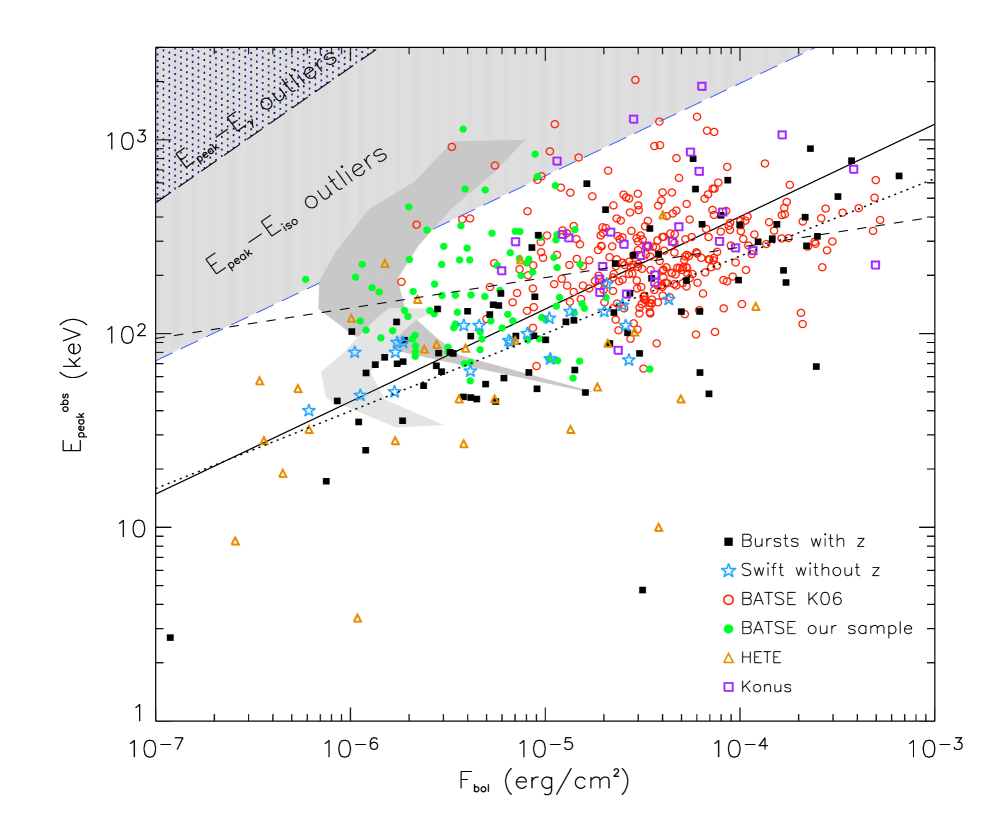
Figure 5: Consistency test of the $E_{\rm peak}-E_{\rm iso}$ correlation. The open symbols represent the bursts without redshifts detected by Hete–II (triangles), BATSE (open and filled circles), Swift (open stars) as described in the legend. The solid line is the $E_{\rm peak}-E_{\rm iso}$ correlation transformed in the observer $E^{\rm obs}_{\rm peak}$–$F$ plane. The long–dashed line is the 3$\sigma$ scatter of the $E_{\rm peak}-E_{\rm iso}$ correlation. The “region of outliers” is the grey shaded. Bursts falling in this region are not consistent with the $E_{\rm peak}-E_{\rm iso}$ correlation for any redshift: they are outliers at more than $3\sigma$ (if the scatter distribution is Gaussian, see text). In the upper left corned we also show the “region of outliers” of the $E_{\rm peak}-E_{\gamma}$ correlation (adapted from Ghirlanda et al. 2007) if bursts have a 90^∘ jet opening angle. The dotted line is the fit to the $z$GRB sample (filled squares) and the dashed line is the fit to the complete sample of BATSE bursts described in Sec.3.1 (see also Tab.1)

If these GRBs have a similar redshift distribution of those with measured $z$, then it is likely that they would define a rest frame $E_{\rm peak}-E_{\rm iso}$ correlation with different properties (slope, normalization and scatter), since some of them stay apart from the $E^{\rm obs}_{\rm peak}$–$F$ correlation defined by the $z$GRB sample. On the other hand, GRB 980425 and GRB 031203 do have a peak energy and fluence consistent with the $z$GRB sample, but it is their small redshift to make them outliers with respect to the $E_{\rm peak}-E_{\rm iso}$ correlation.

The possibility that there is a considerable number of outliers of the $E_{\rm peak}-E_{\rm iso}$ correlation in the BATSE sample has been discussed in the literature (e.g. Nakar & Piran 2005; Band & Preece 2005; K06 – but see also Ghirlanda et al. 2005; Bosnjak et al. 2007). We can test if a burst is consistent or not with the $E_{\rm peak}-E_{\rm iso}$ correlation even if we do not know its redshift. Simply, we assign to the burst any redshift, checking if there is at least one $z$ making it consistent with the correlation. By “consistent” we mean the the burst must fall within the 3$\sigma$ scatter (assumed gaussian) of the correlation. This test was first proposed for the short bursts (Ghirlanda et al. 2004a) and then applied to BATSE long GRBs. More quantitatively, following Nakar & Piran (2005), we can write the $E_{\rm peak}-E_{\rm iso}$ correlation as

$$E_{\rm peak}^{\rm obs}(1+z) = k\left({4\pi d_{\rm L}^{2}F\over 1+z}\right)^{a}\,\,\to$$

$$E_{\rm peak}^{\rm obs} = kF^{a}f(z);\qquad f(z)={(4\pi d_{\rm L}^{2})^{a}\over(1+z)^{1+a}}$$ (2)

where $F$ is the bolometric fluence. The function $f(z)$ has a maximum ($f_{\rm max}$) at some redshift and therefore all bursts for which $E_{\rm peak}^{\rm obs}/(kF^{a})>f_{\rm max}$ are outliers. We can impose that the constant $k$ accounts for the scatter of the best fit $E_{\rm peak}-E_{\rm iso}$ correlation, and then find outliers at some pre–assigned number of $\sigma$. It is worth to recall that this method assumes that the dispersion of points, around the $E_{\rm peak}-E_{\rm iso}$ correlation under test, is described by a Gaussian function. With this assumption we can state that a given GRB is $N\sigma$ inconsistent with the correlation, and quantify the probability of having a certain number of outliers lying – say – more than 3$\sigma$ away. Since the Amati correlation, as discussed below, surely incorporates an extra–Poissonian dispersion term (Amati, 2006), the scatter distribution may not be a Gaussian, but it may correspond to the distribution function of this extra term. In other words: the scatter of the points around the Amati correlation is not due to the errors of our measurements, but reveals the presence of an extra–observable not considered in the Amati relation. With this caveat, we nevertheless use this assumption (i.e. Gaussianity) for simplicity.

In Fig. 5 the grey area identifies, in the $E^{\rm obs}_{\rm peak}$–$F$ plane, the “region of outliers”. Considering only BATSE bursts we can state that the 6% of the complete sample considered in this paper is constituted by bursts which are surely outliers of the $E_{\rm peak}-E_{\rm iso}$ relation. We can test if these outliers have different spectral properties with respect to other bursts (that instead pass the above consistency test). By comparing their spectral parameters we find that the outliers of the $E_{\rm peak}-E_{\rm iso}$ correlation have a larger peak energy than the total sample of bursts (K–S probability $P=8.7\times 10^{-5}$) and a slightly harder low energy spectral index $\alpha$ (K–S probability $P=10^{-1}$). From Fig. 5 we also note that there is no outlier for the $E_{\rm peak}$-$E_{\gamma}$ correlation.

correlation	sample	scatter	K	s
$E_{\rm peak}-L_{\rm iso}$	$z$GRB	0.28	–18.6	0.40$\pm$0.03
	$z$GRB (only Swift)		–11.4	0.26$\pm$0.05
	$z$GRB (not Swift)		–20.5	0.44$\pm$0.03
$E_{\rm peak}-E_{\rm iso}$	$z$GRB	0.23	–22.7	0.48$\pm$0.03
	$z$GRB (only Swift)		–16.7	0.36$\pm$0.06
	$z$GRB (not Swift)		–24.4	0.51$\pm$0.03
$E^{\rm obs}_{\rm peak}$–$P$	$z$GRB	0.26	4.41	0.39$\pm$0.05
	BATSE	0.20	3.93	0.28$\pm$0.02
$E^{\rm obs}_{\rm peak}$–$F$	$z$GRB	0.23	4.00	0.40$\pm$0.05
	BATSE	0.23a	3.07	0.16$\pm$0.02

Table 1: Results of the correlation analysis. For each correlation in the rest frame and observed plane we give the values of the scatter, normalization and slope. The correlations are in the form $y=Kx^{s}$, where y is the logarithmic observed/rest frame peak energy in units of keV and x is the logarithm of the luminosity (energy) in erg s^-1 (erg) or the peak flux (fluence) in erg cm^-2 s^-1 (erg cm^-2). $a$: this is the value once depurated of the contribution to the scatter of the measurement errors (see text).

5 The $E_{\rm peak}-L_{\rm iso}$ correlation

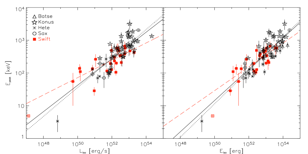
Figure 6: $E_{\rm peak}-L_{\rm iso}$ and $E_{\rm peak}-E_{\rm iso}$ correlations for 83 GRBs with measured redshift and spectral parameters. The best fit of the whole sample is shown with a solid line. Note that the fit performed on the Swift sample alone (filled squares) has in both cases a very flat slope (dashed line) with respect to the slope derived for no–Swift bursts (dotted line). The results of these different analysis are reported in Tab. 1. For an explaination of the flat slope found with the Swift sample see G08.

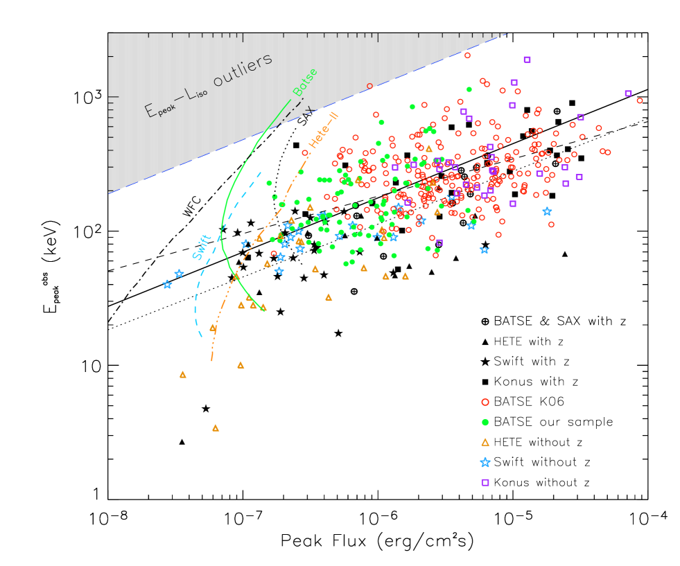
Figure 7: Consistency test of the $E_{\rm peak}-L_{\rm iso}$ correlation. The filled squares are bursts with measured redshifts. The solid line is the $E_{\rm peak}-L_{\rm iso}$ correlation transformed in the observer $E^{\rm obs}_{\rm peak}$–$P$ plane (here it is represented the bolometric peak flux). The long dashed line is the 3$\sigma$ scatter of the $E_{\rm peak}-L_{\rm iso}$ correlation (as discussed in Sec. 5). The shaded triangle delimits the “region of outliers”. Bursts falling in this region are not consistent with the $E_{\rm peak}-L_{\rm iso}$ correlation for any redshift: they are outliers at more than $3\sigma$ (if the scatter distribution is Gaussian, see text). The dotted and dashed lines show the best fit obtained by considering respectively the $z$GRB sample and the BATSE complete sample. The curves represent the TT estimated for different instruments by assuming that the trigger is based on the peak flux criterion.

Yonetoku et al. (2004, Y04), with a sample of 16 GRBs of known $z$, found that $E_{\rm peak}$$\propto L_{\rm iso}^{0.5}$, where $L_{\rm iso}$ is the isotropic luminosity at the peak of the prompt light curve, but calculated using the time averaged spectrum (i.e. $E_{\rm peak}$ and spectral indices), and not the spectral properties at the peak flux.

This correlation appeared to be tighter (but with similar slope) than the $E_{\rm peak}-E_{\rm iso}$ correlation, as originally found by Amati et al. (2002). Since then this correlation has been updated only once (Ghirlanda et al., 2005b).

It is interesting to test if the same conclusions that can be drawn for the $E_{\rm peak}-E_{\rm iso}$ correlation (i.e. the presence of selection effects and of outliers) can now be extended to the $E_{\rm peak}-L_{\rm iso}$ correlation. To this aim we have considered the $z$GRB sample (see Tab. 3 in the Appendix) and we have calculated for all these bursts their isotropic equivalent luminosity $L_{\rm iso}$. This is computed by integrating the time averaged spectrum after renormalizing it with the peak flux. Note that, strictly speaking, this luminosity does not correspond to the peak luminosity (see Ghirlanda et al. 2005b), since it adopts the time averaged $E^{\rm obs}_{\rm peak}$.

In Tab. 3 we report the sample of 83 GRBs with their peak flux, the energy range where it is computed, the references and $L_{\rm iso}$. To calculate $L_{\rm iso}$ we adopted the same method used to compute $E_{\rm iso}$ (see Ghirlanda et al. 2007 for more details).

In Fig. 6 we show the $E_{\rm peak}-L_{\rm iso}$ and the $E_{\rm peak}-E_{\rm iso}$ correlations defined with the 83 GRBs of Tab. 3. The no–Swift bursts (empty symbols) and the Swift bursts (filled squares) are shown. In both cases, the correlations are highly significant (rank correlation coefficient are respectively 0.83 with a chance probability $6.2\times 10^{-22}$ and 0.84 with a chance probability $9.8\times 10^{-23}$). The solid lines show the best fit with the least square method (without accounting for the measurement errors): we obtain $E_{\rm peak}$$\propto L_{\rm iso}^{0.40\pm 0.03}$ and $E_{\rm peak}$$\propto E^{0.48\pm 0.03}_{\rm iso}$. The fits of the no–Swift burst sample (dotted line) and of the Swift burst sample (dashed line) are also shown. The results of these fits performed considering different samples are shown in Tab. 1.

Our sample of 83 $z$GRBs confirms the finding of Yonetoku et al. (2004), even if we obtain a flatter slope. Fitting the scatter distribution of the $E_{\rm peak}-L_{\rm iso}$ correlation with a Gaussian we derive $\sigma=0.28$. Comparing it with the corresponding scatter of the $E_{\rm peak}-E_{\rm iso}$ correlation ($\sigma=0.23$) we find that, contrary to what initially found by Yonetoku et al. (2004), the scatter of this correlation is slightly larger.

We can investigate if this correlation is affected by any of the selections effects that have been studied in G08 for the $E_{\rm peak}-E_{\rm iso}$ correlation. In particular we show in Fig. 7 the observer frame $E^{\rm obs}_{\rm peak}$–$P$ correlation where $P$ is the bolometric peak flux. Note that also in this plane the $z$GRBs define a strong correlation (dotted line – with slope 0.39) and that the GRB samples without $z$ considered in this work are consistent with this correlation (differently to what happens in the $E^{\rm obs}_{\rm peak}$–$F$ plane). The dashed line represents the best fit obtained considering only BATSE bursts. They define a flatter correlation (slope 0.28) with respect to the $z$GRB sample. Note that this happens also in the $E^{\rm obs}_{\rm peak}$–$F$ correlation and it is likely due to the difficulty of the BATSE instrument to see very low $E^{\rm obs}_{\rm peak}$ at low fluence/peak flux.

The peak flux $P$ is the quantity on which the trigger condition (for most instruments) is determined. We plot in Fig. 7 the trigger limiting curves (from G08) as a function of $E^{\rm obs}_{\rm peak}$. We note that for BATSE the TT curve is separated from the distribution of the corresponding bursts (open and filled circles). This is because the dominant selection effect acting on our BATSE complete sample is the ST (see Fig. 2). In other words, the bursts that can be displayed in the $E^{\rm obs}_{\rm peak}$–$P$ plane are not all the bursts that can be detected by a given instrument, but only those with a sufficient number of photons to make possible the determination of $E^{\rm obs}_{\rm peak}$.

The Hete–II bursts, instead (triangles), are very near to their TT. For this instrument we are not able to determine the ST curves, but it is likely that the dominant selection effect acting on Hete–II bursts is the need to trigger them.

For Swift bursts we have an intermediate case: their TT curve is not truncating their distribution, even if they lie closer (than BATSE bursts) to it.

Also for the $E_{\rm peak}-L_{\rm iso}$ correlation we can test if there are outliers. Ghirlanda et al. (2005b) tested this through a sample of 442 GRBs with redshifts derived by the lag–luminosity relation. They did not find evidence for outliers. In this work we test the $E_{\rm peak}-L_{\rm iso}$ correlation with the same method described above for the $E_{\rm peak}-E_{\rm iso}$ correlation. In Fig. 7 we show the “region of outliers” for the $E_{\rm peak}-L_{\rm iso}$ correlation. Only one burst (of the K06 sample) is inconsistent with this correlation at more than 3$\sigma$.

6 Discussion and conclusions

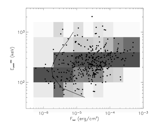
Figure 8: Graphic illustration of the $E^{\rm obs}_{\rm peak}$–$F$ correlation. We consider different fluence–bins and in each of those we count the total number $N_{f}$ of objects. Then we divide this fluence–bin into $E^{\rm obs}_{\rm peak}$–bins, counting the number of objects in each small area, dividing it by $N_{f}$. Each small area is then characterized by a number $n_{i,f}$ (between 0 and 1), which corresponds to a different level of grey. In this way the increasing number of bursts for decreasing fluence (the “Log$N$–Log$S$” effect) is accounted for, and it does not influence $n_{i,f}$. Note that the data points do not fill the entire accessible region of the plane (to the right of the ST curve shown in Fig. 2), but concentrate along a stripe.

To study the role of possible instrumental selection effects on the Amati relation we have focused our attention on the observational $E^{\rm obs}_{\rm peak}$–$F$ plane. Here we can compare the distribution of different samples of GRB (for example, $z$GRBs and GRB with unknown redshift). To this aim we adopt the analysis performed by G08, referring to two different instrumental biases: the trigger threshold (TT, the minimum fluence derived considering the minimum flux required to trigger a burst) and the spectral analysis threshold (ST, the minimum fluence needed to constrain the GRB spectral properties). These curves depends on $E^{\rm obs}_{\rm peak}$ and define what part of the observational plane is accessible.

First we updated the sample of bursts with redshift, adding 7 new recent GRBs, for a total of 83 objects. These GRBs define a $E_{\rm peak}$$\propto$$E_{\rm iso}$^0.48±0.03 correlation in the rest frame, very similar to that obtained with previous (and smaller) samples. In the observer plane, they define a slightly flatter correlation ($E^{\rm obs}_{\rm peak}$$\propto F^{0.40\pm 0.05}$). The scatter of these two correlations is the same (see Tab. 1). As G08 pointed out, the BATSE ST curve is not biasing the distribution of BATSE bursts with redshift in the observer plane, while the Swift ST could, in the sense that the distribution of Swift bursts (with redshift) is truncated by the Swift ST curve. Then why the BATSE bursts (with redshift) are not truncated by their corresponding ST? Is it because of a real, intrinsic correlation or is it due to another, hidden, selection effect? One way to answer this crucial question is to analyze all GRBs with $E^{\rm obs}_{\rm peak}$, even without redshift. The BATSE sample of GRBs is the best suited for this aim because: i) it contains a large number of bursts; ii) large sample of bright GRBs have been already analyzed, and iii) for BATSE we already know the ST curve. Then we pushed the spectral analysis to the limit, deriving the spectral parameters for a representative sample of 100 BATSE GRBs with a (bolometric) fluence between $10^{-6}$ [erg cm^-2] (corresponding to the ST limit) and $2\times 10^{-5}$ [erg cm^-2] (the limiting fluence of K06). These 100 GRBs represent a large population of 1000 GRBs, in the same fluence range. Combining our and the K06 samples we have a homogeneous and complete sample, best suited to study how BATSE GRBs populate the $E^{\rm obs}_{\rm peak}$–$F$ plane. Using this complete, fluence limited, sample we find:

• GRBs without redshifts, in this plane, are not spread in the region free from instrumental selection effects, but define a correlation with a flat slope ($\sim 0.16$) and a scatter larger for smaller fluences (after accounting for the errors increasing for smaller fluences). Fig. 8 is a graphic illustration of this: different grey levels corresponds to different density of points in the $E^{\rm obs}_{\rm peak}$–$F$ plane, once we take out the effect of the overall increase in density going to smaller fluences (for the Log$N$–Log$S$ slope). The way we do this is the following: we consider different fluence–bins and in each of those we count the total number $N_{f}$ of objects. Then we divide this fluence–bin into $E^{\rm obs}_{\rm peak}$–bins, counting the number of objects in each small area, dividing it by $N_{f}$. Each small area is then characterized by a number $n_{i,f}$ (between 0 and 1), which corresponds to a different level of grey. Note that the data points do not fill the entire accessible region of the plane but concentrate along a stripe. Note that the shape of this concentration of points is not determined by the ST curve, reported in Fig. 8 for a typical burst lasting 20 s. The only effect of the ST curve to the found correlation is to cut it at the smallest fluences and $E^{\rm obs}_{\rm peak}$. The very flat slope could be due to the difficulty of having BATSE GRBs with $E^{\rm obs}_{\rm peak}$ smaller than $\sim 50$ keV, whose existence is demonstrated by other instruments. However, the paucity of the derived upper limits on $E^{\rm obs}_{\rm peak}$ suggests that this effect is marginal.

• Formally, the scatter is not greater than the scatter of the $E_{\rm peak}-E_{\rm iso}$ correlation (both have $\sigma=0.23$ once the contribution to the scatter of the measurement errors are taken into account). Despite that, the entire BATSE sample and the $z$GRB population define two $E^{\rm obs}_{\rm peak}$–$F$ correlations which have significantly different slopes. If their redshift distribution is similar, then they will define two different correlations also in the $E_{\rm peak}-E_{\rm iso}$ plane: considering then the two samples together, we will define a correlation with intermediate slope and a scatter larger than the individual one.

• If the above point holds (i.e. if the redshift distributions of GRBs of unknown redshifts is the same of the $z$GRBs) then we can conclude that there exists an $E_{\rm peak}-E_{\rm iso}$  correlation, not determined by selection effects, even if its slope and scatter may be different from what we know now. We should emphasize that by the term ”correlation” we mean that GRBs will occupy a “stripe” in the $E_{\rm peak}-E_{\rm iso}$ plane with a relatively large scatter (fitting it with $\chi^{2}$ method one would obtain a very large reduced $\chi^{2}_{r}$). In other words, it is very likely that there is another (third) variable responsible for the scatter. In fact one finds a tighter correlation considering, as a third variable, the jet break time (Ghirlanda, Ghisellini & Lazzati 2004; Laing & Zhang 2005) or the time of enhanced prompt emission (Firmani et al. 2005). Another cause for a large scatter is the viewing angle, if a significant number of bursts are seen slightly off–axis.

• In the BATSE sample there are a few bursts with small or intermediate fluences but large $E^{\rm obs}_{\rm peak}$, not present in the $z$GRB sample. Among them there are some surely outliers of the $E_{\rm peak}-E_{\rm iso}$ correlation (as defined by the $z$GRB sample), i.e. bursts that lie at more than 3$\sigma$ from it, for any redshift. The number of these sure outliers is however very small, amounting to the 6 per cent of the entire population.

• We have also investigated the $E_{\rm peak}-L_{\rm iso}$ correlation, and its counterpart ($E^{\rm obs}_{\rm peak}$–$P$) in the observer plane. First, we partly confirm the original findings of Yonetoku et al. (2005, see also the update in Ghirlanda et al. 2005b): with the $z$GRB sample we find a strong $E_{\rm peak}-L_{\rm iso}$ correlation, whose slope is flatter than originally found ($s=0.40$ instead of 0.5) and whose scatter is greater than the scatter of the $E_{\rm peak}-E_{\rm iso}$ correlation.

• In the observer plane, instead, the $E^{\rm obs}_{\rm peak}$–$P$ correlation of our complete sample of BATSE bursts is tighter than the the $E^{\rm obs}_{\rm peak}$–$F$ correlation ($\sigma=0.2$ instead of $\sigma=0.23$). Its slope is $s=0.24$, flatter than the $E_{\rm peak}-L_{\rm iso}$ correlation ($s=0.39$), but however steeper than the $E^{\rm obs}_{\rm peak}$–$F$ slope ($s=0.15$). There is only one sure outlier.

• Selection effects are in this case determined by the TT curves. These effects are present, being responsible for the cutting at low peak fluxes, but they do not influence the slope and scatter for peak fluxes larger than the what defined by the TT curves.

• Considering the $z$GRB sample we have that the $E_{\rm peak}-E_{\rm iso}$ correlation is tighter than the $E_{\rm peak}-L_{\rm iso}$ one. Considering our complete BATSE sample and moving to the observer plane, we have just the opposite: the $E^{\rm obs}_{\rm peak}$–$P$ correlation is tighter than the $E^{\rm obs}_{\rm peak}$–$F$ one.

• It is then conceivable that the $E_{\rm peak}-L_{\rm iso}$ correlation, once a large number of burst with redshift will be available, will be stronger than the $E_{\rm peak}-E_{\rm iso}$ one.

The general conclusion we can draw from our study is that, although selection effects are present, they do not determine the spectral–energy and spectral–luminosity correlations. These could be characterized by a slope and scatter different from what we have determined now using heterogeneous bursts samples with measured redshift, but we found that $E_{\rm peak}$ is indeed correlated with the burst energetics or peak luminosity. Therefore it is worth to investigate the physical reason for this relation.

Appendix A Tables

GRB	$\alpha$	$\beta$	$E^{\rm obs}_{\rm peak}$	F	P	T	GCN
			keV	erg/cm2	erg/s/cm2	s
050326	-0.74$\pm 0.09$	-2.49$\pm 0.16$	201$\pm 24$	3.6e-5	6.8e-6	38	3152
050713A	-1.12$\pm 0.08$		312$\pm 50$	1.3e-5	1.8e-6	16	3619
050717	-1.12${}^{+0.17}_{-0.13}$		1890${}^{+1600}_{-760}$	6.3e-5	1.2e-5	50	3640
051008	-0.98${}^{+0.09}_{-0.08}$		865${}^{+178}_{-136}$	5.5e-5	9.8e-6	280	4078
051028	-0.73${}^{+0.26}_{-0.22}$		298${}^{+73}_{-50}$	7.0e-6	1.3e-6	12	4183
060105	-0.83$\pm 0.04$		424${}^{+25}_{-22}$	8.1e-5	6.7e-6	60	4439
060213	-0.83${}^{+0.05}_{-0.04}$		1061${}^{+83}_{-43}$	1.6e-4	7.1e-5	60	4763
060510A	-1.66${}^{+0.08}_{-0.07}$		184${}^{+36}_{-24}$	3.6e-5	6.1e-6	25	5113
060901	-0.77${}^{+0.26}_{-0.23}$	-2.31${}^{+0.18}_{-0.36}$	191${}^{+40}_{-30}$	1.9e-5	3.8e-6	8	5498
060904A	-1.00${}^{+0.23}_{-0.17}$	-2.57${}^{+0.37}_{-1.00}$	163$\pm 31$	1.9e-5	1.6e-6	80	5518
060928	-1.28$\pm 0.02$	-2.27${}^{+0.14}_{-0.21}$	705${}^{+74}_{-68}$	3.8e-4	3.1e-5		5689
061021	-1.22${}^{+0.14}_{-0.12}$		777${}^{+549}_{-237}$	1.1e-5	4.3e-6		5748
061122	-1.03${}^{+0.07}_{-0.06}$		160${}^{+8}_{-7}$	2.6e-5	9.9e-6	10	5841
061222A	-0.94${}^{+0.14}_{-0.13}$	-2.41${}^{+0.28}_{-1.21}$	283${}^{+59}_{-42}$	3.3e-5	7.0e-6	100	5984
070220	-1.21${}^{+0.29}_{-0.19}$	-2.02${}^{+0.27}_{-0.44}$	299${}^{+204}_{-130}$	4.4e-5	3.7e-6	130	6124
070328	-1.09$\pm 0.08$		688${}^{+173}_{-119}$	6.1e-5	4.7e-6	45	6230
070402	-0.92${}^{+0.12}_{-0.11}$		325${}^{+52}_{-40}$	1.2e-5	3.3e-6	12	6243
070521	-0.93$\pm 0.12$		222${}^{+27}_{-21}$	1.9e-5	4.4e-6	55	6459
070626	-1.45${}^{+0.04}_{-0.03}$	-2.28${}^{+0.08}_{-0.12}$	226${}^{+19}_{-17}$	4.9e-4	2.4e-5		6599
070724B	-1.15$\pm 0.13$		82$\pm 5$	2.3e-5	2.8e-6	50	6671
070821	-1.30$\pm 0.04$		268${}^{+19}_{-17}$	1.2e-4	1.5e-5	215	6766
070824	-1.05$\pm 0.08$		253${}^{+22}_{-19}$	3.1e-5	3.0e-5	12	6768
070917	-1.36${}^{+0.25}_{-0.21}$		211${}^{+95}_{-48}$	5.9e-6	5.4e-6	6	6798
071006	-0.84${}^{+0.26}_{-0.22}$		334${}^{+95}_{-61}$	2.2e-5	2.7e-6	60	6867
071125	-0.62$\pm 0.05$	-3.10${}^{+0.25}_{-0.41}$	299$\pm 13$	7.8e-5	2.4e-5		7137
080122	-1.21${}^{+0.12}_{-0.11}$	-2.36${}^{+0.24}_{-0.68}$	277${}^{+43}_{-33}$	9.5e-5	7.1e-6	150	7219
080204	-1.35${}^{+0.06}_{-0.09}$		1279${}^{+469}_{-382}$	2.8e-5	1.0e-5		7263
080211	-0.85$\pm 0.06$		356${}^{+25}_{-22}$	4.8e-5	6.9e-6		7309
080328	-1.13${}^{+0.17}_{-0.20}$		289${}^{+93}_{-57}$	2.5e-5	2.8e-6	90	7548

Table 1: Spectral and temporal properties of 29 Konus–Wind bursts without known redshift. The listed fluence and peak flux are estimated in the range 1–10⁴ keV. It is also reported (when available) the estimated burst duration T. The references are: Golenetskii et al., 2005a, 2005b, 2005c, 2005d, 2005e; Golenetskii et al., 2006a, 2006b, 2006c, 2006d, 2006e, 2006f, 2006g, 2006h, 2006i; Golenetskii et al., 2007a, 2007b, 2007c, 2007d, 2007e, 2007f, 2007g, 2007h, 2007i, 2007j, 2007k; Golenetskii et al., 2008a, 2008b, 2008c, 2008d. The GCN circulars number is reported in the last column.

GRB	$\alpha$	$\beta$	$E^{\rm{obs}}_{\rm peak}$	Fluence		GRB	$\alpha$	$\beta$	$E^{\rm{obs}}_{\rm peak}$	Fluence
			keV	erg/cm2					keV	erg/cm2
469	-1.16$\pm$0.055		581 $\pm$ 95	(1.1$\pm$0.2)e–5		5419	-1.52$\pm$ 0.12		106 $\pm$ 29	(6.0$\pm$1.3)e–6
658	-1.71$\pm$0.28	-2.30	70 $\pm$ 56	(3.8$\pm$1.9)e–6		5428	-1.20		103 $\pm$ 68	(1.6$\pm$1.2)e–6
803	-0.71$\pm$0.18		241 $\pm$ 66	(2.0$\pm$0.7)e–6		5454	-1.00	-2.30	71 $\pm$ 8.2	(4.1$\pm$0.7)e–6
829	-0.07$\pm$0.33	-3.26$\pm$0.69	127 $\pm$ 29	(1.4$\pm$0.9)e–5		5464	-0.70$\pm$0.17		329 $\pm$ 91	(5.3$\pm$1.9)e–6
938	-0.96$\pm$0.36		110 $\pm$ 46	(3.5$\pm$2.3)e–6		5466	-1.00	-2.59$\pm$0.11	$>$50$\pm$	(2.6$\pm$1.1)e–6
1025	-0.17$\pm$0.77	-2.22$\pm$0.21	117 $\pm$ 74	(1.0$\pm$0.4)e–5		5467	-0.23$\pm$0.31	-2.54$\pm$2.53	450 $\pm$ 229	(2.0$\pm$1.8)e–6
1406	-0.19$\pm$0.93		116 $\pm$ 94	(5.3$\pm$4.9)e–6		5484	-1.20		336 $\pm$ 142	(7.4$\pm$2.4)e–6
1425	-1.54$\pm$0.03		153 $\pm$ 15	(1.2$\pm$0.1)e–5		5493	-1.20		157 $\pm$ 63	(3.5$\pm$1.3)e–6
1447	-0.46$\pm$0.08	-3.02$\pm$0.44	247 $\pm$ 24	(1.1$\pm$0.2)e–5		5518	-1.04$\pm$0.07		155 $\pm$ 16	(4.9$\pm$0.6)e–6
1559	-0.35$\pm$0.31	-2.05$\pm$0.27	224 $\pm$ 84	(5.7$\pm$3.3)e–6		5538	0.21 $\pm$0.32		227 $\pm$ 58	(1.1$\pm$0.6)e–6
1586	0.74 $\pm$0.68	-3.24$\pm$0.49	94 $\pm$ 28	(4.7$\pm$3.2)e–6		5541	-0.99$\pm$0.37		131 $\pm$ 63	(2.5$\pm$2.0)e–6
1660	-0.85$\pm$0.31		101 $\pm$ 31	(4.6$\pm$2.6)e–6		5593	-0.73$\pm$ 0.09	-3.17$\pm$1.47	199 $\pm$ 29	(7.5$\pm$2.7)e–6
1667		-4.75$\pm$0.25	$<$30	(1.1$\pm$0.1)e–6		5721	-1.10$\pm$0.35		844 $\pm$ 756	(8.9$\pm$6.0)e–6
1683	-1.17$\pm$0.04		337 $\pm$ 36	(7.0$\pm$0.5)e–6		5725	-1.00	-2.30	304 $\pm$ 22	(1.1$\pm$0.1)e–5
1717	-0.94$\pm$0.11	-2.58$\pm$0.19	167 $\pm$ 26	(5.9$\pm$1.2)e–6		5729	-1.33$\pm$0.76	-2.08$\pm$0.03	65 $\pm$ 6.7	(3.4$\pm$1.2)e–5
1956	-1.20$\pm$0.13	-2.44$\pm$0.19	125 $\pm$ 31	(6.4$\pm$1.8)e–6		6083	-1.12$\pm$ 0.26	-2.78$\pm$0.60	98 $\pm$ 36	(2.1$\pm$1.4)e–6
2093			$<$30	(3.4$\pm$0.7)e–6		6090	-0.94$\pm$ 0.09	-3.38$\pm$1.33	158 $\pm$ 22	(4.2$\pm$1.2)e–6
2123	-1.42$\pm$0.07		94 $\pm$ 11	(9.3$\pm$1.2)e–6		6098	-0.62$\pm$0.16		122 $\pm$ 19	(2.0$\pm$0.6)e–6
2315	-0.99$\pm$0.37		242 $\pm$ 156	(8.2$\pm$6.1)e–6		6104		-4.00$\pm$1.45	$<$30	(1.1$\pm$0.4)e–6
2430	-1.20		275 $\pm$ 211	(4.7$\pm$2.4)e–6		6216	-1.20		95 $\pm$ 16	(1.4$\pm$0.3)e–6
2432	-1.46$\pm$0.08	-2.30	$>$107	(4.1$\pm$0.6)e–6		6251	-1.16$\pm$0.10		557 $\pm$ 205	(3.9$\pm$1.4)e–6
2443	-0.78$\pm$0.45	-2.08$\pm$0.39	244 $\pm$ 183	(7.4$\pm$6.5)e–6		6303	-0.98$\pm$0.13	-2.40$\pm$0.39	227 $\pm$ 60	(1.5$\pm$0.5)e–5
2447			$<$30	(3.4$\pm$1.3)e–6		6399	-1.20		81 $\pm$ 35	(2.2$\pm$1.1)e–6
2458		-2.60	$<$30	(1.5$\pm$0.6)e–6		6405	-1.20		157 $\pm$ 80	(2.9$\pm$1.5)e–6
2476	-1.31$\pm$0.53	-3.33$\pm$2.78	59 $\pm$ 35	(1.4$\pm$1.0)e–5		6450			$<$30	(1.6$\pm$1.1)e–6
2640	-1.30	-2.30	131 $\pm$ 29	(1.9$\pm$0.4)e–6		6521	-1.21$\pm$0.38	-2.94$\pm$3.27	116 $\pm$ 77	(6.8$\pm$5.5)e–6
2736	-1.20		112 $\pm$ 55	(3.4$\pm$1.8)e–6		6523			$<$30	(2.8$\pm$0.6)e–6
2864	-0.81$\pm$0.22	-2.06$\pm$0.24	239 $\pm$ 99	(4.1$\pm$1.9)e–6		6550	-1.20		282 $\pm$ 156	(3.0$\pm$1.1)e–6
3001	-1.05$\pm$0.12	-2.11$\pm$0.16	219 $\pm$ 62	(1.2$\pm$0.3)e–5		6611	-1.20		116 $\pm$ 93	(1.1$\pm$0.9)e–6
3032	-0.34$\pm$0.24	-2.86$\pm$0.43	126 $\pm$ 26	(2.7$\pm$1.6)e–6		6621	-1.44$\pm$0.26		74 $\pm$ 28	(1.0$\pm$0.5)e–5
3056	-1.64$\pm$0.09	-2.57$\pm$0.75	135 $\pm$ 52	(1.6$\pm$0.4)e–5		6672	-1.78$\pm$0.08	-2.46$\pm$0.16	72 $\pm$ 21	(1.5$\pm$0.3)e–5
3075	-1.46$\pm$0.19	-2.42$\pm$0.19	93 $\pm$ 38	(8.1$\pm$3.3)e–6		6764	-1.45$\pm$0.09		343 $\pm$ 141	(1.4$\pm$0.4)e–5
3091	-1.20		104 $\pm$ 19	(1.2$\pm$0.3)e–6		6824	0.35 $\pm$0.70	-2.06$\pm$0.89	342 $\pm$ 220	(2.5$\pm$2.1)e–6
3093	-1.20		261 $\pm$ 225	(6.6$\pm$4.3)e–6		7290	-0.33$\pm$0.25		1136 $\pm$ 582	(3.8$\pm$2.0)e–6
3101	-1.59$\pm$0.22	-2.01$\pm$0.09	138 $\pm$ 21	(1.1$\pm$0.3)e–5		7319	-0.23$\pm$0.5	-2.30	121 $\pm$ 81	(9.6$\pm$8.0)e–6
3177	-1.09$\pm$0.18	-2.55$\pm$0.52	164 $\pm$ 55	(2.1$\pm$0.8)e–6		7374	-0.81$\pm$0.42	-2.26$\pm$0.84	207 $\pm$ 142	(8.6$\pm$7.5)e–6
3217	-1.60	-2.20	231 $\pm$ 151	(8.0$\pm$2.1)e–6		7387	0.51 $\pm$1.58	-2.34$\pm$0.21	83 $\pm$ 69	(4.6$\pm$4.2)e–6
3220	-0.19$\pm$0.60		179 $\pm$ 100	(2.7$\pm$2.0)e–6		7504	-1.34$\pm$0.22	-2.61$\pm$0.50	107 $\pm$ 43	(3.4$\pm$1.8)e–6
3276	-1.00	-2.30	190 $\pm$ 53	(5.9$\pm$1.8)e–7		7552			$<$30	(1.5$\pm$0.7)e–6
3319	-1.02$\pm$0.37		195 $\pm$ 134	(1.1$\pm$0.9)e–6		7597	-1.20		163 $\pm$ 141	(1.4$\pm$1.0)e–6
3516	-1.23$\pm$0.17	-2.28$\pm$0.66	313 $\pm$ 180	(9.4$\pm$3.8)e–6		7638	-0.66$\pm$0.52	-2.67$\pm$0.09	57 $\pm$ 22	(4.1$\pm$3.2)e–6
3552		-3.03$\pm$0.14	$<$30	(2.3$\pm$0.9)e–6		7677	0.01$\pm$0.90	-2.81$\pm$0.53	86 $\pm$ 47	(2.2$\pm$2.0)e–6
3569	-1.47$\pm$0.14		227 $\pm$ 114	(2.9$\pm$0.9)e–6		7684	-0.58$\pm$0.20	-2.10	646 $\pm$ 257	(9.1$\pm$4.5)e–6
3869	-1.20		172 $\pm$ 53	(1.3$\pm$0.4)e–6		7750	-1.20		76 $\pm$ 14	(2.2$\pm$0.5)e–6
3875		-3.13$\pm$0.69	$<$30	(1.1$\pm$0.2)e–6		7769	-1.50$\pm$0.17		72 $\pm$ 26	(1.2$\pm$0.5)e–5
3893	-0.65$\pm$0.04		153 $\pm$ 6.3	(2.0$\pm$0.1)e–5		7781	-0.66$\pm$0.77		94 $\pm$ 61	(2.1$\pm$1.9)e–6
4048	-0.63$\pm$0.08	-2.87$\pm$0.45	323 $\pm$ 42	(1.1$\pm$0.4)e–5		7838	-0.95$\pm$0.35		239 $\pm$ 153	(3.6$\pm$2.6)e–6
4146	-0.55$\pm$0.57	-3.12$\pm$0.51	85 $\pm$ 34	(3.2$\pm$1.5)e–6		7845	-0.09$\pm$0.42		551 $\pm$ 291	(4.9$\pm$3.5)e–6
4216	-1.20		128 $\pm$ 64	(3.5$\pm$1.7)e–6		7989	-1.52$\pm$0.11	-2.30	360 $\pm$ 216	(3.7$\pm$0.9)e–6
5417	-0.71$\pm$0.19	-2.01$\pm$0.06	142 $\pm$ 41	(1.5$\pm$0.6)e–5		7998	-1.26$\pm$ 0.31		81 $\pm$ 37	(3.2$\pm$2.0)e–6

Table 2: Sample of BATSE bursts analyzed in this work. The trigger number and the spectral parameters of the fit of the time integrated spectrum are reported. In the last column we report the bolometric fluence obtained by integrating the best fit spectrum. For those bursts whose spectrum allows only to set a lower/upper limit on $E^{\rm obs}_{\rm peak}$ we report the BATSE catalogue fluence (i.e. $>$25 keV). When is not possible to constrain the value of $\alpha$ we performed the spectral fit by fixing $\alpha$ to an appropriate value. These values are reported in table without errors.

GRB	$z$	$\alpha$	$\beta$	Peak Fluxa	Range	$L_{\rm iso}$	$E_{\rm peak}$	Ref
					keV	erg/s	keV
970228	0.695	-1.54 [ 0.08 ]	-2.5 [ 0.4 ]	3.7e-6 [ 0.8e-6 ]	40-700	9.1e51 [ 2.18e51 ]	195 [ 64 ]	1
970508	0.835	-1.71 [ 0.1 ]	-2.2 [ 0.25 ]	7.4e-7 [ 0.7e-7 ]	50-300	9.4e51 [ 1.25e51 ]	145 [ 43 ]	3
970828	0.958	-0.7 [ 0.08 ]	-2.1 [ 0.4 ]	5.9e-6 [ 0.3e-6 ]	30-1.e4	2.51e52 [ 7.7e51 ]	583 [ 117 ]	1
971214	3.42	-0.76 [ 0.1 ]	-2.7 [ 1.1 ]	6.8e-7 [ 0.7e-7 ]	40-700	7.21e52 [ 1.33e52 ]	685 [ 133 ]	1
980326	1.0	-1.23 [ 0.21 ]	-2.48 [ 0.31 ]	2.45e-7 [ 0.15e-7 ]	40-700	3.47e51 [ 1.e51 ]	71 [ 36 ]	4
980613	1.096	-1.43 [ 0.24 ]	-2.7 [ 0.6 ]	1.6e-7 [ 0.4e-7 ]	40-700	2.e51 [ 6.7e50 ]	194 [ 89 ]	4
980703	0.966	-1.31 [ 0.14 ]	-2.39 [ 0.26 ]	1.6e-6 [ 0.2e-6 ]	50-300	2.09e52 [ 4.86e51 ]	499 [ 100 ]	1
990123	1.600	-0.89 [ 0.08 ]	-2.45 [ 0.97 ]	1.7e-5 [ 0.5e-5 ]	40-700	3.53e53 [ 1.23e53 ]	2031 [ 161 ]	1
990506	1.307	-1.37 [ 0.15 ]	-2.15 [ 0.38 ]	18.6 [ 0.1 ]	50-300	4.18e52 [ 1.33e52 ]	653 [ 130 ]	1
990510	1.619	-1.23 [ 0.05 ]	-2.7 [ 0.4 ]	2.5e-6 [ 0.2e-6 ]	40-700	6.12e52 [ 1.07e52 ]	423 [ 42 ]	1
990705	0.843	-1.05 [ 0.21 ]	-2.2 [ 0.1 ]	3.7e-6 [ 0.1e-6 ]	40-700	1.65e52 [ 2.77e51 ]	348 [ 28 ]	1
990712	0.433	-1.88 [ 0.07 ]	-2.48 [ 0.56 ]	4.1 [ 0.3 ]	40-700	7.46e50 [ 1.91e50 ]	93 [ 15 ]	1
991208	0.706			1.85e-5 [ 0.06e-5 ]	20-1.e4	4.32e52 [ 0.38e52 ]	313 [ 31 ]	2
991216	1.02	-1.23 [ 0.13 ]	-2.18 [ 0.39 ]	67.5 [ 0.2 ]	50-300	1.13e53 [ 3.75e52 ]	642 [ 129 ]	1
000131	4.50	-0.69 [ 0.08 ]	-2.07 [ 0.37 ]	7.89 [ 0.08 ]	50-300	1.41e53 [ 5.59e52 ]	714 [ 142 ]	1
000210	0.846			2.42e-5 [ 0.15e-5 ]	20-1.e4	8.78e52 [ 1.1e52 ]	753 [ 26 ]	2
000418	1.12			2.8e-6 [ 0.4e-6 ]	20-1.e4	2.e51 [ 4.8e50 ]	284 [ 21 ]	2
000911	1.06	-1.11 [ 0.12 ]	-2.32 [ 0.41 ]	2.0e-5 [ 0.2e-5 ]	15-8000	1.65e53 [ 2.89e52 ]	1856 [ 371. ]	1
000926	2.07			1.5e-6 [ 0.26e-6 ]	20-1.e4	4.73e52 [ 1.3e52 ]	310. [ 20. ]	2
010222	1.48			5.7e-7 [ 0.32e-7 ]	20-1.e4	7.87e51 [ 4.51e50 ]	766 [ 30. ]	2
010921	0.45	-1.6 [ 0.1 ]		9.2e-7 [ 1.4e-7 ]	20-1.e4	7.33e50 [ 1.33e50 ]	129. [ 26. ]	2
011211	2.140	-0.84 [ 0.09 ]		5.0e-8 [ 1.e-8 ]	40-700	3.17e51 [ 0.32e51 ]	185 [ 25 ]	1
020124	3.198	-0.87 [ 0.17 ]	-2.6 [ 0.65 ]	9.4 [ 1.8 ]	2.-400	5.12e52 [ 2.03e52 ]	390 [ 113 ]	1
020405	0.695	-0.0 [ 0.25 ]	-1.87 [ 0.23 ]	5.e-6 [ 0.2e-6 ]	15-2000	1.38e52 [ 7.83e50 ]	617 [ 171 ]	5
020813	1.255	-1.05 [ 0.11 ]		32.3 [ 2.1 ]	2-400	2.58e52 [ 2.4e51 ]	478 [ 95 ]	1
020819B	0.41	-0.9 [ 0.15 ]	-2.0 [ 0.35 ]	7.e-7 [ 0.7e-7 ]	25-100	1.49e51 [ 3.23e50 ]	70. [ 21. ]	7
020903	0.25	-1.0 [ 0.0 ]		2.8 [ 0.7 ]	2-400	6.7e48 [ 0.26e48 ]	3.37 [ 1.79 ]	6
021004	2.335	-1.0 [ 0.2 ]		2.7 [ 0.5 ]	2-400	4.6e51 [ 0.12e51 ]	267 [ 117 ]	6
021211	1.01	-0.85 [ 0.09 ]	-2.37 [ 0.42 ]	30 [ 2 ]	2-400	7.13e51 [ 9.9e50 ]	94 [ 19 ]	1
030226	1.986	-0.9 [ 0.2 ]		2.7 [ 0.6 ]	2-400	8.52e51 [ 2.23e51 ]	290 [ 63 ]	1
030328	1.520	-1.14 [ 0.03 ]	-2.1 [ 0.3 ]	11.6 [ 0.9 ]	2-400	1.1e52 [ 1.55e51 ]	328 [ 35 ]	1
030329	0.169	-1.32 [ 0.02 ]	-2.44 [ 0.08 ]	451 [ 25 ]	2-400	1.91e51 [ 2.37e50 ]	79 [ 3 ]	1
030429	2.656	-1.1 [ 0.3 ]		3.8 [ 0.8 ]	2-400	7.6e51 [ 1.47e51 ]	128 [ 37 ]	1
040924	0.859	-1.17 [0.05]		2.6e-6 [ 0.3e-6 ]	20-500	6.1e51 [ 1.1e51 ]	102 [ 35. ]	1
041006	0.716	-1.37 [ 0.14 ]		1.0e-6 [ 0.1e-6 ]	25-100	8.65e51 [ 1.36e51 ]	108 [ 22 ]	1
050126	1.29	-0.75 [0.44 ]		0.698 [ 0.07 ]	15-150	1.12e51 [ 0.25e51 ]	263 [ 110 ]	8
050223	0.5915	-1.5 [0.42 ]		0.7 [ 0.1 ]	15-150	1.43e50 [ 0.2e50 ]	110 [ 54 ]	8
050318	1.44	-1.34 [0.32 ]		3.2 [ 0.3 ]	15-150	5.11e51 [ 0.8e51 ]	115 [ 27 ]	8
050401	2.9	-1.0 [0.0 ]	-2.45 [0.0 ]	2.45e-6 [ 0.12e-6 ]	20-2000	2.03e53 [ 0.1e53 ]	501 [ 117 ]	9
050416A	0.653	-1.01 [0.0 ]	-3.4 [0.0 ]	5.0 [ 0.5 ]	15-150	9.3e50 [ 0.9e50 ]	28.6 [ 8.3 ]	10
050505	4.27	-0.95 [0.31 ]		2.2 [ 0.3 ]	15-350	5.65e52 [ 0.8e52 ]	661. [ 245 ]	11
050525A	0.606	-0.01 [0.11 ]		47.7 [ 1.2 ]	15-350	9.53e51 [ 2.5e51 ]	127 [ 5.5 ]	12
050603	2.821	-0.79 [0.06 ]	-2.15 [0.09 ]	3.2e-5 [ 0.32e-5 ]	20-3000	2.13e54 [ 0.22e54 ]	1333 [ 107 ]	13
050803	0.422	-0.99 [0.37 ]		1.5 [ 0.2 ]	15-350	1.31e50 [ 2.6e49 ]	138 [ 48 ]	14
050814	5.3	-0.58 [0.56 ]		1.0 [ 0.3 ]	15-350	3.0e52 [ 5.6e51 ]	339 [ 47 ]	15
050820A	2.612	-1.12 [0.14 ]		1.3e-6 [ 0.13e-6 ]	20-1000	9.1e52 [ 6.8e51 ]	1325 [ 277 ]	16
050904	6.29	-1.11 [0.06 ]	-2.2 [0.4 ]	0.8 [ 0.2 ]	15-150	1.1e53 [ 3.9e52 ]	3178 [ 1094.]	17
050908	3.344	-1.26 [0.48 ]		0.7 [ 0.1 ]	15-150	8.29e51 [ 1.3e51 ]	195 [ 36 ]	18
050922C	2.198	-0.83 [0.26 ]		4.5e-6 [ 0.7e-6 ]	20-2000	1.9e53 [ 2.3e51 ]	417 [ 118 ]	19
051022	0.80	-1.176 [0.038]		1.e-5 [ 0.13e-5 ]	20-2000	3.57e52 [ 2.7e51 ]	918 [ 63 ]	20
051109A	2.346	-1.25 [0.5 ]		5.8e-7 [ 2.e-7 ]	20-500	3.87e52 [ 3.8e51 ]	539 [ 381 ]	21
060115	3.53	-1.13 [0.32 ]		0.9 [ 0.1 ]	15-150	1.24e52 [ 2.0e51 ]	288 [ 47 ]	22
060124	2.297	-1.48 [0.02 ]		2.7e-6 [ 0.8e-6 ]	20-2000	1.42e53 [ 1.35e51 ]	636 [ 162 ]	23
060206	4.048	-1.06 [0.34 ]		2.8 [ 0.2 ]	15-150	5.57e52 [ 9.0e51 ]	381 [ 98 ]	24
060210	3.91	-1.12 [0.26 ]		2.7 [ 0.3 ]	15-150	5.95e52 [ 8.0e51 ]	575 [ 186 ]	25
060218	0.0331	-1.622 [0.16 ]		1.e-8 [ 0.1e-8 ]	15-150	1.34e47 [ 0.3e47 ]	4.9 [ 0.3 ]	26
060223A	4.41	-1.16 [0.35 ]		1.4 [ 0.2 ]	15-150	3.27e52 [ 5.5e51 ]	339 [ 63 ]	27
060418	1.489	-1.5 [0.15 ]		6.7 [ 0.4 ]	15-150	1.89e52 [ 1.59e51 ]	572 [ 114 ]	28
060510B	4.9	-1.53 [0.19 ]		0.6 [ 0.1 ]	15-150	2.26e52 [ 1.78e51 ]	575 [ 227 ]	29

Table 3: continue….

GRB	$z$	$\alpha$	$\beta$	Peak Fluxa	Range	$L_{\rm iso}$	$E_{\rm peak}$	Ref
					keV	erg/s	keV
060522	5.11	-0.7 [0.44 ]		0.6 [ 0.1 ]	15-150	2.0e53 [ 3.7e51 ]	427 [ 79 ]	30
060526	3.21	-1.1 [0.4 ]	-2.2 [0.4 ]	1.7 [ 0.1 ]	15-150	1.72e52 [ 3.1e51 ]	105.2[ 21.1 ]	31
060605	3.78	-1.0 [0.44 ]		0.5 [ 0.1 ]	15-150	9.5e51 [ 1.5e51 ]	490 [ 251 ]	32
060607A	3.082	-1.09 [0.19 ]		1.4 [ 0.1 ]	15-150	2.0e52 [ 2.7e51 ]	575 [ 200 ]	33
060614	0.125			11.6 [ 0.7 ]	15-150	5.3e49 [ 1.4e49 ]	55 [ 45 ]	34
060707	3.43	-0.73 [0.4 ]		1.1 [ 0.2 ]	15-150	1.4e52 [ 2.8e51 ]	302 [ 42 ]	35
060714	2.711	-1.77 [0.24 ]		1.4 [ 0.1 ]	15-150	1.42e52 [ 1.e51 ]	234 [ 109 ]	36
060814	0.84	-1.43 [0.16 ]		2.13e-6 [ 0.35e-6 ]	20-1000	1.e52 [ 1.e51 ]	473 [ 155 ]	37
060904B	0.703	-1.07 [0.37 ]		2.5 [ 0.1 ]	15-150	7.38e50 [ 1.4e50 ]	135 [ 41 ]	38
060906	3.686	-1.6 [0.31 ]		2.0 [ 0.3 ]	15-150	3.55e52 [ 3.9e51 ]	209 [ 43 ]	39
060908	2.43	-0.9 [0.17 ]		3.2 [ 0.2 ]	15-150	2.6e52 [ 4.6e51 ]	479 [ 110 ]	40
060927	5.6	-0.93 [0.38 ]		2.8 [ 0.2 ]	15-150	1.14e53 [ 2.0e52 ]	473 [ 116 ]	41
061007	1.261	-0.7 [0.04 ]	-2.61 [0.21 ]	1.95e-5 [ 0.28e-5 ]	20-1e4	1.74e53 [ 2.45e52 ]	902 [ 43 ]	42
061121	1.314	-1.32 [0.05 ]		1.28e-5 [ 0.17e-5 ]	20-5000	1.41e53 [ 1.5e51 ]	1289 [ 153 ]	43
061126	1.1588	-1.06 [0.07 ]		9.8 [ 0.4 ]	15-150	3.54e52 [ 3.0e51 ]	1337 [ 410 ]	44
061222B	3.355	-1.3 [0.37 ]		1.5 [ 0.4 ]	15-150	1.82e52 [ 2.75e51 ]	200 [ 28 ]	45
070125	1.547	-1.1 [0.1 ]	-2.08 [0.13 ]	2.25e-5 [ 0.35e-5 ]	20-1.e4	3.24e53 [ 5.e52 ]	934 [ 148 ]	46
070508	0.82	-0.81 [0.07 ]		8.3e-6 [ 1.1e-6 ]	20-1000	3.3e52 [ 3.9e51 ]	342 [ 15 ]	47
071003	1.100	-0.97 [0.07 ]		1.22e-5 [ 0.2e-5 ]	20-4000	8.4e52 [ 1.5e51 ]	1678 [ 231 ]	48
071010B	0.947	-1.25 [0.6 ]	-2.65 [0.35 ]	8.92e-7 [ 3.7e-7 ]	20-1000	6.4e51 [ 5.3e49 ]	101 [ 23 ]	49
071020	2.145	-0.65 [0.3 ]		6.04e-6 [ 2.1e-6 ]	20-2000	2.2e53 [ 9.6e51 ]	1013 [ 205 ]	50
071117	1.331	-1.53 [0.15 ]		6.66e-6 [ 1.8e-6 ]	20-1000	1.e53 [ 7.e51 ]	648 [ 318 ]	51
080319B	0.937	-0.82 [0.01 ]	-3.87 [0.8 ]	2.17e-5 [ 0.21e-5 ]	20-7000	9.6e52 [ 2.3e51 ]	1261 [ 25 ]	52
080319C	1.95	-1.2 [0.1 ]		3.35e-6 [ 0.74e-6 ]	20-4000	9.5e52 [ 1.2e51 ]	1752 [ 505 ]	53

Table 3: ^aPeak Fluxes are in erg/s/cm² or photons/s/cm². Reference for the Peak Flux (or Luminosity): 1) Firmani et al. 2006; 2) Ulanov et al. 2005 ($L_{\rm iso}$ computed as $[P/F][1+z]E_{\rm iso}$); 3) Jimenez et al. 2001; 4) Amati et al. 2002; 5) Price et al. 2003; 6) Sakamoto et al. 2005; 7) Hurley et al. GCN 1507; 8) GRB BAT on line table (http://swift.gsfc.nasa.gov/docs/swift/archive/grb_table/); 9) Golenetskii et al. 2005f, GCN 3179; 10) Sakamoto et al. 2006a 11) Hullinger et al. 2005; 12) Blustin et al. 2006; 13) Golenetskii et al. 2005g; 14) Parson et al. 2005; 15) Tueller et al. 2005; 16) Cenko et al., 2006; 17) Sakamoto et al. 2005b; 18) Sato et al. 2005; 19) Golenetskii et al. 2005h; 20) Golenetskii et al. 2005i; 21) Golenetskii et al. 2005j; 22) Barbier et al. 2006a; 23) Golenetskii et al. 2006j; 24) Palmer et al. 2006a; 25) Sakamoto et al. 2006b; 26) Campana et al., 2006; 27) Cummings et al. 2006a; 28) Cummings et al. 2006b; 29) Barthelmy et al. 2006; 30) Krimm et al. 2006a; 31) Markwardt et al. 2006a; 32) Sato et al. 2006a; 33) Tueller et al. 2006; 34) Mangano et al. 2007; 35) Stamatikos et al. 2006a; 36) Krimm et al. 2006b; 37) Golenetskii et al. 2006k; 38) Markwardt et al. 2006b; 39) Sato et al. 2006b; 40) Palmer et al. 2006b; 41) Stamatikos et al. 2006b; 42) Golenetskii et al. 2006l; 43) Golenetskii et al. 2006m; 44) Krimm et al. 2006c; 45) Barbier et al. 2006b; 46) Golenetskii et al. 2007l; 47) Golenetskii et al. 2007m; 48) Golenetskii et al. 2007n; 49) Golenetskii et al. 2007o; 50) Golenetskii et al. 2007p; 51) Golenetskii et al. 2007q; 52) Golenetskii et al. 2007r; 53) Golenetskii et al. 2007s.

References

- [] Amati L., Frontera F., Tavani M. et al., 2002, A&A, 390, 81
- [] Amati L., 2006, MNRAS, 372, 233
- [] Atteia J.-L., Kawai. N., Vanderspek R. et al., 2005, ApJ, 626, 292
- [] Band D.L., Matteson J., Ford L. et al., 1993, ApJ, 413, 281
- [] Band D.L., 2003, ApJ, 588, 945
- [] Band D.L. & Preece R.D., 2005, ApJ, 627, 319
- [] Barbier L., Barthelmy S., Cummings J. et al., 2006a, GCN, 4518
- [] Barbier L., Barthelmy S., Cummings J. et al., 2006b, GCN, 5974
- [] Barraud C., Olive J.-F., Lestrade J. P. et al., 2003, A&A, 400, 1021
- [] Barthelmy S., Barbier L., Cummings J. et al., 2006, GCN, 5107
- [] Blustin A.J., Band D., Barthelmy S., 2006, ApJ, 637, 901
- [] Bosnjak Z., Celotti A., Longo F., Barbiellini G., 2008, MNRAS, 384, 599
- [] Butler N.R., Kocevski D., Bloom J.S., Curtis J.L., 2007, ApJ, 671, 656 (B07)
- [] Cabrera J. I., Firmani C., Avila-Reese V., Ghirlanda, G. Ghisellini G., Nava L., 2007, MNRAS, 382, 342
- [] Campana S., Mangano V., Blustin A.J. et al., 2006, Nat, 442, 1008
- [] Cenko S.B., Kasliwal M., Harrison F. A. et al., 2006, ApJ, 652, 490
- [] Cummings J., Barthelmy S., Barbier L. et al., 2006a, GCN, 4820
- [] Cummings J., Barbier L., Barthelmy S. et al., 2006b, GCN, 4975
- [] Eichler D., Levinson A., 2004, ApJ, 614, L13
- [] Firmani C., Ghisellini G., Avila-Reese V., Ghirlanda G., 2006, MNRAS, 370, 185
- [] Ford L.A., Band D.L., Matteson J.L. et al., 1995, ApJ, 439, 307
- [] Ghirlanda G., Celotti A., Ghisellini G., 2002, A&A, 393, 409
- [] Ghirlanda G., Ghisellini G., Celotti A., 2004a, A&A, 422L, 55
- [] Ghirlanda G., Ghisellini G., Firmani C., 2005a, MNRAS, 361, L10
- [] Ghirlanda G., Ghisellini G., Firmani C., Celotti A., Bosnjak Z., 2005b, MNRAS, 360, L45
- [] Ghirlanda G., Nava L., Ghisellini G., Firmani C., 2007, A&A, 466, 127
- [] Ghirlanda G., Nava L., Ghisellini G., Firmani C., Cabrera J.I., 2008, MNRAS, in press (G08), arXiv:0804.1675
- [] Ghisellini G., Ghirlanda G., Mereghetti S., Bosnjak Z., Tavecchio F., Firmani C., 2006, MNRAS, 372, 1699
- [] Golenetskii S., Aptekar R., Mazets E., Pal’shin V., Frederiks D., Cline T., 2005a, GCN, 3152
- [] Golenetskii S., Aptekar R., Mazets E., Pal’shin V., Frederiks D., Cline T., 2005b, GCN, 3619
- [] Golenetskii S., Aptekar R., Mazets E., Pal’shin V., Frederiks D., Cline T., 2005c, GCN, 3640
- [] Golenetskii S., Aptekar R., Mazets E., Pal’shin V., Frederiks D., Cline T., 2005d, GCN, 4078
- [] Golenetskii S., Aptekar R., Mazets E., Pal’shin V., Frederiks D., Cline T., 2005e, GCN, 4183
- [] Golenetskii S., Aptekar R., Mazets E., Pal’shin V., Frederiks D., Cline T., 2005f, GCN, 3179
- [] Golenetskii S., Aptekar R., Mazets E., Pal’shin V., Frederiks D., Cline T., 2005g, GCN, 3518
- [] Golenetskii S., Aptekar R., Mazets E., Pal’shin V., Frederiks D., Cline T., 2005h, GCN, 4030
- [] Golenetskii S., Aptekar R., Mazets E., Pal’shin V., Frederiks D., Cline T., 2005i, GCN, 4150
- [] Golenetskii S., Aptekar R., Mazets E., Pal’shin V., Frederiks D., Cline T., 2005j, GCN, 4238
- [] Golenetskii S., Aptekar R., Mazets E., Pal’shin V., Frederiks D., Cline T., 2006a, GCN, 4439
- [] Golenetskii S., Aptekar R., Mazets E., Pal’shin V., Frederiks D., Cline T., 2006b, GCN, 4763
- [] Golenetskii S., Aptekar R., Mazets E., Pal’shin V., Frederiks D., Cline T., 2006c, GCN, 5113
- [] Golenetskii S., Aptekar R., Mazets E., Pal’shin V., Frederiks D., Cline T., 2006d, GCN, 5498
- [] Golenetskii S., Aptekar R., Mazets E., Pal’shin V., Frederiks D., Cline T., 2006e, GCN, 5518
- [] Golenetskii S., Aptekar R., Mazets E., Pal’shin V., Frederiks D., Cline T., 2006f, GCN, 5689
- [] Golenetskii S., Aptekar R., Mazets E., Pal’shin V., Frederiks D., Cline T., 2006g, GCN, 5748
- [] Golenetskii S., Aptekar R., Mazets E., Pal’shin V., Frederiks D., Cline T., 2006h, GCN, 5841
- [] Golenetskii S., Aptekar R., Mazets E., Pal’shin V., Frederiks D., Cline T., 2006i, GCN, 5984
- [] Golenetskii S., Aptekar R., Mazets E., Pal’shin V., Frederiks D., Cline T., 2006j, GCN, 4599
- [] Golenetskii S., Aptekar R., Mazets E., Pal’shin V., Frederiks D., Cline T., 2006k, GCN, 5460
- [] Golenetskii S., Aptekar R., Mazets E., Pal’shin V., Frederiks D., Cline T., 2006l, GCN, 5722
- [] Golenetskii S., Aptekar R., Mazets E., Pal’shin V., Frederiks D., Cline T., 2006m, GCN, 5837
- [] Golenetskii S., Aptekar R., Mazets E., Pal’shin V., Frederiks D., Cline T., 2007a, GCN, 6124
- [] Golenetskii S., Aptekar R., Mazets E., Pal’shin V., Frederiks D., Cline T., 2007b, GCN, 6230
- [] Golenetskii S., Aptekar R., Mazets E., Pal’shin V., Frederiks D., Cline T., 2007c, GCN, 6243
- [] Golenetskii S., Aptekar R., Mazets E., Pal’shin V., Frederiks D., Cline T., 2007d, GCN, 6459
- [] Golenetskii S., Aptekar R., Mazets E., Pal’shin V., Frederiks D., Cline T., 2007e, GCN, 6599
- [] Golenetskii S., Aptekar R., Mazets E., Pal’shin V., Frederiks D., Cline T., 2007f, GCN, 6671
- [] Golenetskii S., Aptekar R., Mazets E., Pal’shin V., Frederiks D., Cline T., 2007g, GCN, 6766
- [] Golenetskii S., Aptekar R., Mazets E., Pal’shin V., Frederiks D., Cline T., 2007h, GCN, 6768
- [] Golenetskii S., Aptekar R., Mazets E., Pal’shin V., Frederiks D., Cline T., 2007i, GCN, 6798
- [] Golenetskii S., Aptekar R., Mazets E., Pal’shin V., Frederiks D., Cline T., 2007j, GCN, 6867
- [] Golenetskii S., Aptekar R., Mazets E., Pal’shin V., Frederiks D., Cline T., 2007k, GCN, 7137
- [] Golenetskii S., Aptekar R., Mazets E., Pal’shin V., Frederiks D., Oleynik P., Ulanov M., Cline T., 2007l, GCN, 6049
- [] Golenetskii S., Aptekar R., Mazets E., Pal’shin V., Frederiks D., Cline T., 2007m, GCN, 6403
- [] Golenetskii S., Aptekar R., Mazets E., Pal’shin V., Frederiks D., Cline T., 2007n, GCN, 6849
- [] Golenetskii S., Aptekar R., Mazets E., Pal’shin V., Frederiks D., Cline T., 2007o, GCN, 6879
- [] Golenetskii S., Aptekar R., Mazets E., Pal’shin V., Frederiks D., Cline T., 2007p, GCN, 6960
- [] Golenetskii S., Aptekar R., Mazets E., Pal’shin V., Frederiks D., Cline T., 2007q, GCN, 7114
- [] Golenetskii S., Aptekar R., Mazets E., Pal’shin V., Frederiks D., Cline T., 2007r, GCN, 7482
- [] Golenetskii S., Aptekar R., Mazets E., Pal’shin V., Frederiks D., Cline T., 2007s, GCN, 7487
- [] Golenetskii S., Aptekar R., Mazets E., Pal’shin V., Frederiks D., Cline T., 2008a, GCN, 7219
- [] Golenetskii S., Aptekar R., Mazets E., Pal’shin V., Frederiks D., Cline T., 2008b, GCN, 7263
- [] Golenetskii S., Aptekar R., Mazets E., Pal’shin V., Frederiks D., Cline T., 2008c, GCN, 7309
- [] Golenetskii S., Aptekar R., Mazets E., Pal’shin V., Frederiks D., Cline T., 2008d, GCN, 7548
- [] Hullinger D., Barbier L., Barthelmy S. et al., 2005, GCN, 3364
- [] Hurley K., Cline T., 2002, GCN, 1507
- [] Ishimura T., Yatsu Y., Shimokawabe T., Vasquez N., Kawai N., 2006, GCN,
- [] Jimenez R., Band D., Piran T., 2001, ApJ, 561, 171
- [] Kaneko Y., Preece R.D., Briggs M.S., Paciesas W.S., Meegan C.A., Band L., 2006, ApJS, 166, 298 (K06)
- [] Krimm H., Barbier L., Barthelmy S. et al., 2006a, GCN, 5153
- [] Krimm H., Barbier L., Barthelmy S. et al., 2006b, GCN, 5334
- [] Krimm H., Barbier L., Barthelmy S. et al., 2006c, GCN, 5860
- [] Lamb D.Q., Donaghy T.Q., Graziani C., 2005, ApJ, 620, 355
- [] Liang E., Kargatis V., 1996, Nat, 381, 49
- [] Liang E., Dai Z., Wu X.F., 2004, ApJ, 606, L29
- [] Lloyd N.M., Petrosian V., Mallozzi R.S., 2000, ApJ, 534, 227
- [] Mangano V., Holland S.T., Malesani D. et al., 2007, A&A, 470, 105
- [] Markwardt C., Barbier L., Barthelmy S. et al., 2006a, GCN, 5174
- [] Markwardt C., Barbier L., Barthelm, S. et al., 2006b, GCN, 5520
- [] Nakar E., Piran T., 2005, MNRAS, 360, L73
- [] Palmer D., Barbier L., Barthelmy S. et al., 2006a, GCN, 4697
- [] Palmer D., Barbier L., Barthelmy S. et al., 2006b, GCN, 5551
- [] Parsons A., Barbier L., Barthelmy S. et al., 2005, GCN, 3757
- [] Preece R.D., Briggs M.S., Mallozzi R.S., Pendleton G.N., Paciesas W.S., Band D.L., 2000, ApJS, 126, 19
- [] Price P.A., Kulkarni S.R., Berger E., 2003, ApJ, 589, 838
- [] Ryde F., Petrosian V., 2002, ApJ, 578, 290
- [] Sakamoto T., Lamb D.Q., Kawai N. et al. 2005a, ApJ, 629, 311
- [] Sakamoto T., Barbier L., Barthelm, S. et al., 2005b, GCN, 3938
- [] Sakamoto T., Barbier L., Barthelmy S. et al., 2006a, ApJ, 636, 73
- [] Sakamoto T., Barbier L., Barthelmy S. et al., 2006b, GCN, 4748
- [] Sakamoto T., Hullinger D., Sato G. et al., 2008a, accepted for publication in ApJ, arXiv:0801.4319
- [] Sakamoto T., Barthelmy S.D., Barbier L. et al., 2008b, ApJS, 175, 179
- [] Sato G., Barbier L., Barthelmy S. et al., 2005, GCN, 3951
- [] Sato G., Barbier L., Barthelmy S. et al., 2006a, GCN, 5231
- [] Sato G., Sakamoto T., Markwardt C. et al., 2006b, GCN, 5538
- [] Stamatikos M., Barbier L., Barthelmy S. et al., 2006a, GCN, 5289
- [] Stamatikos M., Barbier L., Barthelmy S. et al., 2006b, GCN, 5639
- [] Thompson C., 2006, ApJ, 651, 333
- [] Thompson C., Mészáros P., Rees M.J., 2007, ApJ, 666, 1012
- [] Toma K., Yamazaki R., Nakamura T., 2005, ApJ, 635, 481
- [] Tueller J., Markwardt C., Barbier L. et al., 2005, GCN, 3803
- [] Tueller J., Barbier L., Barthelmy S. et al., 2006, GCN, 5242
- [] Ulanov M.V., Golenetskii S.V., Frederiks D.D., Mazets R.L., Aptekar E.P., Kokomov A.A., Palshin V.D., 2005, NCimC, 28, 351
- [] Yonetoku D., Marakami T., Nakamura T., Yamazaki R., Inoue A.K., Ioka K., 2004, ApJ, 609, 935