Measuring accurate transit parameters

Abstract

By observing the transits of exoplanets, one may determine many fundamental system parameters. I review current techniques and results for the parameters that can be measured with the greatest precision, specifically, the transit times, the planetary mass and radius, and the projected spin-orbit angle.

1 Introduction

Henry Norris Russell (1948) once delivered a lecture here in Cambridge entitled “The royal road of eclipses,” about the determination of accurate parameters for eclipsing binary stars, and the promise that such systems held for progress in stellar astrophysics. Given the rapid progress on display at this meeting, it is clear that exoplanetary science too has its royal road: the royal road of transits. Figure 1 illustrates the happy situation in which the planet’s orbit is viewed nearly edge-on, and the planet undergoes transits and occultations.

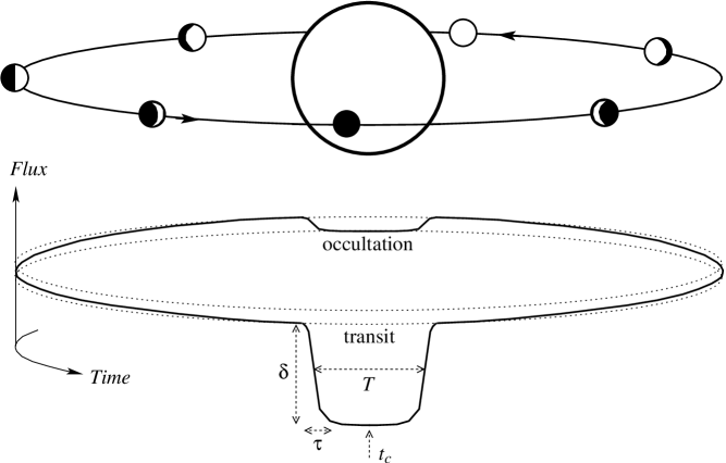
Figure 1: Illustration of transits and occultations. During a transit, the planet blocks a fraction of the starlight. Afterwards, the planet’s brighter dayside comes into view and the total flux rises. The total flux drops again when the planet is occulted by the star.

Table 1: Properties that have been measured, or that might be measured in the future, through precise observations of transiting planets.

Property	Refs.	Property	Refs.
Orbital period	1,2	Planet-planet interactions (short-term)	19,20
Orbital inclination	1,2	Planet-planet interactions (long-term)	21,22
Planetary mass	1,2	Mutual orbital inclinations	20,23
Planetary radius	1,2	Planetary rings	24,25
Stellar obliquity	3,4	Satellites	9,24
Orbital eccentricity	5,6	Relativistic precession	26,27
Stellar limb darkening	7	Parallax effects	28, 29
Star spots	8,9	Apsidal motion constant	30
Thermal emission	5,10	Stellar differential rotation	31
Absorption spectrum	11,12	Oblateness and obliquity	32,33
Albedo	13,14	Variations in stellar radius	34
Phase function	15	Yarkovsky effect	35
Effective radiative time constant	16	Planetary wind speed	36
Trojan companions	17,18	Artificial planet-sized objects	37

Non-exhaustive list of references: (1) Charbonneau et al. (2000). (2) Henry et al. (2000). (3) Queloz et al. (2000). (4) Winn et al. (2005). (5) Charbonneau et al. (2005). (6) Bakos et al. (2007). (7) Knutson et al. (2007a). (8) Silva (2003). (9) Pont et al. (2007). (10) Deming et al. (2005). (11) Charbonneau et al. (2002). (12) Vidal-Madjar et al. (2003). (13) Rowe et al. (2006). (14) Winn et al. (2008a). (15) Knutson et al. (2007b). (16) Langton & Laughlin (2008). (17) Ford & Gaudi (2006), (18) Madhusudhan & Winn (2008). (19) Holman & Murray (2005). (20) Agol et al. (2005). (21) Miralda-Escudé (2002). (22) Heyl & Gladman (2007). (23) Fabrycky, D., these proceedings. (24) Brown et al. (2001). (25) Barnes & Fortney (2004). (26) Pál & Kocsis (2008). (27) Jordan & Bakos (2008). (28) Scharf (2007). (29) Rafikov (2008). (30) Ragozzine & Wolf (2008). (31) Gaudi & Winn (2007). (32) Seager & Hui (2002), (33) Barnes & Fortney (2003). (34) Loeb (2008). (35) Fabrycky (2008). (36) Spiegel et al. (2007). (37) Arnold (2005).

Table 1 summarizes the information that has been obtained—or that is obtainable in principle—through precise observations of transits and occultations. This table is surely incomplete. Every few months, a new and creative application of transit observations is proposed. I was asked to discuss some of the measurements that can be made with the highest signal-to-noise ratio. In the best cases, we can measure orbital periods with 8 significant digits; transit times to within a fraction of a minute; the planetary mass and radius to within a few per cent; and the stellar obliquity (or at least its sky projection) to within a few degrees.

2 Transit light curve parameters

In any discussion of measuring accurate transit parameters, the first question should be: what are those parameters? Ignoring limb darkening for the moment, the 4 basic observables are (with reference to Fig. 1) the mid-transit time $t_{c}$, the depth $\delta$, the total duration $T$, and the partial duration $\tau$. These observables can be translated into 3 dimensionless parameters describing the physical properties of the system:

$${\rm Radius~{}ratio}~{} R_{p}/R_{s} \approx~{}\sqrt{\delta},$$ (1)

$${\rm Impact~{}parameter}~{} b \approx~{}1-\sqrt{\delta}\frac{T}{\tau},$$ (2)

$${\rm Scaled~{}stellar~{}radius}~{} R_{s}/a \approx~{}\frac{\pi\sqrt{T\tau}}{\delta^{1/4}P}\left(\frac{1+e\sin\omega}{\sqrt{1-e^{2}}}\right),$$ (3)

where $R_{p}$ and $R_{s}$ are the planetary and stellar radii; $b$ is the impact parameter; $P$ is the orbital period; and $e$ and $\omega$ are the orbital eccentricity and argument of pericenter, which can be measured from the Doppler data. The approximations given here are valid for small values of $\delta$, $\tau/T$, and $T/P$, and they neglect limb darkening. Some useful references are Seager & Mallen-Ornelas (2003), who give the exact correspondences for a circular orbit, and Carter et al. (2008), who derive analytic expressions for the errors in these quantities. Mandel & Agol (2002) and Gimenez (2006) provide codes for calculating realistic light curves including limb darkening.

The dimensionless parameters of Eqns. (2.1-2.3) are useful, but oftentimes one is more interested in dimensionful parameters such as the planetary mass in Jovian masses, or the semimajor axis in AU. For those, the light curve analysis must be supplemented with some external information, such as an estimate of the stellar mass and/or radius based on the stellar parallax, spectrum, angular diameter, and any other available data. Interestingly, though, if one is willing to trust Kepler’s Law, then the transit observables may be combined into two quantities with dimensions (Seager & Mallen-Ornelas 2003, Southworth et al. 2007):

$${\rm Stellar~{}mean~{}density}~{} \rho_{s} \approx~{}\frac{3P}{\pi^{2}G}\left(\frac{\sqrt{\delta}}{T\tau}\right)^{3/2}\left[\frac{1-e^{2}}{(1+e\sin\omega)^{2}}\right]^{3/2}$$ (4)

$${\rm Planetary~{}surface~{}gravity}~{} g_{p} \approx~{}\frac{2\pi K_{s}}{P}\frac{\sqrt{1-e^{2}}}{\delta(R_{s}/a)^{2}\sin i},$$ (5)

where $K_{s}$ is the velocity semi-amplitude of the stellar radial-velocity signal, and $i$ is the orbital inclination. The inclination can be written in terms of observables using

$$b=\frac{a\cos i}{R_{s}}\left(\frac{1-e^{2}}{1+e\sin\omega}\right).$$ (6)

Knowledge of the stellar mean density is helpful for pinning down the stellar properties. The photometrically-determined $\rho_{s}$ is superior as a gravity indicator than the traditional $\log g$ that is based on the widths of pressure-sensitive absorption lines (see, e.g., Sozzetti et al. 2007, Winn et al. 2008b). Recently, Torres et al. (2008) put this technique into practice for 23 transiting exoplanets, in the most homogeneous and complete analysis of transit data to date. A similar effort is underway by Southworth (2008). The relative immunity of $g_{p}$ to systematic errors in the stellar properties suggests that when testing theoretical models of planetary structure, it would be wiser to compare theoretical and observed surface gravities, rather than the traditional comparison between theoretical and observed radii.

Figure 2: A gallery of transit light curves based on observations with spaceborne instruments. The upper 3 panels show optical data from the Hubble Space Telescope  and the lower 3 panels show infrared data from the Spitzer Space Telescope.

This field has been blessed with spectacular data from the space observatories, some of which are shown in Fig. 2. Everyone remembers exactly where they were when they first saw the Hubble Space Telescope  (HST ) light curve of HD 209458 by Brown et al. (2001), with a cadence of 80 s and a precision of $1.1\times 10^{-4}$. This group established the protocol of most subsequent HST  observations: schedule several “visits” to achieve complete phase coverage of the event; disperse the starlight over many pixels to average over sensitivity variations and achieve a high duty cycle; sum all of the detected photons; and correct for instabilities due to the spacecraft orbit and detector.

With the Spitzer Space Telescope  the count rates are generally lower, but there are compensatory advantages: there is little limb-darkening at at mid-infrared wavelengths, and uninterrupted views of entire events are possible because the satellite is not in a low-earth orbit. A few noteworthy Spitzer results are the transit of GJ 436 (Gillon et al. 2007, Deming et al. 2007), the Neptune-sized planet about which we heard so much this week, and a recent light curve by Nutzman et al. (2008) of the very challenging target HD 149026, for which the transit depth is only a quarter of a percent.

Ground-based photometry still plays an important role. With a large claim on a small telescope, one can observe many more events than is feasible from space, build a large library of transit times, and respond more quickly to new discoveries. Furthermore, in many cases it has been possible with ground-based photometry to reach the regime in which the contribution to the parameter uncertainties due to photometric errors is comparable to the systematic errors arising from uncertainties in the stellar properties. Beyond this point, improved photometric precision gives steeply diminishing returns. The following discussion is informed by my experience with the Transit Light Curve project, which Matt Holman and I have undertaken (see Fig. 3). It should be emphasized, however, that spectacular ground-based photometry has been achieved by several other groups (see, e.g., Alonso et al. 2008, or Gillon, M. in these proceedings).

Figure 3: A gallery of transit light curves, based on observations with small ground-based telescopes. Each panel shows a time-averaged (100 s), composite light curve based on observations of multiple transits. The number of observed transits ranges from 2 (XO-1) to 11 (GJ 436).

The aspiring ground-based transit observer is well-advised to consult some of the classic papers on CCD differential ensemble photometry, including Gilliland & Brown (1988), Kjeldsen & Frandsen (1992), and Everett & Howell (2001). Some lessons from these authors, as applied to transit observations, are to ensure that calibration frames have negligible photon-counting noise; keep the pointing stable to within a few pixels to minimize the effects of pixel-to-pixel gain variations; and strive to observe at least 10 comparison stars bracketing the target star in brightness and color. Each instrument will have a sweet spot, a magnitude range for which a 1 min exposure gives $\sim$10 good comparison stars within the field of view. For TLC observations, employing the 1.2m telescope at the Fred L. Whipple Observatory and the Keplercam $23^{\prime}$ detector, this occurs at 11-12th magnitude. For brighter targets, defocusing is helpful to draw out the maximum exposure time (and thereby increase the duty cycle) and to hedge against pixel-to-pixel variations and seeing variations.

It is often advisable to use a long-wavelength bandpass, where extinction variations are smaller and the effects of stellar limb darkening are reduced. Smaller limb darkening leads to light curves with sharper corners and flatter bottoms, providing more statistical leverage on the parameters $t_{c}$, $R_{p}/R_{s}$, $b$, and $R_{s}/a$. To be concrete, Fig. 4 shows the results of calculations by Pál (2008), comparing the statistical error in those parameters as a function of the observing bandpass. All other things being equal, observing in $K$ as opposed to $u$ reduces the statistical error in $t_{c}$ by $\sim$15%, in $R_{s}/a$ or $b$ by $\sim$40%, and $R_{p}/R_{s}$ by $\sim$80%. Of course, there are other factors that affect the choice of bandpass, such as the count rate; the purpose of Fig. 4 is to isolate the effect of limb darkening.

Figure 4: The effect of limb-darkening on parameter errors, based on calculations by Pál  (2008). Imagine a planet with $R_{p}/R_{s}=R_{s}/a=0.1$ transits a Sun-like star with impact parameter $b$, and a light curve is obtained with $1.3\times 10^{-3}$ precision and 10 s cadence. Shown here is the relative error in the parameters $R_{p}/R_{s}$ (solid), $b$ (dashed), $a/R_{s}$ (dash-dotted), and $t_{c}$ (dotted), as a function of the observing bandpass. For redder bandpasses (to the right), the effect of limb-darkening is smaller and the parameter errors are decreased.

A primary goal of high-precision transit observations is to characterize the mass and radius of the planet. Figure 5 shows results from the current ensemble. When possible, the results were taken from the homogeneous analysis of Torres et al. (2008) mentioned previously, and otherwise from the most recent literature. Almost all of the planets seem to be gas giants, with radii 10-50% larger than that of Jupiter. A persistent theme in this field is that at least a few planets have radii that are “too large” by the standards of theoretical models of H-He giant planets, even after accounting for the intense stellar heating and selection effects (see Burrows et al. 2007 for a recent discussion). In the left panel, with logarithmic axes, one may appreciate that the Neptune-sized planet GJ 436 is “halfway” from the gas giants to Earthlike planets.

Figure 5: Masses and radii of transiting planets. The dotted lines are loci of constant mean density. Values for Jupiter, Saturn, Neptune, and Earth are also plotted, for comparison.

Another reason to observe transits is to measure precise mid-transit times. These data can be used to detect additional planets using the method of Holman & Murray (2005) and Agol et al. (2005): planet-planet gravitational forces cause slight modifications in the orbit of the transiting planet, which are revealed by a pattern of anomalies in a sequence of transit times. This technique is especially sensitive to planets in mean-motion resonance with the transiting planet. The acquisition of transit times is being pursued by a large number of groups, many of whom have presented results at this meeting. Dynamical analyses by Agol & Steffen (2007), Miller-Ricci et al. (2008), and others have not yet resulted in any secure detections, but in the best cases they have ruled out terrestrial-mass planets in the lowest-order resonances.

As another illustration of the extreme sensitivity to resonant orbits, consider GJ 436. Circumstantial evidence for a super-Earth in the 2:1 resonance with the transiting planet was presented by Ribas et al. (2008). Figure 6, produced by D. Fabrycky, shows some recently measured transit times for GJ 436 along with the timing variations that one expects from a 5 $M_{\oplus}$ planet in the 2:1 resonance (solid lines). The amplitude of the theoretical timing variations are $\sim$$10^{4}$ s, far out of the plotting range, and are strongly excluded by the data. The largest allowed body in that particular orbit is about 0.05 $M_{\oplus}$, or 4 Lunar masses (dotted lines).

One may also search for planets in 1:1 resonance: Trojan planets, residing at the L4/L5 points of the planet’s orbit. Ford & Gaudi (2006) showed that Trojans can be detected by seeking a difference between the observed transit time and the calculated transit time based only on the radial-velocity data. This technique was recently applied to 25 transiting systems, and did not result in any secure detections, although for GJ 436 it was possible to rule out Trojans of mass 2.5 $M_{\oplus}$ or larger (Madhusudhan & Winn 2008).

Figure 6: Transit timing residuals (observed $-$ calculated) for GJ 436, along with theoretical variations that would be expected due to a second planet in a 2:1 resonance, with a mass of 5 $M_{\oplus}$ (solid line) and 0.05 $M_{\oplus}$ (dotted line). Calculations and figure by D. Fabrycky.

3 The Rossiter-McLaughlin effect

The last parameter I will discuss is the stellar obliquity, or spin-orbit angle, defined as the angle between the angular momentum vectors of the rotating star and of the planetary orbit. The spin-orbit angle is a fundamental geometric property, and for this reason alone, it is worth seeking empirical constraints on $\psi$ whenever possible. In addition, it has recently been recognized that $\psi$ is a possible diagnostic of theories of planet migration. Migration via tidal interactions with a protoplanetary disk would probably result in a close spin-orbit alignment. Migration due to planet-planet scattering events, or Kozai cycles accompanied by tidal friction, would produce at least occasionally large misalignments (see, e.g., Fabrycky & Tremaine 2007, Wu et al. 2007, Chatterjee et al. 2008, Nagasawa et al. 2008, Juric & Tremaine 2008). Independently of the interpretation, one may regard $\psi$ to be on a par with the semimajor axis and the eccentricity: all are basic geometric parameters, for which accurate and systematic measurements can lead to revealing discoveries and statistical constraints on exoplanetary system architectures.

Alas, the spin-orbit angle is not generally measurable. However, by monitoring the apparent Doppler shift of the host star throughout a transit (in addition to the loss of light) one may determine the angle between the sky projections  of the two angular momentum vectors, which is denoted $\lambda$ and referred to as the projected spin-orbit angle. It is then possible to derive a lower limit on $\psi$ for an individual system, and to derive statistical constraints on $\psi$ from an ensemble of results.

The sensitivity to $\lambda$ arises from a spectroscopic phenomenon described by Rossiter (1924) and McLaughlin (1924) for the case of eclipsing binaries, and known today as the RM effect. During a transit, the planet blocks a portion of the rotating stellar surface, thereby hiding some of the velocity components that ordinarily contribute to the stellar line broadening. The result is a distorted line profile that is usually manifested as an “anomalous” Doppler shift. When the planet is projected in front of the approaching (blueshifted) half of the star, the net starlight appears slightly redshifted, and vice versa. Figure 7 shows three trajectories of a transiting planet that have the same impact parameter—and hence produce identical light curves—but that have different orientations relative to the stellar spin axis, and hence produce different RM signals. The signal for a well-aligned planet is antisymmetric about the midtransit time (left panels), whereas a strongly misaligned planet that spends all its time in front of the receding half of the star will produce only an anomalous blueshift (right panels).

Figure 7: The Rossiter-McLaughlin (RM) effect as an “anomalous” Doppler shift. Top: three possible transit geometries that produce identical light curves, but differ in spin-orbit alignment. Bottom: The corresponding radial-velocity signals. Dotted lines are for the idealized case of no limb darkening; solid lines include limb darkening.

Table 2: Results for the projected spin-orbit angle, $\lambda$.

System	$\lambda$ [deg]	Refs.
HD 189733	$-1.4\pm 1.1$	1
HD 209458	$-4.4\pm 1.4$	2,3⋆
HAT-P-1	$+3.6\pm 2.0$	4
CoRoT-Exo-2	$+7.2\pm 4.5$	5
HD 17156	$+9.4\pm 9.3$	6,7⋆
TrES-2	$-9\pm 12$	8
HAT-P-2	$+1\pm 13$	9⋆,10
HD 149026	$-12\pm 15$	11
XO-3	$+70\pm 15$	12
WASP-14	$-14\pm 17$	13
TrES-1	$+30\pm 21$	14

References: (1) Winn et al. (2006). (2) Queloz et al. (2000). (3) Winn et al. (2005). (4) Johnson et al. (2008). (5) Bouchy et al. (2008). (6) Narita et al. (2008). (7) Cochran et al. (2008). (8) Winn et al. (2008c). (9) Winn et al. (2007d). (10) Loeillet et al. (2008). (11) Wolf et al. (2007). (12) Hebrard et al. (2008). (13) Joshi et al. (2008). (14) Narita et al. (2007). Note: where more than one reference is listed, the value in column 2 is taken from the starred reference.

To date, RM observations have been reported for 11 different exoplanetary systems, since the pioneering detections by Queloz et al. (2000) and Bundy & Marcy (2000). This field is at the transition point between a mere handful of results to a large enough sample for meaningful general conclusions to be drawn and for rare surprises to emerge. The results are summarized in Table 2, which is organized in order of measurement precision, with the most precise result listed first. Figure 8 shows some more recent data for HD 189733 and HAT-P-2, both of which display the antisymmetric waveform indicative of a well-aligned spin and orbit (at least in projection). Both stars have candidate stellar companions, naturally raising the possibility of Kozai cycles, but in both cases the projected spin-orbit angle is consistent with zero.

Figure 8: Examples of RM data. The top panels show transit photometry, and the bottom panels show the corresponding radial-velocity waveform. The out-of-transit gradient in the radial velocity is due to the orbital motion of the star. The in-transit “blip” is the RM effect.

In almost all cases, the results are consistent with good alignment, with measurement precisions ranging from $1^{\circ}$ to $21^{\circ}$. There are two possible exceptions. The first is HD 17156, for which Narita et al. (2008) reported $\lambda=62^{\circ}\pm 25^{\circ}$. However, shortly after this meeting, Cochran et al. (2008) presented new data giving $9.4^{\circ}\pm 9.3^{\circ}$. The reason for the apparently significant disagreement between the data sets is not yet clear. The other possible exception is XO-3, for which Hébrard et al. (2008) found $\lambda=70^{\circ}\pm 15^{\circ}$ deg, i.e., a transverse RM effect in which only an anomalous blueshift was seen. Those authors expressed some caution about the result due to possible systematic errors. Further observations of both of these systems are warranted.

Broadly speaking, the results show that large spin-orbit misalignments are fairly rare. The time is now ripe for a statistical analysis of the ensemble results. This would not only overcome the sky-projection limitation that is inherent in individual results, but could ultimately place constraints on the fraction of systems that have migrated via different channels. A possible confounding factor is tidal coplanarization: even if the migration process resulted in a large value of $\psi$, could the system have been eventually realigned by star-planet tidal interactions? The simple and widely-used model of tidal interactions, in which the equilibrium tidal bulge is shifted by a constant time lag, suggests that the timescale for inclination damping is much longer than the timescale for eccentricity damping, and that tidal spin-orbit realignment can be neglected (Winn et al. 2005). However, more theoretical work is needed to go beyond this order-of-magnitude argument and define the scope for more complicated tidal and evolutionary models to affect the interpretation of the RM results. It is possible, for example, that tidal dynamics were more important when the system was younger, or that the coplanarization timescale is shorter than expected (Mazeh 2008).