SUSY GUT Model Building

Abstract

I discuss an evolution of SUSY GUT model building, starting with the construction of 4d GUTs, to orbifold GUTs and finally to orbifold GUTs within the heterotic string. This evolution is an attempt to obtain realistic string models, perhaps relevant for the LHC. This review is in memory of the sudden loss of Julius Wess, a leader in the field, who will be sorely missed.

1 Motivation

Before beginning this review on SUSY GUTs, it is probably worthwhile spending a very brief moment motivating the topic. What are the virtues of SUSY GUTs? The following is a list of all the issues that SUSY GUTs either addresses directly or provides a framework for addressing.

1. $M_{Z}<<M_{GUT}$ “Natural”

2. Explains Charge Quantization and family structure

3. Predicts Gauge Coupling Unification^∗

4. Predicts Yukawa Coupling Unification

5. + Family Symmetry $\Longrightarrow$ Hierarchy of Fermion Masses

6. Neutrino Masses via See - Saw scale $\sim 10^{-3}-10^{-2}\ M_{G}$

7. LSP – Dark Matter Candidate

8. Baryogenesis via Leptogenesis

9. SUSY Desert $\Longrightarrow$ LHC experiments probe
   physics O($M_{Planck}$) scale

10. SUSY GUTs are natural extension of the Standard Model

In the following review we will discuss some of these issues in great detail. Let us start by defining our notation for the Standard Model.

2 Standard Model

Let us define the generators for the gauge group $SU(3)\otimes SU(2)\otimes U(1)_{Y}$ as ${\cal T}_{A},\ A=1,\dots,8$ for $SU(3)$ , $T_{a},\ a=1,2,3$ for $SU(2)$ and the hypercharge operator $Y$ for $U(1)_{Y}$.

The gauge interactions of the quarks and leptons of the Standard Model are then completely defined in terms of their gauge quantum numbers. The quark and lepton fields for one family are given in terms of the left-handed Weyl spinors -

$$q=\left(\begin{array}[]{c}u\\ d\end{array}\right),\ u^{c},\ d^{c},l=\left(\begin{array}[]{c}\nu\\ e\end{array}\right),\ e^{c},\ \nu^{c}$$ (1)

with SM charges given by

$${\cal T}_{A}\ q=\frac{1}{2}\lambda_{A}\ q,\ {\cal T}_{A}\ u^{c}=-\frac{1}{2}\lambda_{A}^{T}\ u^{c},\ {\cal T}_{A}\ d^{c}=-\frac{1}{2}\lambda_{A}^{T}\ d^{c}$$

$${\cal T}_{A}\ l={\cal T}_{A}\ e^{c}={\cal T}_{A}\ \nu^{c}=0$$ (2)

(where $\lambda_{A}$ are the 3 $\times$ 3 Gell-Mann matrices).

$$T_{a}\ q=\frac{1}{2}\tau_{a}\ q,\ T_{a}\ l=\frac{1}{2}\tau_{a}\ l$$

$$T_{a}\ u^{c}=T_{a}\ d^{c}=T_{a}\ e^{c}=T_{a}\ \nu^{c}=0$$ (3)

(where $\tau_{a}$ are the 2 $\times$ 2 Pauli matrices).

$$Y\ q=\frac{1}{3}\ q,\ Y\ u^{c}=-\frac{4}{3}\ u^{c},\ Y\ d^{c}=\frac{2}{3}\ d^{c},$$

$$\ Y\ l=-l,\ Y\ e^{c}=+2e^{c},\ Y\ \nu^{c}=0.$$ (4)

With this notation, the gauge covariant derivative is given by

$$D_{\mu}=(\partial_{\mu}+ig_{s}{\cal T}_{A}{\cal G}_{\mu A}+igT_{a}W_{\mu a}+ig^{\prime}\ \frac{Y}{2}B_{\mu})$$ (5)

and the electric charge operator is given by $Q=T_{3}+\frac{Y}{2}$.

And the gauge-fermion Lagrangian is given by

$${\cal L}_{gauge-fermion}=[l^{*}\ i\bar{\sigma}_{\mu}D^{\mu}\ l+\cdots]+[-\frac{1}{2}Tr({\cal G}_{\mu\nu}{\cal G}^{\mu\nu})+\cdots].$$ (6)

In order to make contact with phenomenology it is sometimes useful to use Dirac four component notation. For example, the Dirac 4 component electron field, in terms of the 2 component Weyl spinors, is given by

$$\Psi_{e}=\left(\begin{array}[]{c}e\\ i\sigma_{2}\ (e^{c})^{*}\end{array}\right).$$ (7)

In addition we must add the Higgs bosons. We will introduce the minimal set of Higgs doublets consistent with supersymmetry.

$$H_{u}=\left(\begin{array}[]{c}h^{+}\\ h^{0}\end{array}\right),H_{d}=\left(\begin{array}[]{c}\bar{h}^{0}\\ \bar{h}^{-}\end{array}\right)$$ (8)

satisfying

$${\cal T}_{A}\ H_{u}={\cal T}_{A}\ H_{d}=0$$

$$T_{a}\ H_{u}=\frac{1}{2}\tau_{a}\ H_{u},\ T_{a}\ H_{d}=\frac{1}{2}\tau_{a}\ H_{d}$$

$$Y\ H_{u}=+H_{u},\ Y\ H_{d}=-H_{d}.$$ (9)

$$-{\cal L}_{Yukawa}= \lambda_{e}^{ij}\ l_{i}\ e^{c}_{j}\ H_{d}+\lambda_{d}^{ij}\ q_{i}\ d^{c}_{j}\ H_{d}+$$

$$\lambda_{u}^{ij}\ q_{i}\ u^{c}_{j}\ H_{u}+\lambda_{\nu}^{ij}\ l_{i}\ \nu^{c}_{j}\ H_{u}-\frac{1}{2}M_{ij}\ \nu^{c}_{i}\ \nu^{c}_{j}.$$

The generalization to the Minimal Supersymmetric Standard Model is then quite simple. One defines the left-handed chiral superfields. For example, the electron left-handed Weyl field, $e$, is contained in the left-handed chiral superfield, $E$, with

$$E(y,\theta)=\tilde{e}(y)+\sqrt{2}(\theta\ e(y))+(\theta\ \theta)F_{e}(y)$$ (11)

where the product $(\theta\ e(y))\equiv\theta^{\alpha}\ e(y)_{\alpha}$ and
$y^{\mu}=x^{\mu}-i\theta\ \sigma^{\mu}\theta^{*}$.

Then the supersymmetric Lagrangian includes the gauge-matter terms

$${\cal L}_{gauge-matter}=$$ (12)

$$[\int d^{4}\theta L_{i}^{\dagger}\ \exp(-2\ [g_{s}V_{g}+gV_{W}+g^{\prime}\frac{Y}{2}V_{B}])\ L_{i}+\cdots]$$

$$+[\frac{1}{8g_{s}^{2}}\int d^{2}\theta Tr({{\cal W}_{g}}^{\alpha}\ {{\cal W}_{g}}_{\alpha}+h.c.)+\cdots]$$

where $V_{g}=V_{A}\ {\cal T}_{A},\ V_{W}=V_{a}\ T_{a}$ and the flavor index $i=1,2,3$.

${\cal L}_{Yukawa}=\int d^{2}\theta W$ with the superpotential given by

$$W=$$ (13)

$$\lambda_{e}^{ij}\ L_{i}\ E^{c}_{j}\ H_{d}+\lambda_{d}^{ij}\ Q_{i}\ D^{c}_{j}\ H_{d}+\lambda_{u}^{ij}\ Q_{i}\ U^{c}_{j}\ H_{u}$$

$$+\lambda_{\nu}^{ij}\ L_{i}\ N^{c}_{j}\ H_{u}-\frac{1}{2}M_{ij}\ N^{c}_{i}\ N^{c}_{j}-\mu\ H_{u}\ H_{d}.$$

3 Two roads to Grand Unification

One can first unify quarks and leptons into two irreducible representations of the group $SU(4)_{C}\otimes SU(2)_{L}\otimes SU(2)_{R}$, i.e. the so-called Pati-Salam group ps where lepton number is the fourth color.

Then the PS fields

$${\cal Q}=(q\;l),\;{\cal Q}^{c}=(q^{c}\;l^{c})$$ (14)

where

$$q^{c}=\left(\begin{array}[]{c}u^{c}\\ d^{c}\end{array}\right),\;l^{c}=\left(\begin{array}[]{c}\nu^{c}\\ e^{c}\end{array}\right)$$ (15)

transform as $(4,2,1)\oplus(\bar{4},1,\bar{2})$ under PS. One can check that baryon number minus lepton number acting on a 4 of $SU(4)$ is given by

$$B-L=\left(\begin{array}[]{cccc}\frac{1}{3}&&&\\ &\frac{1}{3}&&\\ &&\frac{1}{3}&\\ &&&-1\end{array}\right)$$ (16)

and similarly electric charge is given by

$$Q=T_{3L}+T_{3R}+\frac{1}{2}(B-L).$$ (17)

Note, charge is quantized since it is embedded in a non-abelian gauge group. One family is contained in two irreducible representations. Finally, if we require parity ( $L\leftrightarrow R$ ) then there are two independent gauge couplings.

What about the Higgs? The two Higgs doublets $H_{u},\ H_{d}$ are combined into one irreducible PS Higgs multiplet

$${\cal H}=(H_{d}\ H_{u})$$ (18)

transforming as a $(1,2,\bar{2})$ under PS. Thus for one family, there is a unique renormalizable Yukawa coupling given by

$$\lambda\ {\cal Q}^{c}\ {\cal H}\ {\cal Q}$$ (19)

giving the GUT relation

$$\lambda_{t}=\lambda_{b}=\lambda_{\tau}=\lambda_{\nu_{\tau}}\equiv\lambda.$$ (20)

Now Pati-Salam is not a grand unified gauge group. However, since $SU(4)\approx SO(6)$ and $SU(2)\otimes SU(2)\approx SO(4)$ (where $\approx$ signifies a homomorphism), it is easy to see that PS $\approx SO(6)\otimes SO(4)\subset SO(10)$ SO(10) . In fact one family of quarks and leptons is contained in the spinor representation of $SO(10)$, i.e.

$$SO(10)\rightarrow SU(4)_{C}\otimes SU(2)_{L}\otimes SU(2)_{R}$$

$$16\rightarrow(4,2,1)\oplus(\bar{4},1,\bar{2}).$$ (21)

Hence by going to $SO(10)$ we have obtained quark-lepton unification ( one family contained in one spinor representation ) and gauge coupling unification (one gauge group) (see Table 1).

But I should mention that there are several possible breaking patterns for $SO(10)$.

$$SO(10) \rightarrow SU(4)_{C}\otimes SU(2)_{L}\otimes SU(2)_{R}$$

$$\rightarrow SU(5)\otimes U(1)_{X}$$

$$\rightarrow SU(5)^{\prime}\otimes U(1)_{X^{\prime}}$$

$$\rightarrow SU(3)_{C}\otimes U(1)_{(B-L)}\otimes SU(2)_{L}\otimes SU(2)_{R}.$$

In order to preserve a prediction for gauge couplings we would require the breaking pattern

$$SO(10)\rightarrow SM$$ (23)

or

$$SO(10)\rightarrow SU(5)\rightarrow SM.$$ (24)

$$\begin{array}[]{|l|c|c|c|}\hline\cr\vrule\lx@intercol\rm Grand\;\;Unification\;-\;SO(10)\hfil\lx@intercol\vrule\lx@intercol\\ \hline\cr{\rm State}&{\rm Y}&{\rm Color}&{\rm Weak}\\ &=\frac{2}{3}\Sigma({\rm C})-\Sigma({\rm W})&{\rm C\;spins}&{\rm W\;spins}\\ \hline\cr\hline\cr{\bf\bar{\nu}}&{0}&+\,+\,+&+\,+\\ \hline\cr\hline\cr{\bf\bar{e}}&{2}&+\,+\,+&-\,-\\ \hline\cr{\bf u_{r}}&&-\,+\,+&+\,-\\ {\bf d_{r}}&&-\,+\,+&-\,+\\ {\bf u_{b}}&{\frac{1}{3}}&+\,-\,+&+\,-\\ {\bf d_{b}}&&+\,-\,+&-\,+\\ {\bf u_{y}}&&+\,+\,-&+\,-\\ {\bf d_{y}}&&+\,+\,-&-\,+\\ \hline\cr{\bf\bar{u}_{r}}&&+\,-\,-&+\,+\\ {\bf\bar{u}_{b}}&{-\frac{4}{3}}&-\,+\,-&+\,+\\ {\bf\bar{u}_{y}}&&-\,-\,+&+\,+\\ \hline\cr\hline\cr{\bf\bar{d}_{r}}&&+\,-\,-&-\,-\\ {\bf\bar{d}_{b}}&{\frac{2}{3}}&-\,+\,-&-\,-\\ {\bf\bar{d}_{y}}&&-\,-\,+&-\,-\\ \hline\cr{\bf\nu}&{-1}&-\,-\,-&+\,-\\ {\bf e}&&-\,-\,-&-\,+\\ \hline\cr\end{array}$$

Table 1: Spinor representation of $SO(10)$ where this table explicitly represents the Cartan-Weyl weights for the states of one family of quarks and leptons. The double lines separate irreducible representations of $SU(5)$.

It will be convenient at times to work with the Georgi-Glashow GUT group $SU(5)$ gg . We have $16\rightarrow 10\oplus\bar{5}\oplus 1$. Let’s identify the quarks and leptons of one family directly. We define the group $SU(5)$ by

$$SU(5)=\{U|U=5\times 5\;{\rm complex\;matrix};U^{\dagger}U=1;\det U=1\}$$ (25)

and the fundamental representation $5^{\alpha},\ \alpha=1,\dots,5$ transforms as

$${5^{\prime}}^{\alpha}={U^{\alpha}}_{\beta}\ 5^{\beta}.$$ (26)

We represent the unitary matrix $U$ by

$$U=\exp(iT_{A}\ \omega_{A})$$ (27)

where $Tr(T_{A})=0,\ T_{A}^{\dagger}=T_{A}$, $A=1,\dots,24$ and
$[T_{A},\ T_{B}]=if_{ABC}\ T_{C}$ with $f_{ABC}$ the structure constants of $SU(5)$. Under an infinitesimal transformation, we have

$$\delta_{A}5^{\alpha}=i{(T_{A})^{\alpha}}_{\beta}\ 5^{\beta}\ \omega_{A}.$$ (28)

Let us now identify the $SU(3)\otimes SU(2)\otimes U(1)_{Y}$ subgroup of $SU(5)$. The $SU(3)$ subgroup is given by the generators

$$T_{A}=\left(\begin{array}[]{c|c}\frac{1}{2}\lambda_{A}&0\\ \hline\cr 0&0\end{array}\right),\;\;A=1,\dots,8.$$ (29)

And the $SU(2)$ subgroup is given by

$$T_{A}=\left(\begin{array}[]{c|c}0&0\\ \hline\cr 0&\frac{1}{2}\tau_{(A-20)}\end{array}\right),\;\;A=21,22,23.$$ (30)

The generators in $SU(5)/SU(3)\otimes SU(2)\otimes U(1)_{Y}$ are given by

$$T_{A},\ A=9,\dots,20.$$ (31)

These are 12 generators of the form

$$\left(\begin{array}[]{c|c}0&\begin{array}[]{cc}1&0\\ 0&0\\ 0&0\end{array}\\ \hline\cr\begin{array}[]{ccc}1&0&0\\ 0&0&0\end{array}&0\end{array}\right),\;\;\left(\begin{array}[]{c|c}0&\begin{array}[]{cc}-i&0\\ 0&0\\ 0&0\end{array}\\ \hline\cr\begin{array}[]{ccc}i&0&0\\ 0&0&0\end{array}&0\end{array}\right).$$ (32)

Let us now identify the hypercharge $Y$. The only remaining generator of $SU(5)$ commuting with the generators of $SU(3)$ and $SU(2)$ is given by

$$T_{24}=\sqrt{\frac{3}{5}}\left(\begin{array}[]{c|c}\begin{array}[]{ccc}-1/3&0&0\\ 0&-1/3&0\\ 0&0&-1/3\end{array}&0\\ \hline\cr 0&\begin{array}[]{cc}1/2&0\\ 0&1/2\end{array}\end{array}\right)\equiv\sqrt{\frac{3}{5}}\ \frac{Y}{2}.$$ (33)

The overall normalization is chosen so that all the $SU(5)$ generators satisfy $Tr(T_{A}\ T_{B})=\frac{1}{2}\ \delta_{AB}.$

With these identifications, we see that the quantum numbers of a

$$5^{\alpha}=\left(\begin{array}[]{c}d^{a}\\ l^{i}\end{array}\right),\;a=1,2,3;i=4,5$$ (34)

where $d^{a}$ transforms as $(3,1,-2/3)$ and $l^{i}$ transforms as $(1,2,+1)$ under the SM. Of course these are not correct quantum numbers for any of the quarks and leptons, but the charge conjugate states are just right. We have

$$\bar{5}_{\alpha}=\left(\begin{array}[]{c}d^{c}_{a}\\ l^{c}_{i}\end{array}\right),\;a=1,2,3;i=4,5$$ (35)

with transformation properties

$$d^{c}=(\bar{3},1,2/3),\;\;l^{c}=(1,2,-1)$$ (36)

and

$$l^{c}=\left(\begin{array}[]{c}-e\\ \nu\end{array}\right).$$ (37)

Once we have identified the states of the $\bar{5}$, we have no more freedom for the $10$. The $10$ transforms as an anti-symmetric tensor product of two $5$s, i.e.

$$10^{\alpha\beta}=-10^{\beta\alpha}\propto 5_{1}^{\alpha}\ 5_{2}^{\beta}-5_{2}^{\alpha}\ 5_{1}^{\beta}.$$ (38)

We find

$$10^{ab}\equiv\epsilon^{abc}(u^{c})_{c}=(\bar{3},1,-4/3)$$

$$10^{ai}\equiv q^{ai}=(3,2,1/3)$$

$$10^{ij}\equiv\epsilon^{ij}e^{c}=(1,1,+2).$$ (39)

To summarize we find

$$\bar{5}_{\alpha}=\left(\begin{array}[]{c}d^{c}_{1}\\ d^{c}_{2}\\ d^{c}_{3}\\ -e\\ \nu\end{array}\right),\;\;10^{\alpha\beta}=\frac{1}{\sqrt{2}}\ \left(\begin{array}[]{c|c}\begin{array}[]{ccc}0&u^{c}_{3}&-u^{c}_{2}\\ -u^{c}_{3}&0&u^{c}_{1}\\ u^{c}_{2}&-u^{c}_{1}&0\end{array}&\begin{array}[]{cc}u^{1}&d^{1}\\ u^{2}&d^{2}\\ u^{3}&d^{3}\end{array}\\ \hline\cr\begin{array}[]{ccc}-u^{1}&-u^{2}&-u^{3}\\ -d^{1}&-d^{2}&-d^{3}\end{array}&\begin{array}[]{cc}0&e^{c}\\ -e^{c}&0\end{array}\end{array}\right).$$ (40)

Now that we have identified the states of one family in $SU(5)$, let us exhibit the fermion Lagrangian (with gauge interactions). We have

$${\cal L}_{fermion}=\bar{5}_{\alpha}^{\dagger}i(\bar{\sigma}_{\mu}\ {D^{\mu})_{\alpha}}^{\beta}\ \bar{5}_{\beta}+{10^{\alpha\beta}}^{\dagger}i(\bar{\sigma}_{\mu}\ D^{\mu})^{\alpha\beta}_{\gamma\delta}\ 10^{\gamma\delta}$$ (41)

where

$$D^{\mu}=\partial^{\mu}+ig_{G}T_{A}\ A^{\mu}_{A}$$ (42)

and $T_{A}$ is in the $\bar{5}$ or $10$ representation. We see that since there is only one gauge coupling constant at the GUT scale we have

$$g_{3}=g_{2}=g_{1}\equiv g_{G}$$ (43)

where, after weak scale threshold corrections are included, we have

$$g_{3}\rightarrow g_{s},\;g_{2}\rightarrow g,\;g_{1}\rightarrow\sqrt{\frac{5}{3}}\ g^{\prime}.$$ (44)

At the GUT scale we have the relation

$$\sin^{2}\theta_{W}=\frac{(g^{\prime})^{2}}{g^{2}+(g^{\prime})^{2}}=3/8.$$ (45)

But these are tree level relations which do not take into account threshold corrections at either the GUT or the weak scales nor renormalization group [RG] running from the GUT scale to the weak scale. Consider first RG running. The one loop RG equations are given by

$$\frac{d\alpha_{i}}{dt}=-\frac{b_{i}}{2\pi}\alpha_{i}^{2}$$ (46)

where $\alpha_{i}=\frac{g_{i}^{2}}{4\pi},\;i=1,2,3$ and

$$b_{i}=\frac{11}{3}C_{2}(G_{i})-\frac{2}{3}T_{R}\ N_{F}-\frac{1}{3}T_{R}\ N_{S}.$$ (47)

Note, $t=-\ln(\frac{M_{G}}{\mu})$, $\sum_{A}(T_{A}^{2})=C_{2}(G_{i})\mathbb{I}$ with $T_{A}$ in the adjoint representation defines the quadratic Casimir for the group $G_{i}$ with $C_{2}(SU(N))=N$ and $C_{2}(U(1))=0$. $Tr(T_{A}T_{B})=T_{R}\ \delta_{AB}$ for $T_{A}$ in the representation $R$ (for $U(1)_{Y}$, $T_{R}\equiv\frac{3}{5}\ Tr(\frac{Y^{2}}{4})$) and $N_{F}(N_{S})$ is the number of Weyl fermions (complex scalars) in representation $R$. For N = 1 supersymmetric theories, Equation 47 can be made more compact. We have

$$b_{i}=3C_{2}(G_{i})-T_{R}\ N_{\chi}$$ (48)

where the first term takes into account the vector multiplets and $N_{\chi}$ is the number of left-handed chiral multiplets in the representation $R$ drw ; 2loop . The solution to the one loop RG equations is given by

$$\alpha_{i}(M_{Z})^{-1}=\alpha_{G}^{-1}-\frac{b_{i}}{2\pi}\ln(\frac{M_{G}}{M_{Z}}).$$ (49)

For the SM we find

$${\bf b}_{SM}\equiv(b_{1},b_{2},b_{3})$$ (50)

$$=(-\frac{4}{3}N_{fam}-\frac{1}{10}N_{H},\frac{22}{3}-\frac{4}{3}N_{fam}-\frac{1}{6}N_{H},11-\frac{4}{3}N_{fam})$$

where $N_{fam}(N_{H})$ is the number of families (Higgs doublets). For SUSY we have

$${\bf b}_{SUSY}=$$ (51)

$$=(-2N_{fam}-\frac{3}{5}N_{(H_{u}+H_{d})},6-2N_{fam}-N_{(H_{u}+H_{d})},9-2N_{fam})$$

where $N_{(H_{u}+H_{d})}$ is the number of pairs of Higgs doublets. Thus for the MSSM we have

$${\bf b}^{MSSM}=(-33/5,-1,3).$$ (52)

The one loop equations can be solved for the value of the GUT scale $M_{G}$ and $\alpha_{G}$ in terms of the values of $\alpha_{EM}(M_{Z})$ and $\sin^{2}\theta_{W}(M_{Z})$. We have (without including weak scale threshold corrections)

$$\alpha_{2}(M_{Z})=\frac{\alpha_{EM}(M_{Z})}{\sin^{2}\theta_{W}(M_{Z})},\;\alpha_{1}(M_{Z})=\frac{\frac{5}{3}\alpha_{EM}(M_{Z})}{\cos^{2}\theta_{W}(M_{Z})}$$ (53)

and we find

$$(\frac{3}{5}-\frac{8}{5}\ \sin^{2}\theta_{W}(M_{Z}))\alpha_{EM}(M_{Z})^{-1}=(\frac{b^{MSSM}_{2}-b^{MSSM}_{1}}{2\pi})\ln(\frac{M_{G}}{M_{Z}})$$ (54)

which we use to solve for $M_{G}$. Then we use

$$\alpha_{G}^{-1}=\sin^{2}\theta_{W}(M_{Z})\ \alpha_{EM}(M_{Z})^{-1}+\frac{b^{MSSM}_{2}}{2\pi}\ln(\frac{M_{G}}{M_{Z}})$$ (55)

to solve for $\alpha_{G}$. We can then predict the value for the strong coupling using

$$\alpha_{3}(M_{Z})^{-1}=\alpha_{G}^{-1}-\frac{b^{MSSM}_{3}}{2\pi}\ln(\frac{M_{G}}{M_{Z}}).$$ (56)

Given the experimental values $\sin^{2}\theta_{W}(M_{Z})\approx.23$ and $\alpha_{EM}(M_{Z})^{-1}\approx 128$ we find $M_{G}\approx 1.3\times 10^{13}$ GeV with $N_{H}=1$ and $\alpha_{G}^{-1}\approx 42$ for the SM with the one loop prediction for $\alpha_{3}(M_{Z})\approx 0.07$. On the other hand, for SUSY we find $M_{G}\approx 2.7\times 10^{16}$ GeV, $\alpha_{G}^{-1}\approx 24$ and the predicted strong coupling $\alpha_{3}(M_{Z})\approx 0.12$. How well does this agree with the data? According to the PDG the average value of $\alpha_{s}(M_{Z})=0.1176\pm 0.002$ pdg . So at one loop the MSSM is quite good, while non-SUSY GUTs are clearly excluded.

At the present date, the MSSM is compared to the data using 2 loop RG running from the weak to the GUT scale with one loop threshold corrections included at the weak scale. These latter corrections have small contributions from integrating out the W, Z, and top quark. But the major contribution comes from integrating out the presumed SUSY spectrum. With a “typical” SUSY spectrum and assuming no threshold corrections at the GUT scale, one finds a value for $\alpha_{s}(M_{Z})\geq 0.127$ which is too large Langacker:1995fk . It is easy to see where this comes from using the approximate analytic formula

$$\alpha_{i}^{-1}(M_{Z})=\alpha_{G}^{-1}-\frac{b^{MSSM}_{i}}{2\pi}\ln(\frac{M_{G}}{M_{Z}})+\delta_{i}$$ (57)

where

$$\delta_{i}=\delta_{i}^{h}+\delta_{i}^{2}+\delta_{i}^{l}.$$ (58)

The constants $\delta_{i}^{2},\ \delta_{i}^{l},\ \delta_{i}^{h}$ represent the 2 loop running effects 2loop , the weak scale threshold corrections and the GUT scale threshold corrections, respectively. We have

$$\delta_{i}^{2}\approx-\frac{1}{\pi}\sum_{j=1}^{3}\frac{b^{MSSM}_{ij}}{b^{MSSM}_{j}}\log\left[1-b^{MSSM}_{j}\left(\frac{3-8\sin^{2}\theta_{W}}{36\sin^{2}\theta_{W}-3}\right)\right]$$ (59)

where the matrix $b^{MSSM}_{ij}$ is given by 2loop

$$b^{MSSM}_{ij}=\left(\begin{array}[]{ccc}\frac{199}{100}&\frac{27}{20}&\frac{22}{5}\\ \frac{9}{20}&\frac{25}{4}&6\\ \frac{11}{20}&\frac{9}{4}&\frac{7}{2}\end{array}\right).$$ (60)

The light thresholds are given by

$$\delta_{i}^{l}=\frac{1}{\pi}\sum_{j}{b^{l}_{i}}(j)\log(\frac{m_{j}}{M_{Z}})$$ (61)

where the sum runs over all states at the weak scale including the top, $W$, Higgs and the supersymmetric spectrum. Finally the GUT scale threshold correction is given by

$$\delta_{i}^{h}=-\frac{1}{2\pi}\sum_{\zeta}b_{i}^{\zeta}\log(\frac{M_{\zeta}}{M_{G}}).$$ (62)

In general the prediction for $\alpha_{3}(M_{Z})$ is given by

$$\alpha_{3}^{-1}(M_{Z})= (\frac{b_{3}-b_{1}}{b_{2}-b_{1}})\alpha_{2}^{-1}(M_{Z})-(\frac{b_{3}-b_{2}}{b_{2}-b_{1}})\alpha_{1}^{-1}(M_{Z})$$

$$+(\frac{b_{3}-b_{2}}{b_{2}-b_{1}})\delta_{1}-(\frac{b_{3}-b_{1}}{b_{2}-b_{1}})\delta_{2}+\delta_{3}$$

$$= \frac{12}{7}\alpha_{2}^{-1}(M_{Z})-\frac{5}{7}\alpha_{1}^{-1}(M_{Z})$$ (63)

$$+\frac{1}{7}(5\delta_{1}-12\delta_{2}+7\delta_{3})$$

$$\equiv(\alpha_{3}^{LO})^{-1}+\delta_{s}$$

where $b_{i}\equiv b^{MSSM}_{i}$, $\alpha_{3}^{LO}(M_{Z})$ is the leading order one-loop result and $\delta_{s}\equiv\frac{1}{7}(5\delta_{1}-12\delta_{2}+7\delta_{3})$. We find $\delta_{s}^{2}\approx-0.82$ (Ref. Alciati:2005ur ) and $\delta_{s}^{l}=-0.04+\frac{19}{28\pi}\ln(\frac{T_{SUSY}}{M_{Z}})$ where the first term takes into account the contribution of the $W$, top and the correction from switching from the $\overline{MS}$ to $\overline{DR}$ RG schemes and (following Ref. Carena:1993ag )

$$T_{SUSY}=m_{\tilde{H}}(\frac{m_{\tilde{W}}}{m_{\tilde{g}}})^{28/19}\left[(\frac{m_{\tilde{l}}}{m_{\tilde{q}}})^{3/19}(\frac{m_{H}}{m_{\tilde{H}}})^{3/19}(\frac{m_{\tilde{W}}}{m_{\tilde{H}}})^{4/19}\right].$$ (64)

For a Higgsino mass $m_{\tilde{H}}=400$ GeV, a Wino mass $m_{\tilde{W}}=300$ GeV, a gluino mass $m_{\tilde{g}}=900$ GeV and all other mass ratios of order one, we find $\delta_{s}^{l}\approx-0.12$. If we assume $\delta_{s}^{h}=0$, we find the predicted value of $\alpha_{3}(M_{Z})=0.135$. In order to obtain a reasonable value of $\alpha_{3}(M_{Z})$ with only weak scale threshold corrections, we need $\delta_{s}^{2}+\delta_{s}^{l}\approx 0$ corresponding to a value of $T_{SUSY}\sim 5$ TeV. But this is very difficult considering the weak dependence $T_{SUSY}$ (Eqn. 64) has on squark and slepton masses. Thus in order to have $\delta_{s}\approx 0$ we need a GUT scale threshold correction

$$\delta_{s}^{h}\approx+0.94.$$ (65)

At the GUT scale we have

$$\alpha_{i}^{-1}(M_{G})=\alpha_{G}^{-1}+\delta_{i}^{h}.$$ (66)

Define

$$\tilde{\alpha}_{G}^{-1}=\frac{1}{7}[12\alpha_{2}^{-1}(M_{G})-5\alpha_{1}^{-1}(M_{G})]$$ (67)

(or if the GUT scale is defined at the point where $\alpha_{1}$ and $\alpha_{2}$ intersect, then $\tilde{\alpha}_{G}\equiv\alpha_{1}(M_{G})=\alpha_{2}(M_{G})$. Hence, in order to fit the data, we need a GUT threshold correction

$$\epsilon_{3}\equiv\frac{\alpha_{3}(M_{G})-\tilde{\alpha}_{G}}{\tilde{\alpha}_{G}}=-\tilde{\alpha}_{G}\ \delta_{s}^{h}\approx-4\%.$$ (68)

3.1 Nucleon Decay

Baryon number is necessarily violated in any GUT grs . In $SU(5)$ nucleons decay via the exchange of gauge bosons with GUT scale masses, resulting in dimension 6 baryon number violating operators suppressed by $(1/M_{G}^{2})$. The nucleon lifetime is calculable and given by
$\tau_{N}\propto M_{G}^{4}/(\alpha_{G}^{2}\;m_{p}^{5})$. The dominant decay mode of the proton (and the baryon violating decay mode of the neutron), via gauge exchange, is $p\rightarrow e^{+}\;\pi^{0}$ ($n\rightarrow e^{+}\;\pi^{-}$). In any simple gauge symmetry, with one universal GUT coupling and scale ($\alpha_{G},\;M_{G}$), the nucleon lifetime from gauge exchange is calculable. Hence, the GUT scale may be directly observed via the extremely rare decay of the nucleon. In SUSY GUTs, the GUT scale is of order $3\times 10^{16}$ GeV, as compared to the GUT scale in non-SUSY GUTs which is of order $10^{15}$ GeV. Hence the dimension 6 baryon violating operators are significantly suppressed in SUSY GUTs drw with $\tau_{p}\sim 10^{34-38}$ yrs.

However, in SUSY GUTs there are additional sources for baryon number violation – dimension 4 and 5 operators bviol . Although our notation does not change, when discussing SUSY GUTs all fields are implicitly bosonic superfields and the operators considered are the so-called F terms which contain two fermionic components and the rest scalars or products of scalars. Within the context of $SU(5)$ the dimension 4 and 5 operators have the form $({\bf 10\;\bar{5}\;\bar{5}})$ $\supset(U^{c}\;D^{c}\;D^{c})+(Q\;L\;D^{c})+(E^{c}\;L\;L)$ and $({\bf 10\;10\;10\;\bar{5}})$ $\supset(Q\;Q\;Q\;L)+(U^{c}\;U^{c}\;D^{c}\;E^{c})\;+$ $B$ and $L$ conserving terms, respectively. The dimension 4 operators are renormalizable with dimensionless couplings; similar to Yukawa couplings. On the other hand, the dimension 5 operators have a dimensionful coupling of order ($1/M_{G}$).

The dimension 4 operators violate baryon number or lepton number, respectively, but not both. The nucleon lifetime is extremely short if both types of dimension 4 operators are present in the low energy theory. However both types can be eliminated by requiring R parity. In $SU(5)$ the Higgs doublets reside in a ${\bf 5_{H},\;\bar{5}_{H}}$ and R parity distinguishes the ${\bf\bar{5}}$ (quarks and leptons) from ${\bf\bar{5}_{H}}$ (Higgs). R parity rparity (or its cousin, family reflection symmetry (see Dimopoulos and Georgi drw and DRW  drw2 ) takes $F\rightarrow-F,\;H\rightarrow H$ with $F=\{{\bf 10,\;\bar{5}}\},\;H=\{{\bf\bar{5}_{H},\;5_{H}}\}$. This forbids the dimension 4 operator $({\bf 10\;\bar{5}\;\bar{5}})$, but allows the Yukawa couplings of the form $({\bf 10\;\bar{5}\;\bar{5}_{H}})$ and $({\bf 10\;10\;5_{H}})$. It also forbids the dimension 3, lepton number violating, operator $({\bf\bar{5}\;5_{H}})$ $\supset(L\;H_{u})$ with a coefficient with dimensions of mass which, like the $\mu$ parameter, could be of order the weak scale and the dimension 5, baryon number violating, operator $({\bf 10\;10\;10\;\bar{5}_{H}})$ $\supset(Q\;Q\;Q\;H_{d})+\cdots$.

Note, in the MSSM it is possible to retain R parity violating operators at low energy as long as they violate either baryon number or lepton number only but not both. Such schemes are natural if one assumes a low energy symmetry, such as lepton number, baryon number or a baryon parity ir . However these symmetries cannot be embedded in a GUT. Thus, in a SUSY GUT, only R parity can prevent unwanted dimension four operators. Hence, by naturalness arguments, R parity must be a symmetry in the effective low energy theory of any SUSY GUT. This does not mean to say that R parity is guaranteed to be satisfied in any GUT.

Note also, R parity distinguishes Higgs multiplets from ordinary families. In $SU(5)$, Higgs and quark/lepton multiplets have identical quantum numbers; while in $E(6)$, Higgs and families are unified within the fundamental ${\bf 27}$ representation. Only in SO(10) are Higgs and ordinary families distinguished by their gauge quantum numbers. Moreover the $\mathbb{Z}_{4}$ center of $SO(10)$ distinguishes ${\bf 10}$s from ${\bf 16}$s and can be associated with R parity senjanovic .

Dimension 5 baryon number violating operators may be forbidden at tree level by symmetries in $SU(5)$, etc. These symmetries are typically broken however by the VEVs responsible for the color triplet Higgs masses. Consequently these dimension 5 operators are generically generated via color triplet Higgsino exchange. Hence, the color triplet partners of Higgs doublets must necessarily obtain mass of order the GUT scale. The dominant decay modes from dimension 5 operators are $p\rightarrow K^{+}\;\bar{\nu}\;\;(n\rightarrow K^{0}\;\bar{\nu})$. This is due to a simple symmetry argument; the operators $(Q_{i}\;Q_{j}\;Q_{k}\;L_{l}),\;\;(U^{c}_{i}\;U^{c}_{j}\;D^{c}_{k}\;E^{c}_{l})$ (where $i,\;j,\;k,\;l=1,2,3$ are family indices and color and weak indices are implicit) must be invariant under $SU(3)_{C}$ and $SU(2)_{L}$. As a result their color and weak doublet indices must be anti-symmetrized. However since these operators are given by bosonic superfields, they must be totally symmetric under interchange of all indices. Thus the first operator vanishes for $i=j=k$ and the second vanishes for $i=j$. Hence a second or third generation particle must appear in the final state drw2 .

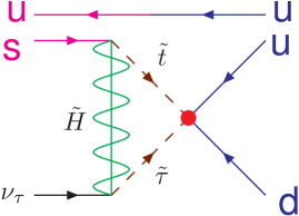
Figure 1: The effective four fermi operator for proton decay obtained by integrating out sparticles at the weak scale.

The dimension 5 operator contribution to proton decay requires a sparticle loop at the SUSY scale to reproduce an effective dimension 6 four fermi operator for proton decay (see Fig. 1). The loop factor is of the form

$$(LF)\propto\frac{\lambda_{t}\;\lambda_{\tau}}{16\pi^{2}}\frac{\sqrt{\mu^{2}+M_{1/2}^{2}}}{m_{16}^{2}}$$ (69)

leading to a decay amplitude

$$A(p\rightarrow K^{+}\bar{\nu})\propto\frac{c\ c}{M_{T}^{eff}}\ (\rm LF).$$ (70)

In any predictive SUSY GUT, the coefficients $c$ are 3 $\times$ 3 matrices related to (but not identical to) Yukawa matrices. Thus these tend to suppress the proton decay amplitude. However this is typically not sufficient to be consistent with the experimental bounds on the proton lifetime. Thus it is also necessary to minimize the loop factor, (LF). This can be accomplished by taking $\mu,M_{1/2}$ small and $m_{16}$ large. Finally the effective Higgs color triplet mass $M_{T}^{eff}$ must be MAXIMIZED. With these caveats, it is possible to obtain rough theoretical bounds on the proton lifetime given by Lucas:1995ic ; Altarelli:2000fu ; dmr

$$\tau_{p\rightarrow K^{+}\bar{\nu}}\leq(\frac{1}{3}-3)\times 10^{34}\;{\rm yrs.}.$$ (71)

3.2 Gauge Coupling Unification and Proton Decay

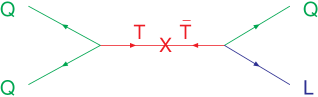
Figure 2: The effective dimension 5 operator for proton decay.

The dimension 5 operator (see Fig. 2) is given in terms of the matrices $c$ and an effective Higgs triplet mass by

$$\frac{1}{M^{eff}_{T}}\left[\ Q\ \frac{1}{2}\ c_{qq}Q\ Q\ c_{ql}L+\overline{U}\ c_{ud}\overline{D}\ \overline{U}\ c_{ue}\overline{E}\ \right].$$ (72)

Note, $M^{eff}_{T}$ can be much greater than $M_{G}$ without fine-tuning and without having any particle with mass greater than the GUT scale. Consider a theory with two pairs of Higgs $5_{i}$ and $\bar{5}_{i}$ with $i=1,2$ at the GUT scale with only $5_{1},\ \bar{5}_{1}$ coupling to quarks and leptons. Then we have

$$\frac{1}{M^{eff}_{T}}=(M_{T}^{-1})_{11}.$$ (73)

If the Higgs color triplet mass matrix is given by

$$M_{T}=\left(\begin{array}[]{cc}0&M_{G}\\ M_{G}&X\end{array}\right)$$ (74)

then we have

$$\frac{1}{M^{eff}_{T}}\equiv\frac{X}{M_{G}^{2}}.$$ (75)

Thus for $X<<M_{G}$ we obtain $M^{eff}_{T}>>M_{G}$.

We assume that the Higgs doublet mass matrix, on the other hand, is of the form

$$M_{D}=\left(\begin{array}[]{cc}0&0\\ 0&X\end{array}\right)$$ (76)

with two light Higgs doublets. Note this mechanism is natural in $S0(10)$ Dimopoulos:1981xm ; Babu:1993we with a superpotential of the form

$$W\supset 10\ 45\ 10^{\prime}+X\ (10^{\prime})^{2}$$ (77)

with only $10$ coupling to quarks and leptons, $X$ is a gauge singlet and $\langle 45\rangle=(B-L)\ M_{G}$.

Recall $\epsilon_{3}\equiv\frac{(\alpha_{3}(M_{G})-\tilde{\alpha}_{G})}{\tilde{\alpha}_{G}}\sim-4\%$. At one loop we find

$$\epsilon_{3}=\epsilon_{3}^{\rm Higgs}+\epsilon_{3}^{\rm GUT\;breaking}+\cdots.$$ (78)

Moreover

$$\epsilon_{3}^{\rm Higgs}=\frac{3\alpha_{G}}{5\pi}\ln(\frac{M^{eff}_{T}}{M_{G}}).$$ (79)

See Table 2 for the contribution to $\epsilon_{3}$ in Minimal SUSY $SU(5)$, and in an $SU(5)$ and $SO(10)$ model with natural Higgs doublet-triplet splitting.

Table 2: Contribution to $\epsilon_{3}$ in three different GUT models.

$$\begin{array}[]{|l|c|c|c|}\hline\cr{\rm Model}&{\rm Minimal}&{SU_{5}}&{\rm Minimal}\\ &SU_{5}&{\rm``Natural"D/T}\mbox{\cite[cite]{\@@bibref{Authors Phrase1YearPhrase2}{Altarelli:2000fu}{\@@citephrase{(}}{\@@citephrase{)}}}}&SO_{10}\mbox{\cite[cite]{\@@bibref{Authors Phrase1YearPhrase2}{dmr}{\@@citephrase{(}}{\@@citephrase{)}}}}\\ \hline\cr\epsilon_{3}^{\rm GUTbreaking}&0&-7.7\%&-10\%\\ \epsilon_{3}^{\rm Higgs}&-4\%&+3.7\%&+6\%\\ \hline\cr M^{eff}_{T}{\rm[GeV]}&2\times 10^{14}&3\times 10^{18}&6\times 10^{19}\\ \hline\cr\end{array}$$

Recent Super-Kamiokande bounds on the proton lifetime severely constrain these dimension 6 and 5 operators with $\tau_{(p\rightarrow e^{+}\pi^{0})}>8.0\times 10^{33}$ yrs susy08 , and $\tau_{(p\rightarrow K^{+}\bar{\nu})}>2.3\times 10^{33}$ yrs (92 ktyr) at (90% CL) based on the listed exposures superk . These constraints are now sufficient to rule out minimal SUSY $SU(5)$ murayama . The upper bound on the proton lifetime from these theories (particularly from dimension 5 operators) is approximately a factor of 5 above the experimental bounds. These theories are also being pushed to their theoretical limits. Hence if SUSY GUTs are correct, then nucleon decay must be seen soon.

3.3 Yukawa coupling unification

3.3.1 3rd generation, $b-\tau$ or $t-b-\tau$ unification

In $SU(5)$, there are two independent renormalizable Yukawa interactions given by $\lambda_{t}\;({\bf 10\;10\;5_{H}})$ $+\;\lambda\;({\bf 10\;\bar{5}\;\bar{5}_{H}})$. These contain the SM interactions $\lambda_{t}\;({\bf Q\;u^{c}\;H_{u}})$ $+\;\lambda\;({\bf Q\;d^{c}\;H_{d}}\;+\;{\bf e^{c}\;L\;H_{d}})$. Hence, at the GUT scale we have the tree level relation, $\lambda_{b}=\lambda_{\tau}\equiv\lambda$ chanowitz . In $SO(10)$ (or Pati-Salam) there is only one independent renormalizable Yukawa interaction given by $\lambda\;({\bf 16\;16\;10_{H}})$ which gives the tree level relation, $\lambda_{t}=\lambda_{b}=\lambda_{\tau}\equiv\lambda$ so10yuk ; hrr ; so10yuksusy . Note, in the discussion above we assume the minimal Higgs content with Higgs in ${\bf 5,\;\bar{5}}$ for $SU(5)$ and ${\bf 10}$ for $SO(10)$. With Higgs in higher dimensional representations there are more possible Yukawa couplings Lazarides:1980nt ; Bajc:2002iw ; Goh:2003sy .

In order to make contact with the data, one now renormalizes the top, bottom and $\tau$ Yukawa couplings, using two loop RG equations, from $M_{G}$ to $M_{Z}$. One then obtains the running quark masses $m_{t}(M_{Z})\;=\;\lambda_{t}(M_{Z})\;v_{u}$, $\;\;m_{b}(M_{Z})\;=\;\lambda_{b}(M_{Z})\;v_{d}$ and $\;m_{\tau}(M_{Z})\;=\;\lambda_{\tau}(M_{Z})\;v_{d}$ where $<H_{u}^{0}>\equiv v_{u}=\sin\beta\;v/\sqrt{2}$, $<H_{d}^{0}>\equiv v_{d}=\cos\beta\;v/\sqrt{2}$, $v_{u}/v_{d}\equiv\tan\beta$ and $v\sim 246$ GeV is fixed by the Fermi constant, $G_{\mu}$.

Including one loop threshold corrections at $M_{Z}$ and additional RG running, one finds the top, bottom and $\tau$ pole masses. In SUSY, $b-\tau$ unification has two possible solutions with $\tan\beta\sim 1$ or $40-50$. The small $\tan\beta$ solution is now disfavored by the LEP limit, $\tan\beta>2.4$ lep . The large $\tan\beta$ limit overlaps the $SO(10)$ symmetry relation.

When $\tan\beta$ is large there are significant weak scale threshold corrections to down quark and charged lepton masses from either gluino and/or chargino loops yukawacorr . Yukawa unification (consistent with low energy data) is only possible in a restricted region of SUSY parameter space with important consequences for SUSY searches bdr .

Consider a minimal $SO_{10}$ SUSY model [MSO₁₀SM] bdr . Quarks and leptons of one family reside in the $\bf 16$ dimensional representation, while the two Higgs doublets of the MSSM reside in one $\bf 10$ dimensional representation. For the third generation we assume the minimal Yukawa coupling term given by ${\bf\lambda\ 16\ 10\ 16}.$ On the other hand, for the first two generations and for their mixing with the third, we assume a hierarchical mass matrix structure due to effective higher dimensional operators. Hence the third generation Yukawa couplings satisfy $\lambda_{t}=\lambda_{b}=\lambda_{\tau}=\lambda_{\nu_{\tau}}={\bf\lambda}$.

Soft SUSY breaking parameters are also consistent with $SO_{10}$ with (1) a universal gaugino mass $M_{1/2}$, (2) a universal squark and slepton mass $m_{16}$, (3) a universal scalar Higgs mass $m_{10}$, and (4) a universal A parameter $A_{0}$. In addition we have the supersymmetric (soft SUSY breaking) Higgs mass parameters $\mu$ ($B\mu$). $B\mu$ may, as in the CMSSM, be exchanged for $\tan\beta$. Note, not all of these parameters are independent. Indeed, in order to fit the low energy electroweak data, including the third generation fermion masses, it has been shown that $A_{0},\ m_{10},\ m_{16}$ must satisfy the constraints bdr

$$A_{0}\approx-2\ m_{16}; m_{10}\approx\sqrt{2}\ m_{16}$$ (80)

$$m_{16}>1.2\;{\rm TeV}; \mu,\ M_{1/2}\ll m_{16}$$ (81)

with

$$\tan\beta\approx 50.$$ (82)

This result has been confirmed by several independent analyses Tobe:2003bc ; Auto:2003ys ; Baer:2008jn . Although the conditions (Eqns. 80, 81) are not obvious, it is however easy to see that (Eqn. (82)) is simply a consequence of third generation Yukawa unification, since $m_{t}(m_{t})/m_{b}(m_{t})\sim\tan\beta$.

Finally, as a bonus, these same values of soft SUSY breaking parameters, with $m_{16}\gg$ TeV, result in two very interesting consequences. Firstly, it “naturally” produces an inverted scalar mass hierarchy [ISMH] scrunching . With an ISMH, squarks and sleptons of the first two generations obtain mass of order $m_{16}$ at $M_{Z}$. The stop, sbottom, and stau, on the other hand, have mass less than (or of order) a TeV. An ISMH has two virtues. (1) It preserves “naturalness” (for values of $m_{16}$ which are not too large), since only the third generation squarks and sleptons couple strongly to the Higgs. (2) It ameliorates the SUSY CP and flavor problems, since these constraints on CP violating angles or flavor violating squark and slepton masses are strongest for the first two generations, yet they are suppressed as $1/m_{16}^{2}$. For $m_{16}>$ a few TeV, these constraints are weakened masieroetal . Secondly, Super–Kamiokande bounds on $\tau(p\rightarrow K^{+}\bar{\nu})\ >2.3\times 10^{33}$ yrs superk constrain the contribution of dimension 5 baryon and lepton number violating operators. These are however minimized with $\mu,\ M_{1/2}\ll m_{16}$ dmr .

3.3.2 Three families

Simple Yukawa unification is not possible for the first two generations of quarks and leptons. Consider the $SU(5)$ GUT scale relation $\lambda_{b}=\lambda_{\tau}$. If extended to the first two generations one would have $\lambda_{s}=\lambda_{\mu}$, $\lambda_{d}=\lambda_{e}$ which gives $\lambda_{s}/\lambda_{d}=\lambda_{\mu}/\lambda_{e}$. The last relation is a renormalization group invariant and is thus satisfied at any scale. In particular, at the weak scale one obtains $m_{s}/m_{d}=m_{\mu}/m_{e}$ which is in serious disagreement with the data with $m_{s}/m_{d}\sim 20$ and $m_{\mu}/m_{e}\sim 200$. An elegant solution to this problem was given by Georgi and Jarlskog gj . Of course, a three family model must also give the observed CKM mixing in the quark sector. Note, although there are typically many more parameters in the GUT theory above $M_{G}$, it is possible to obtain effective low energy theories with many fewer parameters making strong predictions for quark and lepton masses.

It is important to note that grand unification alone is not sufficient to obtain predictive theories of fermion masses and mixing angles. Other ingredients are needed. In one approach additional global family symmetries are introduced (non-abelian family symmetries can significantly reduce the number of arbitrary parameters in the Yukawa matrices). These family symmetries constrain the set of effective higher dimensional fermion mass operators. In addition, sequential breaking of the family symmetry is correlated with the hierarchy of fermion masses. Three-family models exist which fit all the data, including neutrino masses and mixing guts . In a completely separate approach for $SO(10)$ models, the Standard Model Higgs bosons are contained in the higher dimensional Higgs representations including the 10, $\overline{\bf 126}$ and/or 120. Such theories have been shown to make predictions for neutrino masses and mixing angles Lazarides:1980nt ; Bajc:2002iw ; Goh:2003sy . Some simple patterns of fermion masses (see Table 3) must be incorporated into any successful model.

Table 3: Patterns of Masses and Mixing

$\lambda_{t}=\lambda_{b}=\lambda_{\tau}=\lambda_{\nu_{\tau}}$	$SO(10)@M_{G}$
$\lambda_{s}\sim\frac{1}{3}\lambda_{\mu},\;\;\lambda_{d}\sim 3\lambda_{e}$	$@M_{G}$ gj ; hrr
$m_{s}\approx 4\cdot\frac{1}{3}m_{\mu},\;\;m_{d}\approx 4\cdot 3m_{e}$	$@M_{Z}$
$\lambda_{d}\lambda_{s}\lambda_{b}\approx\lambda_{e}\lambda_{\mu}\lambda_{\tau}$	$SU(5)@M_{G}$
$Det(m_{d})\approx Det(m_{e})$	$@M_{G}$
$V_{us}\approx(\sqrt{m_{d}/m_{s}}-i\sqrt{m_{u}/m_{c}})$	fritzsch ; Kim:2004ki
$V_{ub}/V_{cb}\approx\sqrt{m_{u}/m_{c}}$	Hall:1993ni
$V_{cb}\sim m_{s}/m_{b}\sim\sqrt{m_{c}/m_{t}}$	hrr

3.4 Neutrino Masses

Atmospheric and solar neutrino oscillations require neutrino masses. Adding three “sterile” neutrinos $\nu^{c}$ with the Yukawa coupling $\lambda_{\nu}\;({\bf\nu^{c}\;L\;H_{u}})$, one easily obtains three massive Dirac neutrinos with mass $m_{\nu}=\lambda_{\nu}\;v_{u}$. However in order to obtain a tau neutrino with mass of order $0.1\;{\rm eV}$, one needs $\lambda_{\nu_{\tau}}/\lambda_{\tau}\leq 10^{-10}$. The see-saw mechanism, on the other hand, can naturally explain such small neutrino masses minkowski ; yanagida . Since $\nu^{c}$ has no SM quantum numbers, there is no symmetry (other than global lepton number) which prevents the mass term $\frac{1}{2}\;\nu^{c}\;M\;\nu^{c}$. Moreover one might expect $M\sim M_{G}$. Heavy “sterile” neutrinos can be integrated out of the theory, defining an effective low energy theory with only light active Majorana neutrinos with the effective dimension 5 operator $\frac{1}{2}\;({\bf L\;H_{u}})\;\lambda_{\nu}^{T}\;M^{-1}\;\lambda_{\nu}\;({\bf L\;H_{u}})$. This then leads to a $3\times 3$ Majorana neutrino mass matrix ${\bf m}=m_{\nu}^{T}\;M^{-1}\;m_{\nu}$.

Atmospheric neutrino oscillations require neutrino masses with $\Delta m_{\nu}^{2}\sim 3\times 10^{-3}$ eV² with maximal mixing, in the simplest two neutrino scenario. With hierarchical neutrino masses $m_{\nu_{\tau}}=\sqrt{\Delta m_{\nu}^{2}}\sim 0.055$ eV. Moreover via the “see-saw” mechanism $m_{\nu_{\tau}}=m_{t}(m_{t})^{2}/(3M)$. Hence one finds $M\sim 2\times 10^{14}$ GeV; remarkably close to the GUT scale. Note we have related the neutrino Yukawa coupling to the top quark Yukawa coupling $\lambda_{\nu_{\tau}}=\lambda_{t}$ at $M_{G}$ as given in $SO(10)$ or $SU(4)\times SU(2)_{L}\times SU(2)_{R}$. However at low energies they are no longer equal and we have estimated this RG effect by $\lambda_{\nu_{\tau}}(M_{Z})\approx\lambda_{t}(M_{Z})/\sqrt{3}$.

3.5 $SO(10)$ GUT with $[D_{3}\times[U(1)\times\mathbb{Z}_{2}\times\mathbb{Z}_{3}]]$ Family Symmetry

A complete model for fermion masses was given in Refs. Dermisek:2005ij ; Dermisek:2006dc . Using a global $\chi^{2}$ analysis, it has been shown that the model fits all fermion masses and mixing angles, including neutrinos, and a minimal set of precision electroweak observables. The model is consistent with lepton flavor violation and lepton electric dipole moment bounds. In two recent papers, Ref. Albrecht:2007ii ; Altmannshofer:2008vr , the model was also tested by flavor violating processes in the B system.

The model is an $SO(10)$ SUSY GUT with an additional $D_{3}\times[U(1)\times\mathbb{Z}_{2}\times\mathbb{Z}_{3}]$ family symmetry. The symmetry group fixes the following structure for the superpotential

$$W=W_{f}+W_{\nu}~{},$$ (83)

with

$$W_{f}= \textbf{16}_{3}\,\textbf{10}\,\textbf{16}_{3}+\textbf{16}_{a}\,\textbf{10}\,\chi_{a}$$

$$+\bar{\chi}_{a}(M_{\chi}\,\chi_{a}+\textbf{45}\,\frac{\phi_{a}}{\hat{M}}\,\textbf{16}_{3}+\textbf{45}\,\frac{\tilde{\phi}_{a}}{\hat{M}}\,\textbf{16}_{a}+A\,\textbf{16}_{a})~{},$$

$$W_{\nu}= \overline{\textbf{16}}(\lambda_{2}\,N_{a}\,\textbf{16}_{a}+\lambda_{3}\,N_{3}\,\textbf{16}_{3})$$

$$+\frac{1}{2}(S_{a}\,N_{a}\,N_{a}+S_{3}\,N_{3}\,N_{3})~{}$$ .

The first two families of quarks and leptons are contained in the superfield $\textbf{16}_{a},\>a=1,2$, which transforms under SO(10)$\times D_{3}$ as $(\textbf{16},\textbf{$2_{A}$})$, whereas the third family in $\textbf{16}_{3}$ transforms as $(\textbf{16},\textbf{$1_{B}$})$. The two MSSM Higgs doublets $H_{u}$ and $H_{d}$ are contained in a 10. As can be seen from the first term on the right-hand side of (3.5), Yukawa unification $\lambda_{t}=\lambda_{b}=\lambda_{\tau}=\lambda_{\nu_{\tau}}$ at $M_{G}$ is obtained only for the third generation, which is directly coupled to the Higgs 10 representation. This immediately implies large $\tan\beta\approx 50$ at low energies and constrains soft SUSY breaking parameters.

The effective Yukawa couplings of the first and second generation fermions are generated hierarchically via the Froggatt-Nielsen [FN] mechanism froggatt as follows. Additional fields are introduced, i.e. the 45 which is an adjoint of SO(10), the SO(10) singlet flavon fields $\phi^{a},\tilde{\phi^{a}},A$ and the Froggatt-Nielsen [FN] states $\chi_{a},\bar{\chi}_{a}$. The latter transform as a $(\textbf{16},\textbf{$2_{A}$})$ and a $(\overline{\textbf{16}},\textbf{$2_{A}$})$, respectively, and receive masses of O$(M_{G})$ as $M_{\chi}$ acquires an SO(10) breaking VEV. Once they are integrated out, they give rise to effective mass operators which, together with the VEVs of the flavon fields, create the Yukawa couplings for the first two generations. This mechanism breaks systematically the full flavor symmetry and produces the right mass hierarchies among the fermions.

Sector	#	Parameters
gauge	3	$\alpha_{G}$, $M_{G}$, $\epsilon_{3}$,
SUSY (GUT scale)	5	$m_{16}$, $M_{1/2}$, $A_{0}$, $m_{H_{u}}$, $m_{H_{d}}$,
textures	11	$\epsilon$, $\epsilon^{\prime}$, $\lambda$, $\rho$, $\sigma$, $\tilde{\epsilon}$, $\xi$,
neutrino	3	$M_{R_{1}}$, $M_{R_{2}}$, $M_{R_{3}}$,
SUSY (EW scale)	2	$\tan\beta$, $\mu$

Table 4: The 24 parameters defined at the GUT scale which are used to minimize $\chi^{2}$.

Upon integrating out the FN states one obtains Yukawa matrices for up-quarks, down-quarks, charged leptons and neutrinos given by

$$Y_{u}=\left(\begin{array}[]{ccc}0&\varepsilon^{\prime}\,\rho&-\varepsilon\,\xi\\ -\varepsilon^{\prime}\,\rho&\tilde{\varepsilon}\,\rho&-\varepsilon\\ \varepsilon\,\xi&\varepsilon&1\end{array}\right)\,\lambda~{},$$ (89)

$$Y_{d}=\left(\begin{array}[]{ccc}0&\varepsilon^{\prime}&-\varepsilon\,\xi\,\sigma\\ -\varepsilon^{\prime}&\tilde{\varepsilon}&-\varepsilon\,\sigma\\ \varepsilon\,\xi&\varepsilon&1\end{array}\right)\,\lambda~{},$$ (93)

$$Y_{e}=\left(\begin{array}[]{ccc}0&-\varepsilon^{\prime}&3\,\varepsilon\,\xi\\ \varepsilon^{\prime}&3\,\tilde{\varepsilon}&3\,\varepsilon\\ -3\,\varepsilon\,\xi\,\sigma&-3\,\varepsilon\,\sigma&1\end{array}\right)\,\lambda~{},$$ (97)

$$Y_{\nu}=\left(\begin{array}[]{ccc}0&-\varepsilon^{\prime}\,\omega&\frac{3}{2}\,\varepsilon\,\xi\,\omega\\ \varepsilon^{\prime}\,\omega&3\,\tilde{\varepsilon}\,\omega&\frac{3}{2}\,\varepsilon\,\omega\\ -3\,\varepsilon\,\xi\,\sigma&-3\,\varepsilon\,\sigma&1\end{array}\right)\,\lambda~{}.$$ (101)

From eqs. (101) one can see that the flavor hierarchies in the Yukawa couplings are encoded in terms of the four complex parameters $\rho,\sigma,\tilde{\varepsilon},\xi$ and the additional real ones $\varepsilon,\varepsilon^{\prime},\lambda$.

For neutrino masses one invokes the See-Saw mechanism minkowski ; yanagida . In particular, three SO(10) singlet Majorana fermion fields $N_{a},N_{3}$ $(a=1,2)$ are introduced via the contribution of $\frac{1}{2}\,(S_{a}\,N_{a}\,N_{a}+S_{3}\,N_{3}\,N_{3})$ to the superpotential (Eqn. 3.5). The mass term $\frac{1}{2}\,N\,M_{N}\,N$ is produced when the flavon fields acquire VEVs $\langle S_{a}\rangle=M_{N_{a}}$ and $\langle S_{3}\rangle=M_{N_{3}}$. Together with a $\overline{\textbf{16}}$ Higgs one is allowed to introduce the interaction terms $\overline{\textbf{16}}\,(\lambda_{2}\,N_{a}\,\textbf{16}_{a}+\lambda_{3}\,N_{3}\,\textbf{16}_{3})$ (Eqn. 3.5). This then generates a mixing matrix $V$ between the right-handed neutrinos and the additional singlets ($\nu^{c}\,V\,N$), when the $\overline{\textbf{16}}$ acquires an SO(10) breaking VEV $\langle\overline{\textbf{16}}\rangle_{\nu^{c}}=v_{16}$. The resulting effective right-handed neutrino mass terms are given by

$$W_{N}=\nu^{c}\,V\,N+\frac{1}{2}\,N\,M_{N}\,N~{},$$ (102)

$$V= v_{16}\left(\begin{array}[]{ccc}0&\lambda_{2}&0\\ \lambda_{2}&0&0\\ 0&0&\lambda_{3}\end{array}\right)~{},~{}~{}~{}~{}$$ (106)

$$M_{N}= {\rm diag}(M_{N_{1}},M_{N_{2}},M_{N_{3}})~{}.$$ (107)

Diagonalization leads to the effective right-handed neutrino Majorana mass

$$M_{R}=-V\,M_{N}^{-1}\,V^{T}\equiv-{\rm diag}(M_{R_{1}},M_{R_{2}},M_{R_{3}})~{}.$$ (108)

By integrating out the EW singlets $\nu^{c}$ and $N$, which both receive GUT scale masses, one ends up with the light neutrino mass matrix at the EW scale given by the usual see-saw formula

$$\mathcal{M}=m_{\nu}\,M_{R}^{-1}\,m_{\nu}^{T}~{}.$$ (109)

Observable	Value($\sigma_{\rm exp}$)	Observable	Value($\sigma_{\rm exp}$)
$M_{W}$	$80.403(29)$	$M_{\tau}$	$1.777(0)$
$M_{Z}$	$91.1876(21)$	$M_{\mu}$	$0.10566(0)$
$10^{5}G_{\mu}$	$1.16637(1)$	$10^{3}M_{e}$	$0.511(0)$
$1/\alpha_{\text{em}}$	$137.036$	$|V_{us}|$	$0.2258(14)$
$\alpha_{s}(M_{Z})$	$0.1176(20)$	$10^{3}|V_{ub}|$	$4.1(0.4)$
$M_{t}$	$170.9(1.8)$	$10^{2}|V_{cb}|$	$4.16(7)$
$m_{b}(m_{b})$	$4.20(7)$	$\sin 2\beta$	$0.675(26)$
$m_{c}(m_{c})$	$1.25(9)$	$10^{3}\Delta m_{31}^{2}$ [eV2]	$2.6(0.2)$
$m_{s}(2~{}{\rm GeV})$	$0.095(25)$	$10^{5}\Delta m_{21}^{2}$ [eV2]	$7.90(0.28)$
$m_{d}(2~{}{\rm GeV})$	$0.005(2)$	$\sin^{2}2\theta_{12}$	$0.852(32)$
$m_{u}(2~{}{\rm GeV})$	$0.00225(75)$	$\sin^{2}2\theta_{23}$	$0.996(18)$

Table 5: Flavor conserving observables used in the fit. Dimensionful quantities are expressed in GeV, unless otherwise specified Albrecht:2007ii .

Observable	Value($\sigma_{\rm exp}$)($\sigma_{\rm theo}$)
$10^{3}\epsilon_{K}$	2.229(10)(252)
$\Delta M_{s}/\Delta M_{d}$	35.0(0.4)(3.6)
$10^{4}$ BR$(B\to X_{s}\gamma)$	3.55(26)(46)
$10^{6}$ BR$(B\to X_{s}\ell^{+}\ell^{-})$	1.60(51)(40)
$10^{4}$ BR$(B^{+}\to\tau^{+}\nu)$	1.31(48)(9)
BR$(B_{s}\to\mu^{+}\mu^{-})$	$<1.0\times 10^{-7}$

Table 6: FC observables used in the fit Albrecht:2007ii .

Observable	Lower Bound
$M_{h_{0}}$	$114.4$ GeV
$m_{\tilde{t}}$	$60$ GeV
$m_{\tilde{\chi}^{+}}$	$104$ GeV
$m_{\tilde{g}}$	$195$ GeV

Table 7: Mass bounds used in the fit Albrecht:2007ii .

The model has a total of 24 arbitrary parameters, with all except $\tan\beta$ defined at the GUT scale (see Table 4). Using a two loop RG analysis the theory is redefined at the weak scale. Then a $\chi^{2}$ function is constructed with low energy observables. In Ref. Dermisek:2006dc fermion masses and mixing angles, a minimal set of precision electroweak observables and the branching ratio BR($b\rightarrow s\gamma$) were included in the $\chi^{2}$ function. Then predictions for lepton flavor violation, lepton electric dipole moments, Higgs mass and sparticle masses were obtained. The $\chi^{2}$ fit was quite good. The light Higgs mass was always around 120 GeV. In the recent paper, Ref. Albrecht:2007ii , precision B physics observables were added. See Tables 5, 6 for the 28 low energy observables and Table 7 for the 4 experimental bounds included in their analysis. The fits were not as good as before with a minimum $\chi^{2}\sim 25$ obtained for large values of $m_{16}=10$ TeV.

The dominant problem was due to constraints from the processes $B\rightarrow X_{s}\gamma,\;B\rightarrow X_{s}\ell^{+}\ell^{-}$. The latter process favors a coefficient $C_{7}$ for the operator

$$O_{7}=m_{b}\ \bar{s}_{L}\Sigma_{\mu\nu}b_{R}\ F^{\mu\nu}$$ (110)

with $C_{7}\sim(C_{7}^{\rm SM})$, while the former process only measures the magnitude of $C_{7}$, while the former process only measures the magnitude of $C_{7}$. Note, the charged and neutral Higgs contributions to ${\rm BR}(B\to X_{s}\gamma)$ are strictly positive. While the sign of the chargino contribution, relative to the SM, is ruled by the following relation

$$C_{7}^{\tilde{\chi}^{+}}\propto+\mu A_{t}\tan\beta\times{\rm sign}(C_{7}^{\rm SM})~{},$$ (111)

with a positive proportionality factor, so it is opposite to that of the SM one for $\mu>0$ and $A_{t}<0$. Another problem was $V_{ub}$ which was significantly smaller than present CKM fits.

In the recent analysis, Ref. Altmannshofer:2008vr , it was shown that better $\chi^{2}$ can be obtained by allowing for a 20% correction to Yukawa unification. Note, this analysis only included Yukawa couplings for the third family. For a good fit, see Table 8. We find $\tan\beta$ still large, $\tan\beta=46$ and a light Higgs mass $m_{h}=121$ GeV. See Table 8 for the sparticle spectrum which should be observable at the LHC.

Observable	Exp.	Fit	Pull
$M_{W}$	80.403	80.56	0.4
$M_{Z}$	91.1876	90.73	1.0
$10^{5}\;G_{\mu}$	1.16637	1.164	0.3
$1/\alpha_{\text{em}}$	137.036	136.5	0.8
$\alpha_{s}(M_{Z})$	0.1176	0.1159	0.8
$M_{t}$	170.9	171.3	0.2
$m_{b}(m_{b})$	4.20	4.28	1.1
$M_{\tau}$	1.777	1.77	0.4
$10^{4}\;\text{BR}(B\to X_{s}\gamma)$	3.55	2.72	1.6
$10^{6}\;\text{BR}(B\to X_{s}\ell^{+}\ell^{-})$	1.60	1.62	0.0
$\Delta M_{s}/\Delta M_{d}$	35.05	32.4	0.7
$10^{4}\;\text{BR}(B^{+}\to\tau^{+}\nu)$	1.41	0.726	1.4
$10^{8}\;\text{BR}(B_{s}\to\mu^{+}\mu^{-})$	$<5.8$	3.35	–
total $\chi^{2}$:			8.78

Input parameters		Mass predictions
$m_{16}$	$7000$	$M_{h^{0}}$	121.5
$\mu$	$1369$	$M_{H^{0}}$	585
$M_{1/2}$	$143$	$M_{A}$	586
$A_{0}$	$-14301$	$M_{H^{+}}$	599
$\tan\beta$	$46.1$	$m_{\tilde{t}_{1}}$	783
$1/\alpha_{G}$	$24.7$	$m_{\tilde{t}_{2}}$	1728
$M_{G}/10^{16}$	$3.67$	$m_{\tilde{b}_{1}}$	1695
$\epsilon_{3}/\%$	$-4.91$	$m_{\tilde{b}_{2}}$	2378
$(m_{H_{u}}/m_{16})^{2}$	$1.616$	$m_{\tilde{\tau}_{1}}$	3297
$(m_{H_{d}}/m_{16})^{2}$	$1.638$	$m_{\tilde{\chi}^{0}_{1}}$	58.8
$M_{R}/10^{13}$	$8.27$	$m_{\tilde{\chi}^{0}_{2}}$	117.0
$\lambda_{u}$	$0.608$	$m_{\tilde{\chi}^{+}_{1}}$	117.0
$\lambda_{d}$	$0.515$	$M_{\tilde{g}}$	470

Table 8: Example of successful fit in the region with $b-\tau$ unification. Dimensionful quantities are expressed in powers of GeV. Higgs, lightest stop and gluino masses are pole masses, while the rest are running masses evaluated at $M_{Z}$ Altmannshofer:2008vr .

Finally, an analysis of dark matter for this model has been performed with good fits to WMAP data Dermisek:2003vn .

3.6 Problems of 4D GUTs

There are two aesthetic (perhaps more fundamental) problems concerning 4d GUTs. They have to do with the complicated sectors necessary for GUT symmetry breaking and Higgs doublet-triplet splitting. These sectors are sufficiently complicated that it is difficult to imagine that they may be derived from a more fundamental theory, such as string theory. In order to resolve these difficulties, it becomes natural to discuss grand unified theories in higher spatial dimensions. These are the so-called orbifold GUT theories discussed in the next section.

Consider, for example, one of the simplest constructions in $SO(10)$ which accomplishes both tasks of GUT symmetry breaking and Higgs doublet-triplet splitting Barr:1997hq . Let there be a single adjoint field, $A$, and two pairs of spinors, $C+\overline{C}$ and $C^{\prime}+\overline{C}^{\prime}$. The complete Higgs superpotential is assumed to have the form

$$W=W_{A}+W_{C}+W_{ACC^{\prime}}+(T_{1}AT_{2}+ST_{2}^{2}).$$ (112)

The precise forms of $W_{A}$ and $W_{C}$ do not matter, as long as $W_{A}$ gives $\langle A\rangle$ the Dimopoulos-Wilczek form, and $W_{C}$ makes the VEVs of $C$ and $\overline{C}$ point in the $SU(5)$-singlet direction. For specificity we will take $W_{A}=\frac{1}{4M}{\rm tr}A^{4}+\frac{1}{2}P_{A}({\rm tr}A^{2}+M_{A}^{2})+f(P_{A})$, where $P_{A}$ is a singlet, $f$ is an arbitrary polynomial, and $M\sim M_{G}$. (It would be possible, also, to have simply $m\ {\rm Tr}A^{2}$, instead of the two terms containing $P_{A}$. However, explicit mass terms for adjoint fields may be difficult to obtain in string theory.) We take $W_{C}=X(\overline{C}C-P_{C}^{2})$, where $X$ and $P_{C}$ are singlets, and $\langle P_{C}\rangle\sim M_{G}$.

The crucial term that couples the spinor and adjoint sectors together has the form

$$W_{ACC^{\prime}}=\overline{C}^{\prime}\left(\left(\frac{P}{M_{P}}\right)A+Z\right)C+\overline{C}\left(\left(\frac{\overline{P}}{M_{P}}\right)A+\overline{Z}\right)C^{\prime},$$ (113)

where $Z$, $\overline{Z}$, $P$, and $\overline{P}$ are singlets. $\langle P\rangle$ and $\langle\overline{P}\rangle$ are assumed to be of order $M_{G}$. The critical point is that the VEVs of the primed spinor fields will vanish, and therefore the terms in Eq. (3) will not make a destabilizing contribution to $-F_{A}^{*}=\partial W/\partial A$. This is the essence of the mechanism.

$W$ contains several singlets ($P_{C}$, $P$, $\overline{P}$, and $S$) that are supposed to acquire VEVs of order $M_{G}$, but which are left undetermined at tree-level by the terms so far written down. These VEVs may arise radiatively when SUSY breaks, or may be fixed at tree level by additional terms in $W$, possible forms for which will be discussed below.

In $SU(5)$ the construction which gives natural Higgs doublet-triplet splitting requires the $SU(5)$ representations ${\bf 75,\ 50,\ \overline{50}}$ and a superpotential of the form missingpartner ; Altarelli:2000fu

$$W\supset 75^{3}+M75^{2}+5_{H}\ 75\ 50+\bar{5}_{H}\ 75\ \overline{50}+50\ \overline{50}\ X.$$ (114)

4 Orbifold GUTs

4.1 GUTs on a Circle

As the first example of an orbifold GUT consider a pure $SO(3)$ gauge theory in 5 dimensions Dermisek:2002ri . The gauge field is

$$A_{M}\equiv A^{a}_{M}\ T^{a},\;a=1,2,3;\;M,N=\{0,1,2,3,5\}.$$ (115)

The gauge field strength is given by

$$F_{MN}\equiv F^{a}_{MN}\ T^{a}=\partial_{M}A_{N}-\partial_{N}A_{M}+i[A_{M},A_{N}]$$ (116)

where $T^{a}$ are $SO(3)$ generators. The Lagrangian is

$${\cal L}_{5}=-\frac{1}{4g_{5}^{2}k}\ Tr(F_{MN}F^{MN})$$ (117)

and we have $Tr(T^{a}\ T^{b})\equiv k\delta^{ab}$. The inverse gauge coupling squared has mass dimensions one.

Let us first compactify the theory on ${\cal M}_{4}\times S^{1}$ with coordinates $\{x_{\mu},y\}$ and $y=[0,2\pi R)$. The theory is invariant under the local gauge transformation

$$A_{M}(x_{\mu},y) \rightarrow U\ A_{M}(x_{\mu},y)\ U^{\dagger}-iU\ \partial_{M}\ U^{\dagger},$$ (118)

$$U=\exp(i\theta^{a}(x_{\mu},y)\ T^{a}).$$

Consider the possibility $\partial_{5}A_{\mu}\equiv 0$. We have

$$F_{\mu 5}=\partial_{\mu}A_{5}+i[A_{\mu},A_{5}]\equiv D_{\mu}\ A_{5}.$$ (119)

We can then define

$$\tilde{\Phi}\equiv A_{5}\ \frac{\sqrt{2\pi R}}{g_{5}}\equiv A_{5}/g$$ (120)

where $g_{5}\equiv\sqrt{2\pi R}\;g$ and $g$ is the dimensionless 4d gauge coupling. The 5d Lagrangian reduces to the Lagrangian for a 4d $SO(3)$ gauge theory with massless scalar matter in the adjoint representation, i.e.

$${\cal L}_{5}=\frac{1}{2\pi R}[-\frac{1}{4g^{2}k}\ Tr(F_{\mu\nu}F^{\mu\nu})+\frac{1}{2k}\ Tr(D_{\mu}\tilde{\Phi}\ D^{\mu}\tilde{\Phi})].$$ (121)

In general we have the mode expansion

$$A_{M}(x_{\mu},y)=\sum_{n}[a^{n}_{M}\cos n\frac{y}{R}+b^{n}_{M}\sin n\frac{y}{R}]$$ (122)

where only the cosine modes with $n=0$ have zero mass. Otherwise the 5d Laplacian $\partial_{M}\partial^{M}=\partial_{\mu}\partial^{\mu}+\partial_{y}\partial^{y}$ leads to Kaluza-Klein [KK] modes with effective 4d mass

$$m_{n}^{2}=\frac{n^{2}}{R^{2}}.$$ (123)

4.2 Fermions in 5d

The Dirac algebra in 5d is given in terms of the 4 $\times$ 4 gamma matrices $\gamma_{M},\;M=0,1,2,3,5$ satisfying $\{\gamma_{M},\gamma_{N}\}=2g_{MN}$. A four component massless Dirac spinor $\Psi(x_{\mu},y)$ satisfies the Dirac equation

$$i\gamma_{M}\partial^{M}\Psi=0=i(\gamma_{\mu}\partial^{\mu}-\gamma_{5}\partial_{y})\Psi.$$ (124)

In 4d the four component Dirac spinor decomposes into two Weyl spinors with

$$\Psi=\left(\begin{array}[]{c}\psi_{1}\\ i\sigma_{2}\psi_{2}^{*}\end{array}\right)=\left(\begin{array}[]{c}\psi_{L}\\ \psi_{R}\end{array}\right)$$ (125)

where $\psi_{1,2}$ are two left-handed Weyl spinors. In general, we obtain the normal mode expansion for the fifth direction given by

$$\psi_{L,R}=\sum(a_{n}(x)\cos n\frac{y}{R}+b_{n}(x)\sin n\frac{y}{R}).$$ (126)

If we couple this 5d fermion to a local gauge theory, the theory is necessarily vector-like; coupling identically to both $\psi_{L,R}$.

We can obtain a chiral theory in 4d with the following parity operation

$${\cal P}:\Psi(x_{\mu},y)\rightarrow\Psi(x_{\mu},-y)=P\Psi(x_{\mu},y)$$ (127)

with $P=-\gamma_{5}$. We then have

$$\Psi_{L}\sim\cos n\frac{y}{R}$$

$$\Psi_{R}\sim\sin n\frac{y}{R}.$$ (128)

4.3 GUTs on an Orbi-Circle

Let us briefly review the geometric picture of orbifold GUT models compactified on an orbi-circle ${\rm S}^{1}/{\mathbb{Z}}_{2}$. The circle $S^{1}\equiv\mathbb{R}^{1}/{\cal T}$ where ${\cal T}$ is the action of translations by $2\pi R$. All fields $\Phi$ are thus periodic functions of $y$ (up to a finite gauge transformation), i.e.

$${\cal T}:\Phi(x_{\mu},y)\rightarrow\Phi(x_{\mu},y+2\pi R)=T\ \Phi(x_{\mu},y)$$ (129)

where $T\in SO(3)$ satisfies $T^{2}=1$. This corresponds to the translation ${\cal T}$ being realized non-trivially by a degree-2 Wilson line (i.e., background gauge field - $\langle A_{5}\rangle\neq 0$ with $T\equiv\exp(i\oint\langle A_{5}\rangle dy)$). Hence the space group of ${\rm S}^{1}/\mathbb{Z}_{2}$ is composed of two actions, a translation, ${\cal T}:\,y\rightarrow y+2\pi R$, and a space reversal, ${\cal P}:\,y\rightarrow-y$. There are two (conjugacy) classes of fixed points, $y=(2n)\pi R$ and $(2n+1)\pi R$, where $n\in\mathbb{Z}$.

Figure 3: The real line moded out by the space group of translations, ${\cal T}$, and a $\mathbb{Z}_{2}$ parity, ${\cal P}$.

The space group multiplication rules imply ${\cal T}{\cal P}{\cal T}={\cal P}$, so we can replace the translation by a composite $\mathbb{Z}_{2}$ action ${\cal P}^{\prime}={\cal P}{\cal T}:y\rightarrow-y+2\pi R$. The orbicircle ${\rm S}^{1}/{\mathbb{Z}}_{2}$ is equivalent to an ${\mathbb{R}}/({\mathbb{Z}}_{2}\times{\mathbb{Z}}^{\prime}_{2})$ orbifold, whose fundamental domain is the interval $[0,\,\pi R]$, and the two ends $y=0$ and $y=\pi R$ are fixed points of the ${\mathbb{Z}}_{2}$ and ${\mathbb{Z}}_{2}^{\prime}$ actions respectively.

A generic 5d field $\Phi$ has the following transformation properties under the ${\mathbb{Z}}_{2}$ and ${\mathbb{Z}}^{\prime}_{2}$ orbifoldings (the 4d space-time coordinates are suppressed),

$${\cal P}: \,\Phi(y)\rightarrow\Phi(-y)=P\Phi(y)\,,\qquad$$

$${\cal P}^{\prime}: \,\Phi(y)\rightarrow\Phi(-y+2{\pi R})=P^{\prime}\Phi(y)\,,$$ (130)

where $P,\,P^{\prime}\equiv PT=\pm$ are orbifold parities acting on the field $\Phi$ in the appropriate group representation. The four combinations of orbifold parities give four types of states, with wavefunctions

$$\zeta_{m}(++)\sim\cos(my/R),$$

$$\zeta_{m}(+-)\sim\cos[(2m+1)y/2R],$$

$$\zeta_{m}(-+)\sim\sin[(2m+1)y/2R],$$

$$\zeta_{m}(--)\sim\sin[(m+1)y/R],$$ (131)

where $m\in\mathbb{Z}$. The corresponding KK towers have masses

$$M_{\rm KK}=\left\{\begin{array}[]{ll}m/R&\,\,{\rm for}\,(PP^{\prime})=(++)\,,\\ (2m+1)/2R&\,\,{\rm for}\,(PP^{\prime})=(+-)\\ (2m+1)/2R&\,\,{\rm for}\,(PP^{\prime})=(-+)\\ (m+1)/R&\,\,{\rm for}\,(PP^{\prime})=(--)\,.\end{array}\right.$$ (136)

Note that only the $\Phi_{++}$ field possesses a massless zero mode.

For example, consider the Wilson line $T=\exp(i\pi T^{3})={\rm diag}(-1,-1,1)$. Let $A_{\mu}(y)\;(A_{5}(y))$ have parities $P=+(-)$, respectively. Then only $A^{3}_{\mu}$ has orbifold parity $(++)$ and $A^{3}_{5}$ has orbifold parity $(--)$. Define the fields

$$W^{\pm}=\frac{1}{\sqrt{2}}(A^{1}\mp iA^{2})$$ (137)

with $T^{\pm}=\frac{1}{\sqrt{2}}(T^{1}\pm iT^{2})$ and $[T^{3},T^{\pm}]=\pm T^{\pm}$. Then $W^{\pm}_{\mu}\;[W^{\pm}_{5}]$ have orbifold parity $(+-)\;[(-+)]$, respectively. Thus the $SO(3)$ gauge group is broken to $SO(2)\approx U(1)$ in 4d. The local gauge parameters preserve the $(P,T)$ parity/holonomy, i.e.

$$\theta^{3}(x_{\mu},y)=\theta^{3}_{m}(x_{\mu})\zeta_{m}(++)$$

$$\theta^{1,2}(x_{\mu},y)=\theta^{1,2}_{m}(x_{\mu})\zeta_{m}(+-).$$ (138)

Therefore $SO(3)$ is not the symmetry at $y=\pi R$.

4.4 A Supersymmetric $SU(5)$ orbifold GUT

Consider the 5d orbifold GUT model of ref. Hall:2001pg . The model has an $SU(5)$ symmetry broken by orbifold parities to the SM gauge group in 4d. The compactification scale $M_{c}=R^{-1}$ is assumed to be much less than the cutoff scale.

The gauge field is a 5d vector multiplet ${\cal V}=(A_{M},\lambda,\lambda^{\prime},\sigma)$, where $A_{M},\,\sigma$ (and their fermionic partners $\lambda,\ \lambda^{\prime}$) are in the adjoint representation (${\bf 24}$) of $SU(5)$ . This multiplet consists of one 4d ${\mathcal{N}}=1$ supersymmetric vector multiplet $V=(A_{\mu},\lambda)$ and one 4d chiral multiplet $\Sigma=((\sigma+iA_{5})/\sqrt{2},\lambda^{\prime})$. We also add two 5d hypermultiplets containing the Higgs doublets, ${\cal H}=(H_{5},{H_{5}}^{c})$, $\overline{\cal H}=(\bar{H}_{\bar{5}},{\bar{H}_{\bar{5}}}^{c})$. The 5d gravitino $\Psi_{M}=(\psi^{1}_{M},\psi_{M}^{2})$ decomposes into two 4d gravitini $\psi_{\mu}^{1}$, $\psi_{\mu}^{2}$ and two dilatini $\psi_{5}^{1}$, $\psi_{5}^{2}$. To be consistent with the 5d supersymmetry transformations one can assign positive parities to $\psi_{\mu}^{1}+\psi_{\mu}^{2}$, $\psi_{5}^{1}-\psi_{5}^{2}$ and negative parities to $\psi_{\mu}^{1}-\psi_{\mu}^{2}$, $\psi_{5}^{1}+\psi_{5}^{2}$; this assignment partially breaks ${\mathcal{N}}=2$ to ${\mathcal{N}}=1$ in 4d.

The orbifold parities for various states in the vector and hyper multiplets are chosen as follows Hall:2001pg (where we have decomposed all the fields into SM irreducible representations and under $SU(5)$ we have taken
$P=(+++++),$ $P^{\prime}=(---++)$)

$$\begin{array}[]{llll}\hline\cr{\rm States}&PP^{\prime}&{\rm States}&PP^{\prime}\\ \hline\cr V({\bf 8,1,0})&++&\Sigma({\bf 8,1,0})&--\\ V({\bf 1,3,0})&++&\Sigma({\bf 1,3,0})&--\\ V({\bf 1,1,0})&++&\Sigma({\bf 1,1,0})&--\\ V({\bf\bar{3},2,5/3})&+-&\Sigma({\bf 3,2,-5/3})&-+\\ V({\bf 3,2,-5/3})&+-&\Sigma({\bf\bar{3},2,5/3})&-+\\ T({\bf 3,1,-2/3})&+-&T^{c}({\bf\bar{3},1,2/3})&-+\\ H({\bf 1,2,+1})&++&H^{c}({\bf\bar{1},2,-1})&--\\ \bar{T}({\bf\bar{3},1,+2/3})&+-&\bar{T}^{c}({\bf 3,1,-2/3})&-+\\ \bar{H}({\bf 1,2,-1})&++&\bar{H}^{c}({\bf 1,2,+1})&--\\ \hline\cr\end{array}\,.$$ (149)

We see the fields supported at the orbifold fixed points $y=0$ and $\pi R$ have parities $P=+$ and $P^{\prime}=+$ respectively. They form complete representations under the $SU(5)$ and SM groups; the corresponding fixed points are called $SU(5)$ and SM “branes.” In a 4d effective theory one would integrate out all the massive states, leaving only massless modes of the $P=P^{\prime}=+$ states. With the above choices of orbifold parities, the SM gauge fields and the $H$ and $\bar{H}$ chiral multiplet are the only surviving states in 4d. We thus have an ${\mathcal{N}}=1$ SUSY in 4d. In addition, the $T+\bar{T}$ and $T^{c}+\bar{T}^{c}$ color-triplet states are projected out, solving the doublet-triplet splitting problem that plagues conventional 4d GUTs.

4.5 Gauge Coupling Unification

We follow the field theoretical analysis in ref. Dienes:1998vg (see also Contino:2001si ; Ghilencea:2002ff ). It has been shown there the correction to a generic gauge coupling due to a tower of KK states with masses $M_{\rm KK}=m/R$ is

$$\alpha^{-1}(\Lambda)=\alpha^{-1}(\mu_{0})+\frac{b}{4\pi}\int_{r\Lambda^{-2}}^{r\mu_{0}^{-2}}\frac{{\rm d}t}{t}\,\theta_{3}\left(\frac{{\rm i}t}{\pi R^{2}}\right)\,,$$ (150)

where the integration is over the Schwinger parameter $t$, $\mu_{0}$ and $\Lambda$ are the IR and UV cut-offs, and $r=\pi/4$ is a numerical factor. $\theta_{3}$ is the Jacobi theta function, $\theta_{3}(t)=\sum_{m=-\infty}^{\infty}{\rm e}^{{\rm i}\pi m^{2}t}$, representing the summation over KK states.

For our $S^{1}/\mathbb{Z}_{2}$ orbifold there is one modification in the calculation. There are four sets of KK towers, with mass $M_{\rm KK}=m/R$ (for $P=P^{\prime}=+$), $(m+1)/R$ (for $P=P^{\prime}=-$) and $(m+1/2)/R$ (for $P=+$, $P^{\prime}=-$ and $P=-$, $P^{\prime}=+$), where $m\geq 0$. The summations over KK states give respectively $\frac{1}{2}\left(\theta_{3}({\rm i}t/\pi R^{2})-1\right)$ for the first two cases and $\frac{1}{2}\theta_{2}({\rm i}t/\pi R^{2})$ for the last two (where $\theta_{2}(t)=\sum_{m=-\infty}^{\infty}{\rm e}^{{\rm i}\pi(m+1/2)^{2}t}$), and we have separated out the zero modes in the $P=P^{\prime}=+$ case.

Tracing the renormalization group evolution from low energy scales, we are first in the realm of the MSSM, and the beta function coefficients are ${\bf b}^{MSSM}=(-\frac{33}{5},-1,3)$. The next energy threshold is the compactification scale $M_{c}$. From this scale to the cut-off scale, $M_{*}$, we have the four sets of KK states.

Collecting these facts, and using $\theta_{2}({\rm i}t/\pi R^{2})\simeq\theta_{3}({\rm i}t/\pi R^{2})\simeq\sqrt{\frac{\pi}{t}}R$ for $t/R^{2}\ll 1$, we find the RG equations,

$$\alpha_{i}^{-1}(M_{Z})=$$

$$\alpha_{*}^{-1}-\frac{b_{i}^{MSSM}}{2\pi}\log\frac{M_{*}}{M_{Z}}+\frac{1}{4\pi}\left(b_{i}^{++}+b_{i}^{--}\right)\log\frac{M_{*}}{M_{c}}$$

$$-\frac{b^{\mathcal{G}}}{2\pi}\left(\frac{M_{*}}{M_{c}}-1\right)+\delta_{i}^{2}+\delta_{i}^{l}$$

for $i=1,2,3$, where $\alpha_{*}^{-1}=\frac{8\pi^{2}R}{g_{5}^{2}}$ and we have taken the cut-off scales, $\mu_{0}=M_{c}=\frac{1}{R}$ and $\Lambda=M_{*}$. (Note, this 5d orbifold GUT is a non-renormalizable theory with a cut-off. In string theory, the cut-off will be replaced by the physical string scale, $M_{\rm STRING}$.) $b^{\mathcal{G}}=\sum_{P=\pm,P^{\prime}=\pm}b^{\mathcal{G}}_{PP^{\prime}}$, so in fact it is the beta function coefficient of the orbifold GUT gauge group, ${\mathcal{G}}=SU(5)$. The beta function coefficients in the last two terms have an ${\mathcal{N}}=2$ nature, since the massive KK states enjoy a larger supersymmetry. In general we have $b^{\mathcal{G}}=2C_{2}(\mathcal{G})-2N_{hyper}T_{R}$. The first term (in Eqn. 4.5) on the right is the 5d gauge coupling defined at the cut-off scale, the second term accounts for the one loop RG running in the MSSM from the weak scale to the cut-off, the third and fourth terms take into account the KK modes in loops above the compactification scale and the last two terms account for the corrections due to two loop RG running and weak scale threshold corrections.

It should be clear that there is a simple correspondence to the 4d analysis. We have

$$\alpha_{G}^{-1}\;\;(4d) \leftrightarrow\alpha_{*}^{-1}-\frac{b^{\mathcal{G}}}{2\pi}\left(\frac{M_{*}}{M_{c}}-1\right)\;\;(5d)$$ (152)

$$\delta_{i}^{h}\;\;(4d)\leftrightarrow \frac{1}{4\pi}\left(b_{i}^{++}+b_{i}^{--}\right)\log\frac{M_{*}}{M_{c}}-\frac{b^{MSSM}_{i}}{2\pi}\log\frac{M_{*}}{M_{G}}\;\;(5d).$$

Thus in 5d the GUT scale threshold corrections determine the ratio $M_{*}/M_{c}$ (note the second term in Eqn. 4.5 does not contribute to $\delta_{s}^{h}$). For $SU(5)$ we have ${\bf b^{++}+b^{--}}=(-6/5,2,6)$ and given $\delta_{s}^{h}$ (Eqn. 65) we have

$$\delta_{s}^{h}=\frac{12}{28\pi}\log\frac{M_{*}}{M_{c}}\approx+0.94$$ (153)

or

$$\frac{M_{*}}{M_{c}}\approx 10^{3}.$$ (154)

If the GUT scale is defined at the point where $\alpha_{1}=\alpha_{2}$, then we have $\delta_{1}^{h}=\delta_{2}^{h}$ or $\log\frac{M_{*}}{M_{G}}\approx 2$. In 5d orbifold GUTs, nothing in particular happens at the 4d GUT scale. However, since the gauge bosons affecting the dimension 6 operators for proton decay obtain their mass at the compactification scale, it is important to realize that the compactification scale is typically lower than the 4d GUT scale and the cut-off is higher (see Figure 4).

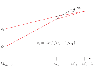
Figure 4: The differences $\delta_{i}=2\pi(1/\alpha_{i}-1/\alpha_{1})$ are plotted as a function of energy scale $\mu$. The threshold correction $\epsilon_{3}$ defined in the 4d GUT scale is used to fix the threshold correction in the 5d orbifold GUT.

4.6 Quarks and Leptons in 5d Orbifold GUTs

Quarks and lepton fields can be put on either of the orbifold “branes” or in the 5d bulk. If they are placed on the $SU(5)$ “brane” at $y=0$, then they come in complete $SU(5)$ multiplets. As a consequence a coupling of the type

$$W\supset\int d^{2}\theta\int dy\ \delta(y)\ \bar{H}\ 10\ \bar{5}$$ (155)

will lead to bottom - tau Yukawa unification. This relation is good for the third generation and so it suggests that the third family should reside on the $SU(5)$ brane. Since this relation does not work for the first two families, they might be placed in the bulk or on the SM brane at $y=\pi\ R$. Without further discussion of quark and lepton masses (see Hall:2002ci ; Kim:2004vk ; Alciati:2005ur ; Alciati:2006sw for complete $SU(5)$ or $SO(10)$ orbifold GUT models), let us consider proton decay in orbifold GUTs.

4.7 Proton Decay

4.7.1 Dimension 6 Operators

The interactions contributing to proton decay are those between the so-called $X$ gauge bosons $A_{\mu}^{(+-)}\in V(+-)$ (where ${A_{\mu}^{(+-)}}^{ai}(x_{\mu},y)$ is the five dimensional gauge boson with quantum numbers $(\bar{3},2,+5/3)$ under SU(3)$\times$ SU(2) $\times$ U(1), $a$ and $i$ are color and SU(2) indices respectively) and the ${\mathcal{N}}=1$ chiral multiplets on the $SU(5)$ brane at $y=0$. Assuming all quarks and leptons reside on this brane we obtain the $\Delta B\neq 0$ interactions given by

$${\cal S}_{\Delta B\neq 0}=-\frac{g_{5}}{\sqrt{2}}\int d^{4}x{A_{\mu}^{(+-)}}^{ai}(x_{\mu},0)J_{ai}^{\mu}(x_{\mu})+h.c.~{}~{}~{}.$$ (156)

The currents $J_{ai}^{\mu}$ are given by:

$$J_{ai}^{\mu} = \epsilon_{abc}\,\epsilon_{ij}(u^{c})^{*}_{b}\,\bar{\sigma}^{\mu}\,q^{cj}+q_{ai}^{*}\,\bar{\sigma}^{\mu}\,e^{c}-\tilde{l}_{i}^{*}\,\bar{\sigma}^{\mu}\,(d^{c})_{a}$$ (157)

$$= (u^{c})^{*}\,\bar{\sigma}^{\mu}\,q+q^{*}\,\bar{\sigma}^{\mu}\,e^{c}-\tilde{l}^{*}\,\bar{\sigma}^{\mu}\,d^{c}~{}~{}~{},$$

Upon integrating out the $X$ gauge bosons we obtain the effective lagrangian for proton decay

$${\cal L}=-\frac{g_{G}^{2}}{2M_{X}^{2}}\sum_{i,j}\left[({q^{*}_{i}}\bar{\sigma}^{\mu}u^{c}_{i})\;(\tilde{l}^{*}_{j}\bar{\sigma}_{\mu}d^{c}_{j})\ +\ (q^{*}_{i}\bar{\sigma}^{\mu}e^{c}_{i})\;(q^{*}_{j}\bar{\sigma}_{\mu}u^{c}_{j})\right]~{}~{}~{},$$ (158)

where all fermions are weak interaction eigenstates and $i,j,k=1,2,3$ are family indices. The dimensionless quantity

$$g_{G}\equiv g_{5}\frac{1}{\sqrt{2\pi R}}$$ (159)

is the four-dimensional gauge coupling of the gauge bosons zero modes. The combination

$$M_{X}=\frac{M_{c}}{\pi}~{}~{}~{},$$ (160)

proportional to the compactification scale

$$M_{c}\equiv\frac{1}{R}~{}~{}~{},$$ (161)

is an effective gauge vector boson mass arising from the sum over all the Kaluza-Klein levels:

$$\sum_{n=0}^{\infty}\frac{4}{(2n+1)^{2}M_{c}^{2}}=\frac{1}{M_{X}^{2}}~{}~{}~{}.$$ (162)

Before one can evaluate the proton decay rate one must first rotate the quark and lepton fields to a mass eigenstate basis. This will bring in both left- and right-handed quark and lepton mixing angles. However, since the compactification scale is typically lower than the 4d GUT scale, it is clear that proton decay via dimension 6 operators is likely to be enhanced.

4.7.2 Dimension 5 Operators

The dimension 5 operators for proton decay result from integrating out color triplet Higgs fermions. However in this simplest $SU(5)$ 5d model the color triplet mass is of the form ArkaniHamed:2001tb

$$W\supset\int d^{2}\theta\ dy\ (T(-+)^{c}\ \partial_{y}\ T(+-)+\bar{T}(-+)^{c}\ \partial_{y}\ \bar{T}(+-))$$ (163)

where a sum over massive KK modes is understood. Since only $T,\ \bar{T}$ couple directly to quarks and leptons, no dimension 5 operators are obtained when integrating out the color triplet Higgs fermions.

4.7.3 Dimension 4 baryon and lepton violating operators

If the theory is constructed with an R parity or family reflection symmetry, then no such operators will be generated.

5 Heterotic String Orbifolds and Orbifold GUTs

6 Phenomenological guidelines

We use the following guidelines when searching for “realistic” string models Lebedev:2006kn ; Lebedev:2007hv . We want to:

1. Preserve gauge coupling unification;

2. Low energy SUSY as solution to the gauge hierarchy problem, i.e. why is $M_{Z}<<M_{G}$;

3. Put quarks and leptons in 16 of SO(10);

4. Put Higgs in 10, thus quarks and leptons are distinguished from Higgs by their SO(10) quantum numbers;

5. Preserve GUT relations for 3rd family Yukawa couplings;

6. Use the fact that GUTs accommodate a “Natural” See-Saw scale ${\cal O}(M_{G})$;

7. Use intuition derived from Orbifold GUT constructions, Kobayashi:2004ud ; Kobayashi:2004ya and

8. Use local GUTs to enforce family structure Forste:2004ie ; Buchmuller:2005jr ; Buchmuller:2006ik .

It is the last two guidelines which are novel and characterize our approach. As a final comment, the string theory analysis discussed here assumes supersymmetric vacua at the string scale. As a consequence there are generically a multitude of moduli. The gauge and Yukawa couplings depend on the values of the moduli vacuum expectation values [VEVs]. In addition vector-like exotics can have mass proportional to the moduli VEVs. We will assume arbitrary values for these moduli VEVs along supersymmetric directions, in order to obtain desirable low energy phenomenology. Of course, at some point supersymmetry must be broken and these moduli must be stabilized. We save this harder problem for a later date. Nevertheless, we can add one more guideline at this point. In the supersymmetric limit, we want the superpotential to have a vanishing VEV. This is so that we can work in flat Minkowski space when considering supergravity. Some of our models naturally have this property.

6.1 $E_{8}\times E_{8}$ 10D heterotic string compactified on $\mathbb{Z}_{3}\times\mathbb{Z}_{2}$ 6D orbifold

There are many reviews and books on string theory. I cannot go into great detail here, so I will confine my discussion to some basic points. We start with the 10d heterotic string theory, consisting of a 26d left-moving bosonic string and a 10d right-moving superstring. Modular invariance requires the momenta of the internal left-moving bosonic degrees of freedom (16 of them) to lie in a 16d Euclidean even self-dual lattice, we choose to be the ${\rm{E}_{8}}\times{\rm{E}_{8}}$ root lattice.

6.1.1 Heterotic string compactified on $T^{6}/\mathbb{Z}_{6}$

We first compactify the theory on 6d torus defined by the space group action of translations on a factorizable Lie algebra lattice $G_{2}\oplus SU(3)\oplus SO(4)$ (see Fig. 5). Then we mod out by the $\mathbb{Z}_{6}$ action on the three complex compactified coordinates given by $Z^{i}\rightarrow e^{2\pi i{\bf r}_{i}\cdot{\bf v}_{6}}Z^{i}$, $i=1,2,3$, where ${\bf v}_{6}=\frac{1}{6}(1,2,-3)$ is the twist vector, and ${\bf r}_{1}=(1,0,0,0)$, ${\bf r}_{2}=(0,1,0,0)$, ${\bf r}_{3}=(0,0,1,0)$. For simplicity and definiteness, we also take the compactified space to be a factorizable Lie algebra lattice $G_{2}\oplus SU(3)\oplus SO(4)$ (see Fig. 5).

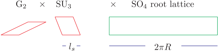
Figure 5: $G_{2}\oplus SU(3)\oplus SO(4)$ lattice. Note, we have taken 5 directions with string scale length $\ell_{s}$ and one with length $2\pi R\gg\ell_{s}$. This will enable the analogy of an effective 5d orbifold field theory.

The $\mathbb{Z}_{6}$ orbifold is equivalent to a $\mathbb{Z}_{2}\times\mathbb{Z}_{3}$ orbifold, where the two twist vectors are ${\bf v}_{2}=3{\bf v}_{6}=\frac{1}{2}(1,0,-1)$ and ${\bf v}_{3}=2{\bf v}_{6}=\frac{1}{3}(1,-1,0)$. The $\mathbb{Z}_{2}$ and $\mathbb{Z}_{3}$ sub-orbifold twists have the $SU(3)$ and $SO(4)$ planes as their fixed torii. In Abelian symmetric orbifolds, gauge embeddings of the point group elements and lattice translations are realized by shifts of the momentum vectors, ${\bf P}$, in the $E_{8}\times E_{8}$ root lattice IMNQ , i.e., ${\bf P}\rightarrow{\bf P}+k{\bf V}+l{\bf W}$, where $k,l$ are some integers, and ${\bf V}$ and ${\bf W}$ are known as the gauge twists and Wilson lines wl . These embeddings are subject to modular invariance requirements Dixon ; vafa . The Wilson lines are also required to be consistent with the action of the point group. In the $\mathbb{Z}_{6}$ model, there are at most three consistent Wilson lines kobayashi , one of degree 3 (${\bf W}_{3}$), along the $SU(3)$ lattice, and two of degree 2 (${\bf W}_{2},\,{\bf W}_{2}^{\prime}$), along the $SO(4)$ lattice.

The $\mathbb{Z}_{6}$ model has three untwisted sectors ($U_{i},\,i=1,2,3$) and five twisted sectors ($T_{i},\,i=1,2,\cdots,5$). (The $T_{k}$ and $T_{6-k}$ sectors are CPT conjugates of each other.) The twisted sectors split further into sub-sectors when discrete Wilson lines are present. In the $SU(3)$ and $SO(4)$ directions, we can label these sub-sectors by their winding numbers, $n_{3}=0,1,2$ and $n_{2},\,n^{\prime}_{2}=0,1$, respectively. In the $G_{2}$ direction, where both the $\mathbb{Z}_{2}$ and $\mathbb{Z}_{3}$ sub-orbifold twists act, the situation is more complicated. There are four $\mathbb{Z}_{2}$ fixed points in the $G_{2}$ plane. Not all of them are invariant under the $\mathbb{Z}_{3}$ twist, in fact three of them are transformed into each other. Thus for the $T_{3}$ twisted-sector states one needs to find linear combinations of these fixed-point states such that they have definite eigenvalues, $\gamma=1$ (with multiplicity 2), $e^{i2\pi/3}$, or $e^{i4\pi/3}$, under the orbifold twist DFMS ; kobayashi (see Fig. 6). Similarly, for the $T_{2,4}$ twisted-sector states, $\gamma=1$ (with multiplicity 2) and $-1$ (the fixed points of the $T_{2,4}$ twisted sectors in the $G_{2}$ torus are shown in Fig. 7). The $T_{1}$ twisted-sector states have only one fixed point in the $G_{2}$ plane, thus $\gamma=1$ (see Fig. 8). The eigenvalues $\gamma$ provide another piece of information to differentiate twisted sub-sectors.

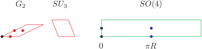
Figure 6: $G_{2}\oplus SU(3)\oplus SO(4)$ lattice with $\mathbb{Z}_{2}$ fixed points. The $T_{3}$ twisted sector states sit at these fixed points. The fixed point at the origin and the symmetric linear combination of the red (grey) fixed points in the $G_{2}$ torus have $\gamma=1$.

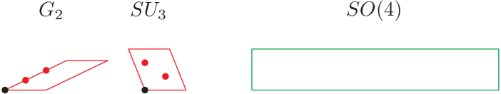
Figure 7: $G_{2}\oplus SU(3)\oplus SO(4)$ lattice with $\mathbb{Z}_{3}$ fixed points for the $T_{2}$ twisted sector. The fixed point at the origin and the symmetric linear combination of the red (grey) fixed points in the $G_{2}$ torus have $\gamma=1$.

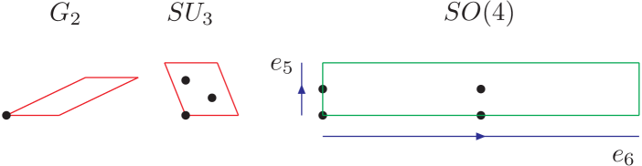
Figure 8: $G_{2}\oplus SU(3)\oplus SO(4)$ lattice with $\mathbb{Z}_{6}$ fixed points. The $T_{1}$ twisted sector states sit at these fixed points.

Massless states in 4d string models consist of those momentum vectors ${\bf P}$ and ${\bf r}$ ($\bf r$ are in the $SO(8)$ weight lattice) which satisfy the following mass-shell equations Dixon ; IMNQ ,

$$\frac{\alpha^{\prime}}{2}m_{R}^{2}=N^{k}_{R}+\frac{1}{2}\left|{\bf r}+k{\bf v}\right|^{2}+a^{k}_{R}=0\,,$$ (164)

$$\frac{\alpha^{\prime}}{2}m_{L}^{2}=N_{L}^{k}+\frac{1}{2}\left|{\bf P}+k{\bf X}\right|^{2}+a_{L}^{k}=0\,,$$ (165)

where $\alpha^{\prime}$ is the Regge slope, $N^{k}_{R}$ and $N^{k}_{L}$ are (fractional) numbers of the right- and left-moving (bosonic) oscillators, ${\bf X}={\bf V}+n_{3}{\bf W}_{3}+n_{2}{\bf W}_{2}+n_{2}^{\prime}{\bf W}_{2}^{\prime}$, and $a^{k}_{R}$, $a_{L}^{k}$ are the normal ordering constants,

$$a^{k}_{R} = -\frac{1}{2}+\frac{1}{2}\sum_{i=1}^{3}|{\widehat{kv_{i}}}|\left(1-|{\widehat{kv_{i}}}|\right)\,,$$

$$a_{L}^{k} = -1+\frac{1}{2}\sum_{i=1}^{3}|{\widehat{kv_{i}}}|\left(1-|{\widehat{kv_{i}}}|\right)\,,$$ (166)

with $\widehat{kv_{i}}={\rm mod}(kv_{i},1)$.

These states are subject to a generalized Gliozzi-Scherk-Olive (GSO) projection ${\cal P}=\frac{1}{6}\sum_{\ell=0}^{5}\Delta^{\ell}$ IMNQ . For the simple case of the $k$-th twisted sector ($k=0$ for the untwisted sectors) with no Wilson lines ($n_{3}=n_{2}=n^{\prime}_{2}=0$) we have

$$\Delta=\gamma\phi\exp\left\{i\pi\biggl{[}(2{\bf P}+k{\bf X})\cdot{\bf X}-(2{\bf r}+k{\bf v})\cdot{\bf v}\biggr{]}\right\},$$ (167)

where $\phi$ are phases from bosonic oscillators. However, in the $\mathbb{Z}_{6}$ model, the GSO projector must be modified for the untwisted-sector and $T_{2,4}$, $T_{3}$ twisted-sector states in the presence of Wilson lines Kobayashi:2004ya . The Wilson lines split each twisted sector into sub-sectors and there must be additional projections with respect to these sub-sectors. This modification in the projector gives the following projection conditions,

$${\bf P}\cdot{\bf V}-{\bf r}_{i}\cdot{\bf v}=\mathbb{Z}\,\,\,\,(i=1,2,3),\quad{\bf P}\cdot{\bf W}_{3},\,\,{\bf P}\cdot{\bf W}_{2},\,\,{\bf P}\cdot{\bf W}_{2}^{\prime}=\mathbb{Z},$$ (168)

for the untwisted-sector states, and

$$T_{2,4}:\,{\bf P}\cdot{\bf W}_{2},\,\,{\bf P}\cdot{\bf W}_{2}^{\prime}={\mathbb{Z}}\,,\qquad T_{3}:\,{\bf P}\cdot{\bf W}_{3}={\mathbb{Z}}\,,$$ (169)

for the $T_{2,3,4}$ sector states (since twists of these sectors have fixed torii). There is no additional condition for the $T_{1}$ sector states.

6.1.2 An orbifold GUT – heterotic string dictionary

We first implement the $\mathbb{Z}_{3}$ sub-orbifold twist, which acts only on the $G_{2}$ and $SU(3)$ lattices. The resulting model is a 6d gauge theory with ${\cal N}=2$ hypermultiplet matter, from the untwisted and $T_{2,4}$ twisted sectors. This 6d theory is our starting point to reproduce the orbifold GUT models. The next step is to implement the $\mathbb{Z}_{2}$ sub-orbifold twist. The geometry of the extra dimensions closely resembles that of 6d orbifold GUTs. The $SO(4)$ lattice has four $\mathbb{Z}_{2}$ fixed points at $0$, $\pi R$, $\pi R^{\prime}$ and $\pi(R+R^{\prime})$, where $R$ and $R^{\prime}$ are on the $e_{5}$ and $e_{6}$ axes, respectively, of the lattice (see Figs. 6 and 8). When one varies the modulus parameter of the $SO(4)$ lattice such that the length of one axis ($R$) is much larger than the other ($R^{\prime}$) and the string length scale ($\ell_{s}$), the lattice effectively becomes the $S^{1}/\mathbb{Z}_{2}$ orbi-circle in the 5d orbifold GUT, and the two fixed points at $0$ and $\pi R$ have degree-2 degeneracies. Furthermore, one may identify the states in the intermediate $\mathbb{Z}_{3}$ model, i.e. those of the untwisted and $T_{2,4}$ twisted sectors, as bulk states in the orbifold GUT.

Space-time supersymmetry and GUT breaking in string models work exactly as in the orbifold GUT models. First consider supersymmetry breaking. In the field theory, there are two gravitini in 4d, coming from the 5d (or 6d) gravitino. Only one linear combination is consistent with the space reversal, $y\rightarrow-y$; this breaks the ${\cal N}=2$ supersymmetry to that of ${\cal N}=1$. In string theory, the space-time supersymmetry currents are represented by those half-integral $SO(8)$ momenta. The $\mathbb{Z}_{3}$ and $\mathbb{Z}_{2}$ projections remove all but two of them, ${\bf r}=\pm\frac{1}{2}(1,1,1,1)$; this gives ${\cal N}=1$ supersymmetry in 4d.

Now consider GUT symmetry breaking. As usual, the $\mathbb{Z}_{2}$ orbifold twist and the translational symmetry of the $SO(4)$ lattice are realized in the gauge degrees of freedom by degree-2 gauge twists and Wilson lines respectively. To mimic the 5d orbifold GUT example, we impose only one degree-2 Wilson line, ${\bf W}_{2}$, along the long direction of the $SO(4)$ lattice, ${\bf R}$. The gauge embeddings generally break the 5d/6d (bulk) gauge group further down to its subgroups, and the symmetry breaking works exactly as in the orbifold GUT models. This can clearly be seen from the following string theoretical realizations of the orbifold parities

$$P=p\,e^{2\pi i\,[{\bf P}\cdot{\bf V}_{2}-{\bf r}\cdot{\bf v}_{2}]}\,,\quad P^{\prime}=p\,e^{2\pi i\,[{\bf P}\cdot({\bf V}_{2}+{\bf W}_{2})-{\bf r}\cdot{\bf v}_{2}]}\,,$$ (170)

where ${\bf V}_{2}=3{\bf V}_{6}$, and $p=\gamma\phi$ can be identified with intrinsic parities in the field theory language. Since $2({\bf P}\cdot{\bf V}_{2}-{\bf r}\cdot{\bf v}_{2}),\,2{\bf P}\cdot{\bf W}_{2}=\mathbb{Z}$, by properties of the $E_{8}\times E_{8}$ and $SO(8)$ lattices, thus $P^{2}=P^{\prime 2}=1$, and Eq. (170) provides a representation of the orbifold parities. From the string theory point of view, $P=P^{\prime}=+$ are nothing but the projection conditions, $\Delta=1$, for the untwisted and $T_{2,4}$ twisted-sector states (see Eqs. (167), (168) and (169)).

To reaffirm this identification, we compare the masses of KK excitations derived from string theory with that of orbifold GUTs. The coordinates of the $SO(4)$ lattice are untwisted under the $\mathbb{Z}_{3}$ action, so their mode expansions are the same as that of toroidal coordinates. Concentrating on the ${\bf R}$ direction, the bosonic coordinate is $X_{L,R}=x_{L,R}+p_{L,R}(\tau\pm\sigma)+{\rm oscillator\,terms}$, with $p_{L}$, $p_{R}$ given by

$$p_{L}= \frac{m}{2R}+\left(1-\frac{1}{4}|{\bf W}_{2}|^{2}\right)\frac{n_{2}R}{\ell_{s}^{2}}+\frac{{\bf P}\cdot{\bf W}_{2}}{2R}\,,\qquad$$

$$p_{R}= p_{L}-\frac{2n_{2}R}{\ell_{s}^{2}}\,,$$ (171)

where $m$ ($n_{2}$) are KK levels (winding numbers). The ${\mathbb{Z}}_{2}$ action maps $m$ to $-m$, $n_{2}$ to $-n_{2}$ and ${\bf W}_{2}$ to $-{\bf W}_{2}$, so physical states must contain linear combinations, $|m,n_{2}\rangle\pm|-m,-n_{2}\rangle$; the eigenvalues $\pm 1$ correspond to the first ${\mathbb{Z}}_{2}$ parity, $P$, of orbifold GUT models. The second orbifold parity, $P^{\prime}$, induces a non-trivial degree-2 Wilson line; it shifts the KK level by $m\rightarrow m+{\bf P}\cdot{\bf W}_{2}$. Since $2{\bf W}_{2}$ is a vector of the (integral) $E_{8}\times E_{8}$ lattice, the shift must be an integer or half-integer. When $R\gg R^{\prime}\sim\ell_{s}$, the winding modes and the KK modes in the smaller dimension of $SO(4)$ decouple. Eq. (171) then gives four types of KK excitations, reproducing the field theoretical mass formula in Eq. (136).

6.2 MSSM with R parity

In this section we discuss just one “benchmark” model (Model 1) obtained via a “mini-landscape” search Lebedev:2006kn of the $E_{8}\times E_{8}$ heterotic string compactified on the $\mathbb{Z}_{6}$ orbifold Lebedev:2007hv . The model is defined by the shifts and Wilson lines

$$V = \left(\frac{1}{3},-\frac{1}{2},-\frac{1}{2},0,0,0,0,0\right)\,\left(\frac{1}{2},-\frac{1}{6},-\frac{1}{2},-\frac{1}{2},-\frac{1}{2},-\frac{1}{2},-\frac{1}{2},\frac{1}{2}\right)\;,$$

$$W_{2} = \left(0,-\frac{1}{2},-\frac{1}{2},-\frac{1}{2},\frac{1}{2},0,0,0\right)\,\left(4,-3,-\frac{7}{2},-4,-3,-\frac{7}{2},-\frac{9}{2},\frac{7}{2}\right)\;,$$

$$W_{3} = \left(-\frac{1}{2},-\frac{1}{2},\frac{1}{6},\frac{1}{6},\frac{1}{6},\frac{1}{6},\frac{1}{6},\frac{1}{6}\right)\,\left(\frac{1}{3},0,0,\frac{2}{3},0,\frac{5}{3},-2,0\right)\;.$$ (172a)

A possible second order 2 Wilson line is set to zero.

The shift $V$ is defined to satisfy two criteria.

• The first criterion is the existence of a local $SO(10)$ GUT at the $T_{1}$ fixed points at $x_{6}=0$ in the $SO(4)$ torus (Fig. 8).

  $$P\cdot V=\mathbb{Z};\;P\in SO(10)\;\;{\rm momentum\;lattice}.$$ (173)

  Since the $T_{1}$ twisted sector has no invariant torus and only one Wilson line along the $x_{6}$ direction, all states located at these two fixed points must come in complete $SO(10)$ multiplets.

• The second criterion is that two massless spinor representations of $SO(10)$ are located at the $x_{6}=0$ fixed points.

Hence, the two complete families on the local $SO(10)$ GUT fixed points gives us an excellent starting point to find the MSSM. The Higgs doublets and third family of quarks and leptons must then come from elsewhere.

Let us now discuss the effective 5d orbifold GUT Dundee:2008ts . Consider the orbifold $(T^{2})^{3}/\mathbb{Z}_{3}$ plus the Wilson line $W_{3}$ in the $SU_{3}$ torus. The $\mathbb{Z}_{3}$ twist does not act on the $SO_{4}$ torus, see Fig. 7. As a consequence of embedding the $\mathbb{Z}_{3}$ twist as a shift in the $E_{8}\times E_{8}$ group lattice and taking into account the $W_{3}$ Wilson line, the first $E_{8}$ is broken to $SU(6)$. This gives the effective 5d orbifold gauge multiplet contained in the ${\mathcal{N}}=1$ vector field $V$. In addition we find the massless states $\Sigma\in{\bf 35}$, ${\bf 20}+{\bf 20}^{c}$ and 18 (${\bf 6}+{\bf 6}^{c}$) in the 6d untwisted sector and $T_{2},\ T_{4}$ twisted sectors. Together these form a complete ${\mathcal{N}}=2$ gauge multiplet ($V+\Sigma$) and a 20 + 18 (6) dimensional hypermultiplets. In fact the massless states in this sector can all be viewed as “bulk” states moving around in a large 5d space-time.

Now consider the $\mathbb{Z}_{2}$ twist and the Wilson line $W_{2}$ along the $x_{6}$ axis in the $SO_{4}$ torus. The action of the $\mathbb{Z}_{2}$ twist breaks the gauge group to $SU(5)$, while $W_{2}$ breaks $SU(5)$ further to the SM gauge group $SU(3)_{C}\times SU(2)_{L}\times U(1)_{Y}$.

Let us now consider those MSSM states located in the bulk. From two of the pairs of ${\mathcal{N}}=1$ chiral multiplets $\bf{6}+\bf{6}^{c}$, which decompose as

$$2\times(\bf 6+\bf 6^{c})\supset$$ (174)

$$\left[(1,\bf 2)_{1,1}^{--}+(\bf 3,1)_{-2/3,1/3}^{-+}\right]$$

$$+\left[(1,\bf 2)_{-1,-1}^{++}+(\overline{\bf 3},1)_{2/3,-1/3}^{--}\right]$$

$$+\left[(1,\bf 2)_{1,1}^{-+}+(\bf 3,1)_{-2/3,1/3}^{--}\right]$$

$$+\left[(1,\bf 2)_{-1,-1}^{+-}+(\overline{\bf 3},1)_{2/3,-1/3}^{++}\right],$$

we obtain the third family $b^{c}$ and lepton doublet, $l$. The rest of the third family comes from the $\mathbf{10}+\mathbf{10}^{c}$ of $SU(5)$ contained in the $\mathbf{20}+\mathbf{20}^{c}$ of $SU(6)$, in the untwisted sector.

Now consider the Higgs bosons. The bulk gauge symmetry is $SU(6)$. Under $SU(5)\times U(1)$, the adjoint decomposes as

$$\mathbf{35}\rightarrow\mathbf{24}_{0}+\mathbf{5}_{+1}+\mathbf{5}^{c}_{-1}+1_{0}.$$ (175)

Thus the MSSM Higgs sector emerges from the breaking of the $SU(6)$ adjoint by the orbifold and the model satisfies the property of “gauge-Higgs unification.”

In the models with gauge-Higgs unification, the Higgs multiplets come from the 5d vector multiplet ($V,\Sigma$), both in the adjoint representation of $SU(6)$. $V$ is the 4d gauge multiplet and the 4d chiral multiplet $\Sigma$ contains the Higgs doublets. These states transform as follows under the orbifold parities $(P\,\,P^{\prime})$:

$$V:\>\left(\begin{array}[]{ccc|cc|c}(++)&(++)&(++)&(+-)&(+-)&(-+)\\ (++)&(++)&(++)&(+-)&(+-)&(-+)\\ (++)&(++)&(++)&(+-)&(+-)&(-+)\\ \hline\cr(+-)&(+-)&(+-)&(++)&(++)&(--)\\ (+-)&(+-)&(+-)&(++)&(++)&(--)\\ \hline\cr(-+)&(-+)&(-+)&(--)&(--)&(++)\end{array}\right)$$ (176)

$$\Phi:\>\left(\begin{array}[]{ccc|cc|c}(--)&(--)&(--)&(-+)&(-+)&(+-)\\ (--)&(--)&(--)&(-+)&(-+)&(+-)\\ (--)&(--)&(--)&(-+)&(-+)&(+-)\\ \hline\cr(-+)&(-+)&(-+)&(--)&(--)&(++)\\ (-+)&(-+)&(-+)&(--)&(--)&(++)\\ \hline\cr(+-)&(+-)&(+-)&(++)&(++)&(--)\end{array}\right).$$ (177)

Hence, we have obtained doublet-triplet splitting via orbifolding.

6.3 $D_{4}$ Family Symmetry

Consider the $\mathbb{Z}_{2}$ fixed points. We have four fixed points, separated into an $SU(5)$ and SM invariant pair by the $W_{2}$ Wilson line (see Fig. 9). We find two complete families, one on each of the $SO_{10}$ fixed points and a small set of vector-like exotics (with fractional electric charge) on the other fixed points. Since $W_{2}$ is in the direction orthogonal to the two families, we find a non-trivial $D_{4}$ family symmetry. This will affect a possible hierarchy of fermion masses. We will discuss the family symmetry and the exotics in more detail next.

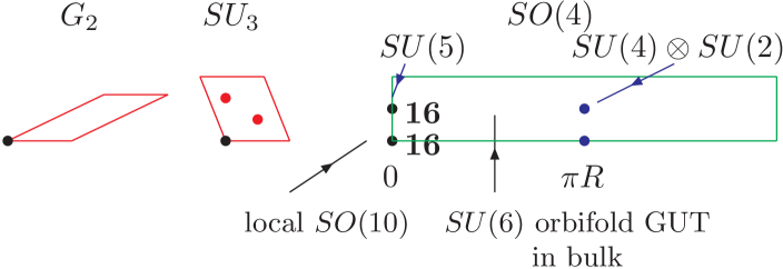
Figure 9: The two families in the $T_{1}$ twisted sector.

The discrete group $D_{4}$ is a non-abelian discrete subgroup of $SU_{2}$ of order 8. It is generated by the set of $2\times 2$ Pauli matrices

$$D_{4}=\{\pm 1,\pm\sigma_{1},\pm\sigma_{3},\mp i\sigma_{2}\}.$$ (178)

In our case, the action of the transformation $\sigma_{1}=\left(\begin{array}[]{cc}0&1\\ 1&0\end{array}\right)$ takes $F_{1}\leftrightarrow F_{2}$, while the action of $\sigma_{3}=\left(\begin{array}[]{cc}1&0\\ 0&-1\end{array}\right)$ takes $F_{2}\rightarrow-F_{2}$. These are symmetries of the string. The first is an unbroken part of the translation group in the direction orthogonal to $W_{2}$ in the $SO_{4}$ torus and the latter is a stringy selection rule resulting from $\mathbb{Z}_{2}$ space group invariance. Under $D_{4}$ the three families of quarks and leptons transform as a doublet, ($F_{1},\ F_{2}$), and a singlet, $F_{3}$. Only the third family can have a tree level Yukawa coupling to the Higgs (which is also a $D_{4}$ singlet). In summary:

• Since the top quarks and the Higgs are derived from the $SU(6)$ chiral adjoint and 20 hypermultiplet in the 5D bulk, they have a tree level Yukawa interaction given by

  $$W\supset\frac{g_{5}}{\sqrt{\pi R}}\int_{0}^{\pi R}dy{\bf{20^{c}}}\ \Sigma\ {\bf 20}=g_{G}\ Q_{3}\ H_{u}\ U^{c}_{3}$$ (179)

  where $g_{5}$ ($g_{G}$) is the 5d (4d) $SU(6)$ gauge coupling constant evaluated at the string scale.

• The first two families reside at the $\mathbb{Z}_{2}$ fixed points, resulting in a $D_{4}$ family symmetry. Hence family symmetry breaking may be used to generate a hierarchy of fermion masses.

6.4 More details of “Benchmark” Model 1 Lebedev:2007hv

Let us now consider the spectrum, exotics, R parity, Yukawa couplings, and neutrino masses. In Table 9 we list the states of the model. In addition to the three families of quarks and leptons and one pair of Higgs doublets, we have vector-like exotics (states which can obtain mass without breaking any SM symmetry) and SM singlets. The SM singlets enter the superpotential in several important ways. They can give mass to the vector-like exotics via effective mass terms of the form

$$EE^{c}\tilde{S}^{n}$$ (180)

where $E,E^{c}$ ($\tilde{S}$) represent the vector-like exotics and SM singlets respectively. We have checked that all vector-like exotics obtain mass at supersymmetric points in moduli space with $F=D=0$. The SM singlets also generate effective Yukawa matrices for quarks and leptons, including neutrinos. In addition, the SM singlets give Majorana mass to the 16 right-handed neutrinos $n^{c}_{i}$, 13 conjugate neutrinos $n_{i}$ and Dirac mass mixing the two. We have checked that the theory has only 3 light left-handed neutrinos.

However, one of the most important constraints in this construction is the existence of an exact low energy R parity. In this model we identified a generalized $B\!-\!L$ (see Table 9) which is standard for the SM states and vector-like on the vector-like exotics. This $B\!-\!L$ naturally distinguishes the Higgs and lepton doublets. Moreover we found SM singlet states

$$\tilde{S}=\{h_{i},\ \chi_{i},\ s_{i}^{0}\}$$ (181)

which can get vacuum expectation values preserving a matter parity $\mathbb{Z}^{\cal M}_{2}$ subgroup of $U(1)_{B\!-\!L}$. It is this set of SM singlets which give vector-like exotics mass and effective Yukawa matrices for quarks and leptons. In addition, the states $\chi_{i}$ give Majorana mass to neutrinos.

As a final note, we have evaluated the $\mu$ term in this model. As a consequence of gauge-Higgs unification, the product $H_{u}H_{d}$ is a singlet under all $U(1)$s. Moreover, it is also invariant under all string selection rules, i.e. H-momentum and space-group selection constraints. As a result the $\mu$ term is of the form

$$\mu\ H_{u}\ H_{d}=W_{0}(\tilde{S})\ H_{u}\ H_{d}$$ (182)

where the factor $W_{0}(\tilde{S})(=\mu)$ is a polynomial in SM singlets and includes all terms which can also appear in the superpotential for the SM singlet fields, $\widetilde{W}_{0}(\tilde{S})$. Thus when we demand a flat space supersymmetric limit, we are also forced to $\mu\equiv W_{0}(\tilde{S})=\widetilde{W}_{0}{\tilde{S}}=0$, i.e. $\mu$ vanishes in the flat space supersymmetric limit. This is encouraging, since when SUSY is broken we expect both terms to be non-vanishing and of order the weak scale.

# irrep label # irrep label 3 $\left(\boldsymbol{3},\boldsymbol{2};\boldsymbol{1},\boldsymbol{1}\right)_{(1/3,1/3)}$ $q_{i}$ 3 $\left(\overline{\boldsymbol{3}},\boldsymbol{1};\boldsymbol{1},\boldsymbol{1}\right)_{(-4/3,-1/3)}$ $u^{c}_{i}$ 3 $\left(\boldsymbol{1},\boldsymbol{1};\boldsymbol{1},\boldsymbol{1}\right)_{(2,1)}$ $e^{c}_{i}$ 8 $\left(\boldsymbol{1},\boldsymbol{2};\boldsymbol{1},\boldsymbol{1}\right)_{(0,*)}$ $m_{i}$ 4 $\left(\overline{\boldsymbol{3}},\boldsymbol{1};\boldsymbol{1},\boldsymbol{1}\right)_{(2/3,-1/3)}$ $d^{c}_{i}$ 1 $\left(\boldsymbol{3},\boldsymbol{1};\boldsymbol{1},\boldsymbol{1}\right)_{(-2/3,1/3)}$ $d_{i}$ 4 $\left(\boldsymbol{1},\boldsymbol{2};\boldsymbol{1},\boldsymbol{1}\right)_{(-1,-1)}$ $\ell_{i}$ 1 $\left(\boldsymbol{1},\boldsymbol{2};\boldsymbol{1},\boldsymbol{1}\right)_{(1,1)}$ $\ell^{c}_{i}$ 1 $\left(\boldsymbol{1},\boldsymbol{2};\boldsymbol{1},\boldsymbol{1}\right)_{(-1,0)}$ $\phi_{i}$ 1 $\left(\boldsymbol{1},\boldsymbol{2};\boldsymbol{1},\boldsymbol{1}\right)_{(1,0)}$ $\phi^{c}_{i}$ 6 $\left(\overline{\boldsymbol{3}},\boldsymbol{1};\boldsymbol{1},\boldsymbol{1}\right)_{(2/3,2/3)}$ $\delta^{c}_{i}$ 6 $\left(\boldsymbol{3},\boldsymbol{1};\boldsymbol{1},\boldsymbol{1}\right)_{(-2/3,-2/3)}$ $\delta_{i}$ 14 $\left(\boldsymbol{1},\boldsymbol{1};\boldsymbol{1},\boldsymbol{1}\right)_{(1,*)}$ $s^{+}_{i}$ 14 $\left(\boldsymbol{1},\boldsymbol{1};\boldsymbol{1},\boldsymbol{1}\right)_{(-1,*)}$ $s^{-}_{i}$ 16 $\left(\boldsymbol{1},\boldsymbol{1};\boldsymbol{1},\boldsymbol{1}\right)_{(0,1)}$ $n^{c}_{i}$ 13 $\left(\boldsymbol{1},\boldsymbol{1};\boldsymbol{1},\boldsymbol{1}\right)_{(0,-1)}$ $n_{i}$ 5 $\left(\boldsymbol{1},\boldsymbol{1};\boldsymbol{1},\boldsymbol{2}\right)_{(0,1)}$ $\eta^{c}_{i}$ 5 $\left(\boldsymbol{1},\boldsymbol{1};\boldsymbol{1},\boldsymbol{2}\right)_{(0,-1)}$ $\eta_{i}$ 10 $\left(\boldsymbol{1},\boldsymbol{1};\boldsymbol{1},\boldsymbol{2}\right)_{(0,0)}$ $h_{i}$ 2 $\left(\boldsymbol{1},\boldsymbol{2};\boldsymbol{1},\boldsymbol{2}\right)_{(0,0)}$ $y_{i}$ 6 $\left(\boldsymbol{1},\boldsymbol{1};\boldsymbol{4},\boldsymbol{1}\right)_{(0,*)}$ $f_{i}$ 6 $\left(\boldsymbol{1},\boldsymbol{1};\overline{\boldsymbol{4}},\boldsymbol{1}\right)_{(0,*)}$ $f^{c}_{i}$ 2 $\left(\boldsymbol{1},\boldsymbol{1};\boldsymbol{4},\boldsymbol{1}\right)_{(-1,-1)}$ $f_{i}^{-}$ 2 $\left(\boldsymbol{1},\boldsymbol{1};\overline{\boldsymbol{4}},\boldsymbol{1}\right)_{(1,1)}$ ${f^{c}_{i}}^{+}$ 4 $\left(\boldsymbol{1},\boldsymbol{1};\boldsymbol{1},\boldsymbol{1}\right)_{(0,\pm 2)}$ $\chi_{i}$ 32 $\left(\boldsymbol{1},\boldsymbol{1};\boldsymbol{1},\boldsymbol{1}\right)_{(0,0)}$ $s^{0}_{i}$ 2 $\left(\overline{\boldsymbol{3}},\boldsymbol{1};\boldsymbol{1},\boldsymbol{1}\right)_{(-1/3,2/3)}$ $v^{c}_{i}$ 2 $\left(\boldsymbol{3},\boldsymbol{1};\boldsymbol{1},\boldsymbol{1}\right)_{(1/3,-2/3)}$ $v_{i}$

Table 9: Spectrum. The quantum numbers under $\mathrm{SU}(3)\times\mathrm{SU}(2)\times[\mathrm{SU}(4)\times\mathrm{SU}(2)^{\prime}]$ are shown in boldface; hypercharge and $B\!-\!L$  charge appear as subscripts. Note that the states $s_{i}^{\pm}$, $f_{i}$, $\bar{f}_{i}$ and $m_{i}$ have different $B-L$ charges for different $i$, which we do not explicitly list Lebedev:2007hv .

6.5 Gauge Coupling Unification and Proton Decay

We have checked whether the SM gauge couplings unify at the string scale in the class of models similar to Model 1 above Dundee:2008ts . All of the 15 MSSM-like models of Ref. Lebedev:2007hv have 3 families of quarks and leptons and one or more pairs of Higgs doublets. They all admit an $SU(6)$ orbifold GUT with gauge-Higgs unification and the third family in the bulk. They differ, however, in other bulk and brane exotic states. We show that the KK modes of the model, including only those of the third family and the gauge sector, are not consistent with gauge coupling unification at the string scale. Nevertheless, we show that it is possible to obtain unification if one adjusts the spectrum of vector-like exotics below the compactification scale. As an example, see Fig. 10. Note, the compactification scale is less than the 4d GUT scale and some exotics have mass two orders of magnitude less than $M_{c}$, while all others are taken to have mass at $M_{\rm STRING}$. In addition, the value of the GUT coupling at the string scale, $\alpha_{G}(M_{STRING})\equiv\alpha_{string}$, satisfies the weakly coupled heterotic string relation

$$G_{N}=\frac{1}{8}\,\alpha_{string}\,\alpha^{\prime}$$ (183)

or

$$\alpha_{string}^{-1}=\frac{1}{8}\,(\frac{M_{Pl}}{M_{\rm STRING}})^{2}.$$ (184)

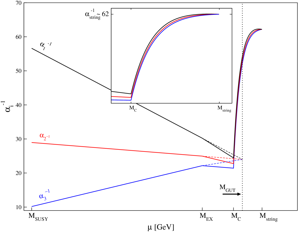
Figure 10: An example of the type of gauge coupling evolution we see in these models, versus the typical behavior in the MSSM. The “tail” is due to the power law running of the couplings when towers of Kaluza-Klein modes are involved. Unification in this model occurs at $M_{\rm STRING}\simeq 5.5\times 10^{17}$ GeV, with a compactification scale of $M_{c}\simeq 8.2\times 10^{15}$ GeV, and an exotic mass scale of $M_{\rm EX}\simeq 8.2\times 10^{13}$ GeV.

In Fig. 11 we plot the distribution of solutions with different choices of light exotics. On the same plot we give the proton lifetime due to dimension 6 operators. Recall in these models the two light families are located on the $SU(5)$ branes, thus the proton decay rate is only suppressed by $M_{c}^{-2}$. Note, 90% of the models are already excluded by the Super-Kamiokande bounds on the proton lifetime. The remaining models may be tested at a next generation megaton water čerenkov detector.

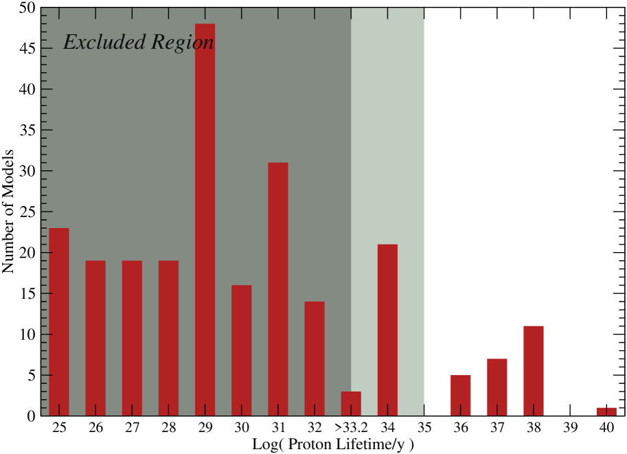
Figure 11: Histogram of solutions with $M_{\rm STRING}>M_{c}\gtrsim M_{\rm EX}$, showing the models which are excluded by Super-K bounds (darker green) and those which are potentially accessible in a next generation proton decay experiment (lighter green). Of 252 total solutions, 48 are not experimentally ruled out by the current experimental bound, and most of the remaining parameter space can be eliminated in the next generation of proposed proton decay searches.

7 Conclusion

In these lectures we have discussed an evolution of SUSY GUT model building. We saw that 4d SUSY GUTs have many virtues. However there are some problems which suggest that these models may be difficult to derive from a more fundamental theory, i.e. string theory. We then discussed orbifold GUT field theories which solve two of the most difficult problems of 4d GUTs, i.e. GUT symmetry breaking and Higgs doublet-triplet splitting. We then showed how some orbifold GUTs can find an ultra-violet completion within the context of heterotic string theory.

The flood gates are now wide open. In recent work Lebedev:2007hv we have obtained many models with features like the MSSM: SM gauge group with 3 families and vector-like exotics which can, in principle, obtain large mass. The models have an exact R-parity and non-trivial Yukawa matrices for quarks and leptons. In addition, neutrinos obtain mass via the See-Saw mechanism. We showed that gauge coupling unification can be accommodated Dundee:2008ts . Recently, another MSSM-like model has been obtained with the heterotic string compactified on a $T^{6}/\mathbb{Z}_{12}$ orbifold Kim:2007mt .

Of course, this is not the end of the story. It is just the beginning. We must still obtain predictions for the LHC. This requires stabilizing the moduli and breaking supersymmetry. In fact, these two conditions are not independent, since once SUSY is broken, the moduli will be stabilized. The scary fact is that the moduli have to be stabilized at just the right values to be consistent with low energy phenomenology.

References

- (1) J. Pati and A. Salam, Phys. Rev. D8 1240 (1973). For more discussion on the standard charge assignments in this formalism, see A. Davidson, Phys. Rev.D20, 776 (1979) and R.N. Mohapatra and R.E. Marshak, Phys. Lett.B91, 222 (1980).
- (2) H. Georgi, Particles and Fields, Proceedings of the APS Div. of Particles and Fields, ed C. Carlson, p. 575 (1975); H. Fritzsch and P. Minkowski, Ann. Phys. 93, 193 (1975).
- (3) H. Georgi and S.L. Glashow, Phys. Rev. Lett. 32 438 (1974).
- (4) S. Dimopoulos, S. Raby and F. Wilczek, Phys. Rev. D24, 1681 (1981); S. Dimopoulos and H. Georgi, Nucl. Phys. B193, 150 (1981); L. Ibanez and G.G. Ross, Phys. Lett. 105B, 439 (1981); N. Sakai, Z. Phys. C11, 153 (1981)
- (5) M. B. Einhorn and D. R. T. Jones, Nucl. Phys. B196, 475 (1982); W. J. Marciano and G. Senjanovic, Phys. Rev. D 25, 3092 (1982).
- (6) W.-M.Yao et al. (Particle Data Group), J. Phys. G 33, 1 (2006) and 2007 partial update for the 2008 edition.
- (7) P. Langacker and N. Polonsky, Phys. Rev. D 52, 3081 (1995) [arXiv:hep-ph/9503214].
- (8) M. L. Alciati, F. Feruglio, Y. Lin and A. Varagnolo, JHEP 0503, 054 (2005) [arXiv:hep-ph/0501086].
- (9) M. S. Carena, S. Pokorski and C. E. M. Wagner, Nucl. Phys. B 406, 59 (1993) [arXiv:hep-ph/9303202].
- (10) M. Gell-Mann, P. Ramond and R. Slansky, in Supergravity, ed. P. van Nieuwenhuizen and D.Z. Freedman, North-Holland, Amsterdam, 1979, p. 315.
- (11) S. Weinberg, Phys. Rev. D26, 287 (1982); N. Sakai and T Yanagida, Nucl. Phys. B197, 533 (1982).
- (12) G. Farrar and P. Fayet, Phys. Lett. B76, 575 (1978).
- (13) S. Dimopoulos, S. Raby and F. Wilczek, Phys. Lett. 112B, 133 (1982); J. Ellis, D.V. Nanopoulos and S. Rudaz, Nucl. Phys. B202, 43 (1982).
- (14) L.E. Ibanez and G.G. Ross, Nucl. Phys. B368, 3 (1992).
- (15) For a recent discussion, see C.S. Aulakh, B. Bajc, A. Melfo, A. Rasin and G. Senjanovic, Nucl. Phys. B597, 89 (2001).
- (16) V. Lucas and S. Raby, Phys. Rev. D54, 2261 (1996) [arXiv:hep-ph/9601303]; T. Blazek, M. Carena, S. Raby and C. E. M. Wagner, Phys. Rev. D56, 6919 (1997) [arXiv:hep-ph/9611217].
- (17) G. Altarelli, F. Feruglio and I. Masina, JHEP 0011, 040 (2000) [arXiv:hep-ph/0007254].
- (18) R. Dermíšek, A. Mafi and S. Raby, Phys. Rev. D63, 035001 (2001); K.S. Babu, J.C. Pati and F. Wilczek, Nucl. Phys. B566, 33 (2000).
- (19) S. Dimopoulos and F. Wilczek, “Incomplete Multiplets In Supersymmetric Unified Models,” Preprint NSF-ITP-82-07 (unpublished).
- (20) K. S. Babu and S. M. Barr, Phys. Rev. D 48, 5354 (1993) [arXiv:hep-ph/9306242].
- (21) See talk by M. Shiozawa at SUSY 2008, Seoul, S. Korea.
- (22) See talks by Matthew Earl, NNN workshop, Irvine, February (2000); Y. Totsuka, SUSY2K, CERN, June (2000); Y. Suzuki, International Workshop on Neutrino Oscillations and their Origins, Tokyo, Japan, December (2000) and Baksan School, Baksan Valley, Russia, April (2001), hep-ex/0110005; K. Kobayashi [Super-Kamiokande Collaboration], “Search for nucleon decay from Super-Kamiokande,” Prepared for 27th International Cosmic Ray Conference (ICRC 2001), Hamburg, Germany, 7-15 Aug 2001. For published results see Super-Kamiokande Collaboration: Y. Hayato, M. Earl, et. al, Phys. Rev. Lett. 83, 1529 (1999); K. Kobayashi et al. [Super-Kamiokande Collaboration], [arXiv:hep-ex/0502026].
- (23) T. Goto and T. Nihei, Phys. Rev. D59, 115009 (1999) [arXiv:hep-ph/9808255]; H. Murayama and A. Pierce, Phys. Rev. D65, 055009 (2002) [arXiv:hep-ph/0108104].
- (24) M. Chanowitz, J. Ellis and M.K. Gaillard, Nucl. Phys. B135, 66 (1978). For the corresponding SUSY analysis, see M. Einhorn and D.R.T. Jones, Nucl. Phys. B196, 475 (1982); K. Inoue, A. Kakuto, H. Komatsu and S. Takeshita, Prog. Theor. Phys. 67, 1889 (1982); L. E. Ibanez and C. Lopez, Phys. Lett. B126, 54 (1983); Nucl. Phys. B233, 511 (1984).
- (25) H. Georgi and D.V. Nanopoulos, Nucl. Phys. B159, 16 (1979)
- (26) J. Harvey, P. Ramond and D.B. Reiss, Phys. Lett. 92B, 309 (1980); Nucl. Phys. B199, 223 (1982).
- (27) T. Banks, Nucl. Phys. B303, 172 (1988); M. Olechowski and S. Pokorski, Phys. Lett. B214, 393 (1988); S. Pokorski, Nucl. Phys. B13 (Proc. Supp.), 606 (1990); B. Ananthanarayan, G. Lazarides and Q. Shafi, Phys. Rev. D44, 1613 (1991); Q. Shafi and B. Ananthanarayan, ICTP Summer School lectures (1991); S. Dimopoulos, L.J. Hall and S. Raby, Phys. Rev. Lett. 68, 1984 (1992), Phys. Rev. D45, 4192 (1992); G. Anderson et al., Phys. Rev. D47, 3702 (1993); B. Ananthanarayan, G. Lazarides and Q. Shafi, Phys. Lett. B300, 245 (1993); G. Anderson et al., Phys. Rev. D49, 3660 (1994); B. Ananthanarayan, Q. Shafi and X.M. Wang, Phys. Rev. D50, 5980 (1994).
- (28) G. Lazarides, Q. Shafi and C. Wetterich, Nucl. Phys. B181, 287 (1981); T. E. Clark, T. K. Kuo and N. Nakagawa, Phys. Lett. B115, 26 (1982); K. S. Babu and R. N. Mohapatra, Phys. Rev. Lett. 70, 2845 (1993) [arXiv:hep-ph/9209215].
- (29) B. Bajc, G. Senjanovic and F. Vissani, Phys. Rev. Lett. 90, 051802 (2003) [arXiv:hep-ph/0210207].
- (30) H. S. Goh, R. N. Mohapatra and S. P. Ng, Phys. Lett. B570, 215 (2003) [arXiv:hep-ph/0303055]; H. S. Goh, R. N. Mohapatra and S. P. Ng, Phys. Rev. D68, 115008 (2003) [arXiv:hep-ph/0308197]; B. Dutta, Y. Mimura and R. N. Mohapatra, Phys. Rev. D69, 115014 (2004) [arXiv:hep-ph/0402113]; S. Bertolini and M. Malinsky, [arXiv:hep-ph/0504241]; K. S. Babu and C. Macesanu, [arXiv:hep-ph/0505200].
- (31) LEP Higgs Working Group and ALEPH collaboration and DELPHI collaboration and L3 collaboration and OPAL Collaboration, Preliminary results, [hep-ex/0107030] (2001).
- (32) M. Carena and H. E. Haber, Prog. Part. Nucl. Phys. 50, 63 (2003) [arXiv:hep-ph/0208209].
- (33) L.J. Hall, R. Rattazzi and U. Sarid, Phys. Rev. D50, 7048 (1994); M. Carena, M. Olechowski, S. Pokorski and C.E.M. Wagner, Nucl. Phys. B419, 213 (1994); R. Rattazzi and U. Sarid, Nucl. Phys. B501, 297 (1997).
- (34) T. Blazek, R. Dermisek and S. Raby, Phys. Rev. Lett. 88, 111804 (2002) [arXiv:hep-ph/0107097]; Phys. Rev. D65, 115004 (2002) [arXiv:hep-ph/0201081];
- (35) K. Tobe and J. D. Wells, [arXiv:hep-ph/0301015].
- (36) D. Auto, H. Baer, C. Balazs, A. Belyaev, J. Ferrandis and X. Tata, [arXiv:hep-ph/0302155].
- (37) C. Balazs and R. Dermisek, arXiv:hep-ph/0303161.
- (38) H. Baer, S. Kraml, S. Sekmen and H. Summy, JHEP 0803, 056 (2008) [arXiv:0801.1831 [hep-ph]].
- (39) J. A. Bagger, J. L. Feng, N. Polonsky and R. J. Zhang, Phys. Lett. B 473, 264 (2000) [arXiv:hep-ph/9911255].
- (40) F. Gabbiani, E. Gabrielli, A. Masiero and L. Silvestrini, Nucl. Phys. B 477, 321 (1996) [arXiv:hep-ph/9604387]; T. Besmer, C. Greub, and T. Hurth, Nucl. Phys. B 609, 359 (2001) [arXiv:hep-ph/0105292].
- (41) H. Georgi and C. Jarlskog, Phys. Lett. 86B 297 (1979).
- (42) K.S. Babu and R.N. Mohapatra, Phys. Rev. Lett.74, 2418 (1995); V. Lucas and S. Raby, Phys. Rev. D54, 2261 (1996); T. Blažek, M. Carena, S. Raby and C. Wagner, Phys. Rev. D56, 6919 (1997); R. Barbieri, L.J. Hall, S. Raby and A. Romanino, Nucl. Phys. B493, 3 (1997); T. Blazek, S. Raby and K. Tobe, Phys. Rev. D60, 113001 (1999), Phys. Rev. D62 055001 (2000); Q. Shafi and Z. Tavartkiladze, Phys. Lett. B487, 145 (2000); C.H. Albright and S.M. Barr, Phys. Rev. Lett. 85, 244 (2000); K.S. Babu, J.C. Pati and F. Wilczek, Nucl. Phys. B566, 33 (2000); G. Altarelli, F. Feruglio, I. Masina, Ref. af; Z. Berezhiani and A. Rossi, Nucl. Phys. B594, 113 (2001); C. H. Albright and S. M. Barr, Phys. Rev. D64, 073010 (2001) [arXiv:hep-ph/0104294]; R. Dermisek and S. Raby, Phys. Lett. B622, 327 (2005) [arXiv:hep-ph/0507045].
- (43) S. Weinberg, I.I. Rabi Festschrift (1977); F. Wilczek and A. Zee, Phys. Lett.70B 418 (1977); H. Fritzsch, Phys. Lett.70B 436 (1977).
- (44) H. D. Kim, S. Raby and L. Schradin, Phys. Rev. D 69, 092002 (2004) [arXiv:hep-ph/0401169].
- (45) L. J. Hall and A. Rasin, Phys. Lett. B 315, 164 (1993) [arXiv:hep-ph/9303303].
- (46) P. Minkowski, Phys. Lett.B67, 421 (1977).
- (47) T. Yanagida, in Proceedings of the Workshop on the unified theory and the baryon number of the universe, ed. O. Sawada and A. Sugamoto, KEK report No. 79-18, Tsukuba, Japan, 1979; S. Glashow, Quarks and leptons , published in Proceedings of the Carg‘ese Lectures, M. L evy (ed.), Plenum Press, New York, (1980); M. Gell-Mann, P. Ramond and R. Slansky, in Supergravity, ed. P. van Nieuwenhuizen and D.Z. Freedman, North-Holland, Amsterdam, (1979), p. 315; R.N. Mohapatra and G. Senjanovic, Phys. Rev. Lett. 44, 912 (1980).
- (48) R. Dermisek and S. Raby, Phys. Lett. B 622, 327 (2005) [arXiv:hep-ph/0507045].
- (49) R. Dermisek, M. Harada and S. Raby, Phys. Rev. D 74, 035011 (2006) [arXiv:hep-ph/0606055].
- (50) M. Albrecht, W. Altmannshofer, A. J. Buras, D. Guadagnoli and D. M. Straub, JHEP 0710, 055 (2007) [arXiv:0707.3954 [hep-ph]].
- (51) W. Altmannshofer, D. Guadagnoli, S. Raby and D. M. Straub, arXiv:0801.4363 [hep-ph].
- (52) C.D. Froggatt and H.B. Nielsen, Nucl. Phys.B147 277 (1979).
- (53) R. Dermisek, S. Raby, L. Roszkowski and R. Ruiz De Austri, JHEP 0304, 037 (2003) [arXiv:hep-ph/0304101]. R. Dermisek, S. Raby, L. Roszkowski and R. Ruiz de Austri, JHEP 0509, 029 (2005) [arXiv:hep-ph/0507233].
- (54) S. M. Barr and S. Raby, Phys. Rev. Lett. 79, 4748 (1997) [arXiv:hep-ph/9705366].
- (55) A. Masiero, D. V. Nanopoulos, K. Tamvakis and T. Yanagida, Phys. Lett. B115, 380 (1982); B. Grinstein, Nucl. Phys. B206, 387 (1982).
- (56) R. Dermisek, S. Raby and S. Nandi, Nucl. Phys. B 641, 327 (2002) [arXiv:hep-th/0205122].
- (57) L. J. Hall and Y. Nomura, Phys. Rev. D 64, 055003 (2001) [arXiv:hep-ph/0103125].
- (58) Y. Kawamura, Progr. Theor. Phys.103, 613 (2000); ibid. 105, 999 (2001); G. Altarelli, F. Feruglio, Phys. Lett.B511, 257 (2001); A. Hebecker, J. March-Russell, Nucl. Phys. B613, 3 (2001); T. Asaka, W. Buchm uller, L. Covi, Phys. Lett. B523, 199 (2001); L. J. Hall, Y. Nomura, T. Okui, D. R. Smith, Phys. Rev. D65, 035008 (2002); R. Dermisek and A. Mafi, Phys. Rev. D65, 055002 (2002); H. D. Kim and S. Raby, JHEP 0301, 056 (2003).
- (59) K. R. Dienes, E. Dudas and T. Gherghetta, Nucl. Phys. B 537, 47 (1999) [arXiv:hep-ph/9806292].
- (60) R. Contino, L. Pilo, R. Rattazzi and E. Trincherini, Nucl. Phys. B 622, 227 (2002) [arXiv:hep-ph/0108102].
- (61) D. M. Ghilencea and S. Groot Nibbelink, Nucl. Phys. B 641, 35 (2002) [arXiv:hep-th/0204094].
- (62) L. J. Hall and Y. Nomura, Phys. Rev. D 66, 075004 (2002) [arXiv:hep-ph/0205067].
- (63) H. D. Kim, S. Raby and L. Schradin, JHEP 0505, 036 (2005) [arXiv:hep-ph/0411328].
- (64) M. L. Alciati, F. Feruglio, Y. Lin and A. Varagnolo, JHEP 0611, 039 (2006) [arXiv:hep-ph/0603086].
- (65) N. Arkani-Hamed, T. Gregoire and J. G. Wacker, JHEP 0203, 055 (2002) [arXiv:hep-th/0101233].
- (66) O. Lebedev et al., “A mini-landscape of exact MSSM spectra in heterotic orbifolds,” Phys. Lett. B645, 88 (2007).
- (67) O. Lebedev et al., “The heterotic road to the mssm with parity,” arXiv:0708.2691[hep-th].
- (68) T. Kobayashi, S. Raby and R. J. Zhang, Phys. Lett. B 593, 262 (2004) [arXiv:hep-ph/0403065].
- (69) T. Kobayashi, S. Raby and R. J. Zhang, Nucl. Phys. B 704, 3 (2005) [arXiv:hep-ph/0409098].
- (70) S. Forste, H. P. Nilles, P. K. S. Vaudrevange and A. Wingerter, Phys. Rev. D 70, 106008 (2004) [arXiv:hep-th/0406208].
- (71) W. Buchmuller, K. Hamaguchi, O. Lebedev and M. Ratz, Phys. Rev. Lett. 96, 121602 (2006) [arXiv:hep-ph/0511035].
- (72) W. Buchmuller, K. Hamaguchi, O. Lebedev and M. Ratz, Nucl. Phys. B 785, 149 (2007) [arXiv:hep-th/0606187].
- (73) L. E. Ibáñez, J. E. Kim, H.-P. Nilles and F. Quevedo, Phys. Lett. B 191, 282 (1987); L. E. Ibáñez, J. Mas, H. P. Nilles and F. Quevedo, Nucl. Phys. B 301, 157 (1988); A. Font, L. E. Ibáñez, F. Quevedo and A. Sierra, Nucl. Phys. B 331, 421 (1990); D. Bailin, A. Love and S. Thomas, Phys. Lett. B 194, 385 (1987); Y. Katsuki, Y. Kawamura, T. Kobayashi, N. Ohtsubo, Y. Ono and K. Tanioka, Nucl. Phys. B 341, 611 (1990).
- (74) L. E. Ibáñez, H.-P. Nilles and F. Quevedo, Phys. Lett. B 187, 25 (1987).
- (75) L. J. Dixon, J. A. Harvey, C. Vafa and E. Witten, Nucl. Phys. B 261, 678 (1985); Nucl. Phys. B 274, 285 (1986).
- (76) C. Vafa, Nucl. Phys. B 273, 592 (1986).
- (77) T. Kobayashi and N. Ohtsubo, Phys. Lett. B 257, 56 (1991); Inter. J. Mod. Phys. A 9, 87 (1994).
- (78) L. Dixon, D. Friedan, E. Martinec and S. Shenker, Nucl. Phys. B 282, 13 (1987).
- (79) T. Asaka, W. Buchmüller and L. Covi, Phys. Lett. B 523, 199 (2001); L. J. Hall and Y. Nomura, hep-ph/0207079.
- (80) P. Ko, T. Kobayashi, J. h. Park and S. Raby, Phys. Rev. D 76, 035005 (2007) [Erratum-ibid. D 76, 059901 (2007)] [arXiv:0704.2807 [hep-ph]].
- (81) T. Kobayashi, H. P. Nilles, F. Ploger, S. Raby and M. Ratz, Nucl. Phys. B 768, 135 (2007) [arXiv:hep-ph/0611020].
- (82) B. Dundee, S. Raby and A. Wingerter, arXiv:0805.4186 [hep-th].
- (83) J. E. Kim, J. H. Kim and B. Kyae, JHEP 0706, 034 (2007) [arXiv:hep-ph/0702278]; J. E. Kim and B. Kyae, Phys. Rev. D 77, 106008 (2008) [arXiv:0712.1596 [hep-th]].