High Energy Neutrinos and Photons from Curvature Pions in Magnetars

Abstract

We discuss the relevance of the curvature radiation of pions in strongly magnetized pulsars or magnetars, and their implications for the production of TeV energy neutrinos detectable by cubic kilometer scale detectors, as well as high energy photons.

1 Introduction

In pulsar and magnetar polar caps one expects the formation of vacuum or space-charge limited gaps (e.g. Harding and Lai, 2006), in which an electric field component parallel to the magnetic field accelerates particles to relativistic velocities. The particles move away from the caps along the magnetic field lines, producing photons by curvature radiation, which at some height $h$ produce an $e^{\pm}$ pair front that determines the upper extent of the gap (e.g. Ruderman and Sutherland, 1975, Harding and Muslimov, 2002). The caps with $\Omega\cdot B<0$ can accelerate positively charged protons or ions, whose interaction with X-rays from the polar cap will lead to very high energy (VHE, $E\lower 4.0pt\hbox{$\buildrel>\over{\sim}$}10^{12}$ eV) neutrinos through photomeson interactions, $p\gamma\to\pi^{+}\to\mu^{+}\nu_{\mu}\to e^{+}\nu_{e}{\bar{\nu}}_{\mu}$ (Zhang et al, 2003). Here we explore the consequences for neutrino production of a different mechanism, the curvature radiation of pions by protons.

Relativistic protons interacting with a strong magnetic field can produce pions, a quantum treatment of this process being given by Zharkov (1964). Ginzburg and Zharkov (1965) used a semi-classical approach to emphasize the analogy between this pion radiation process and the usual synchrotron radiation of photons by protons. This semi-classical method was further explored for $\pi^{0}$ and $\rho$ mesons by Tokuhisa and Kajino (1999) in the context of pulsars. The pion radiation mechanism is characterized by a parameter $\chi=\gamma^{2}(B/B_{Q})$ similar to that used for electron processes but with the proton mass replacing the electron mass, with $B_{Q}=m_{p}^{2}c^{3}/e\hbar=1.5\times 10^{20}$ G. They showed that the synchrotron-like $\pi^{0}$ radiation process becomes competitive with (proton) photon synchrotron radiation when the above parameter $\chi\lower 4.0pt\hbox{$\buildrel>\over{\sim}$}0.1$. The related synchrotron-like $\pi^{+}$ radiation by protons in a magnetic field requires, however, a different semi-classical treatment, since the protons become neutrons in the process, and this was calculated by Herpay and Patkós (2008).

In the astrophysical literature, particle acceleration in pulsars or magnetars is considered both near the polar caps (“inner” or polar gap models), and further out near or beyond the light cylinder (“outer” gap or wind models); e.g. see review by Harding and Lai (2006). Examples of the former are e.g. Blasi, Epstein and Olinto (2000), Arons (2003), etc.; while examples of the latter are, e.g. Sutherland (1979), Harding and Muslimov (2001, 2002, 2005), Thompson (2008), etc.. Here, we consider specifically the case of protons or ions accelerated in the inner regions, just above the polar caps of magnetars. In the inner acceleration region discussed here, the accelerated particles are expected to radiate away their transverse energy so efficiently that they are effectively constrained to the ground Landau level as they move along the curved field lines. The principal photon radiation loss is then curvature radiation (Ruderman and Sutherland, 1975; Harding and Lai, 2006). In this situation, the synchrotron-like pion radiation (which depends on the proton transverse energy) will be similarly suppressed. However, as for photon curvature radiation, the motion along the curved field lines produces an acceleration equivalent to a Larmor motion in a fictitious magnetic field, which will lead to curvature pion radiation (Berezinsky, Dolgov and Kachelriess, 1996). Unlike previous authors, in this paper we concentrate on $\pi^{\pm}$ production by the curvature-like mechanism of both protons and heavy nuclei, occurring in the immediate vicinity of the polar caps, and we explore its consequences for the production of VHE neutrinos, as well as their detectability by cubic kilometer Cherenkov detectors such as IceCube and KM3NeT. We compare the resulting neutrino fluxes to those from the photomeson process, and discuss the associated cosmic ray as well as GeV-TeV photon production.

In §2 we discuss an approximate acceleration and radiation loss model, including both photon and pion radiation losses. Simple time-scale arguments are presented to estimate the maximum particle energies possible and the ratio of photon to pion losses. In §3 we consider in more detail the equations of motion in self-consistent polar cap magnetic field models, and calculate numerically the acceleration and energy loss rates in a general manner. These results are in good agreement with the approximate estimates of the previous section. In §3 and §4 we estimate the resulting neutrino luminosity from curvature pion decays and from photo-meson effects. In §6 we discuss the possibility of detecting these effects in kilometer scale neutrino detectors and at GeV photon energies.

2 Ion Acceleration and Energy Losses

The maximum potential drop in a magnetar of radius $a=10^{6}a_{6}$ cm, rotation frequency $\Omega=2\pi/P$ (where $P=10^{-3}P_{-3}$ s is the period) and surface magnetic field at the pole $B=10^{15}B_{15}$ G is $\Phi=(\Omega^{2}Ba^{3}/2c^{2})\simeq(6.6\times 10^{21}~{}\hbox{V})B_{15}a_{6}^{3}P_{-3}^{-2}$. However, the self-consistent gap structure of magnetars is not well known, e.g. for the ${\vec{\Omega}\cdot\vec{B}}<0$ caps where proton acceleration can occur. Vacuum gaps may be expected (Medin and Lai, 2008) under some assumptions about the surface cohesive energy and thermal structure. On the other hand, the uncertainties and approximations involved leave open the possibility of space-charge limited flow (SCLF) gaps, and in this paper we assume that the latter situation applies. Ions may be lifted from the magnetar surface and accelerated by an unsaturated electric field component parallel to the magnetic field lines for SCLF gaps (e.g. Harding and Muslimov 2002) up to a height similar to the polar cap radius $\sim r_{\rm pc}=(2\pi a^{3}/cP)^{1/2}\approx 4.6\times 10^{5}a_{6}^{3/2}P_{-3}^{-1/2}$ cm. Beyond a height $h\sim r_{\rm pc}$, ions may further be accelerated by an electric field in the saturated regime, given by $E_{\parallel}\simeq 5\times 10^{12}B_{15}P_{-3}^{-2}$ in c.g.s. units (see, e.g., eq. 1 in Harding and Muslimov 2002). For heights much smaller than the stellar radius, $h\ll a$ for which the saturated field is constant, the energy $\epsilon$ reached by the particle is $\epsilon=ZeE_{\parallel}h$, during an acceleration time

$$t_{a}=\epsilon/cZeE_{\parallel}\simeq 2.2\times 10^{-8}\epsilon_{9}B_{15}^{-1}P_{-3}^{2}Z^{-1}~{}\hbox{s},$$ (1)

where $\epsilon_{9}=(\epsilon/10^{9}\hbox{eV})$. Charged particles accelerated from the polar cap move following closely the field lines, the main photon radiation loss being curvature radiation, whose power is ${\cal P}_{c}=(2e^{2}c\gamma^{4}/3R_{c}^{2})$. Curvature radiation generally dominates over (transverse) synchrotron radiation at low heights in the polar caps. For the limiting open field line of a neutron star rotating with period $P=10^{-3}P_{-3}$ s defining a light cylinder $R_{L}=cP/2\pi$ the curvature radius is

$$R_{c}=(4/3)(aR_{L})^{1/2}=3\times 10^{6}P_{-3}^{1/2}a_{6}^{1/2}~{}\hbox{cm}.$$ (2)

and the photon curvature radiation loss time for protons of energy $\epsilon$ is

$$t_{c}=(3\epsilon R_{c}^{2}/2e^{2}c\gamma^{4})=2.4\times 10^{-9}\epsilon_{9}^{-3}P_{-3}a_{6}~{}\hbox{s}.$$ (3)

Another energy loss mechanism for protons in a strong magnetic field is the synchrotron-like pion radiation losses (Ginzburg and Zharkov, 1964). In terms of the parameter $\chi$ defined as

$$\chi=\gamma(B/B_{Q}),$$ (4)

where $B_{Q}=m_{p}^{2}c^{3}/e\hbar=1.5\times 10^{20}$ G, a semi-classical calculation in the $\chi\gg 1$ asymptotic limit gives the energy loss rate ${\cal P}_{p,\pi^{0}}=dE_{p}/dt$ of a proton due to $\pi^{0}$ emission as

$${\cal P}_{\pi^{0}}(\chi\gg 1)\simeq(g^{2}/6)m_{p}^{2}c^{3}\hbar^{-2},$$ (5)

which in quantum mechanical calculation acquires a further $\chi^{2/3}$ factor (Ginzburg and Zharkov, 1964). Here $g^{2}/\hbar c\simeq 14$ is the strong coupling constant. The corresponding low $\chi$ limit is

$${\cal P}_{\pi^{0}}(\chi\ll 1)=(g^{2}/\sqrt{3})m_{\pi}m_{p}c^{3}\hbar^{-2}\chi\exp[-(\sqrt{3}/\chi)(m_{\pi}/m_{p})]$$ (6)

(Ginzburg and Zharkov, 1964; Tokuhisa and Kajino, 1999). For $\chi\lower 4.0pt\hbox{$\buildrel>\over{\sim}$}0.1$ these losses can exceed those from photon synchrotron radiation. In the related process of $\pi^{+}$ meson radiation, the proton becomes a neutron during the emission process, and a different semi-classical calculation method is needed, as done by Herpay and Patkós (2008). A quantum calculation of this process is that of Zharkov (1964). In the limit of $\chi\ll 1$ which is of interest for us here, the proton energy loss rate due to $\pi^{+}$ radiation is

$${\cal P}_{\pi^{+}} = \left({g^{2}\over\hbar c}\right)\left({m_{p}^{2}c^{4}\over\hbar}\right)\left({1\over\sqrt{24}}\right)\left[{(m_{p}/m_{\pi})^{3}(2\sqrt{2}-m_{\pi}/m_{p})\over{\left[1+\sqrt{2}(m_{p}/m_{\pi})\right]^{4}}}\right]\chi\exp\left[-{\sqrt{3}\over\chi}\left({m_{\pi}\over m_{p}}\right)^{2}\right]$$ (7)

$$\simeq 4.15\times 10^{20}\chi\exp[-0.039/\chi]~{}\hbox{erg s${}^{-1}$}.$$

However, for the same reason that photon curvature radiation dominates over photon synchrotron radiation, the pion radiation due to the proton transverse momentum will be dominated by pion radiation due to the longitudinal component along the curved field lines (Berezinsky et al, 1996). We define an equivalent ‘curvature” $B_{\perp}$ field perpendicular to the particle trajectory, which would give a radius of curvature $R_{c}$ equal to the gyro-radius of a proton of energy $\epsilon$ and Lorentz factor $\gamma$,

$$B_{\perp}=\epsilon/eR_{c}=1.1\times 10^{9}\epsilon_{9}P_{-3}^{-1/2}a_{6}^{-1/2}~{}\hbox{G}.$$ (8)

The corresponding ‘curvature” $\chi$ parameter is

$$\chi_{\perp}=\gamma(B_{\perp}/B_{Q})\equiv\gamma^{2}(\hbar/R_{c}m_{p}c)\simeq 7.84\times 10^{-3}\epsilon_{9}^{2}P_{-3}^{-1/2}a_{6}^{-1/2}~{},$$ (9)

and in terms of this parameter the photon curvature power is

$${\cal P}_{\gamma,c}=(2e^{2}c\gamma^{4}/3R_{c}^{2})\equiv(2e^{2}/3\hbar c)(m_{p}^{2}c^{4}/\hbar)\chi^{2}~{}.$$ (10)

From now on we will refer to $\chi\equiv\chi_{\perp}$, and in our case we will be interested mainly in the $\chi\ll 1$ limit. Within the range of this inequality it is reasonable to assume that the small momentum transfer regime applies and provides an adequate approximation to the interaction rate. This is the region where the simple effective models leading to equations (6) and (7) are valid. This intuitive description is based on the assumption that the transverse momentum of the emitted pions is of the same order of magnitude as that of the proton moving along the curved trajectory in the strong magnetic field (Berezinsky et al, 1996). An accurate discussion of this issue is still an open question. In this $\chi\ll 1$ limit, the cooling time against pion curvature radiation of a particle of energy $\epsilon$, $t_{\pi,c}=\epsilon/{\cal P}_{\pi,c}$, using eq. (7) with eq.(9), is

$$t_{\pi,c}\sim\begin{cases}8.35\times 10^{-14}\epsilon_{9}^{-1}P_{-3}^{1/2}a_{6}^{1/2}\exp[31.76\epsilon_{9}^{-2}P_{-3}^{1/2}a_{6}^{1/2}]~{}\hbox{s}&{\rm for}~{}\pi^{0};\cr 4.27\times 10^{-13}\epsilon_{9}^{-1}P_{-3}^{1/2}a_{6}^{1/2}\exp[4.846\epsilon_{9}^{-2}P_{-3}^{1/2}a_{6}^{1/2}]~{}\hbox{s}&{\rm for}~{}\pi^{+}\end{cases}$$ (11)

where $\epsilon_{9}=(\epsilon/10^{9}\hbox{GeV})$ is the particle (longitudinal) energy.

For the case of heavy ions $(A,Z)$, e.g. Fe (56,26), for an ion of energy $\epsilon$ the ion Lorenzt factor is $\gamma_{A}=\epsilon/(Am_{p}c^{2})$, and each constituent proton moves with $\gamma_{A}$. We can use the previous equations for the photon curvature losses ${\cal P}_{\gamma,c}$, and in principle also the curvature pion losses ${\cal P}_{\pi,c}$ of the individual constituent protons moving with $\gamma_{A}$, and find the corresponding losses for the ion as ${\cal P}_{\gamma,c,A}=Z{\cal P}_{\gamma,c}(\gamma_{A})$. The proportionality factor $Z$ assumes incoherent radiation by the constituent nucleons, since at high energies the dominant wavelength becomes smaller than the average separation of the constituents. Thus ${\cal P}_{\gamma,c,A}=Z{\cal P}_{\gamma,c}=Z(2/3)(e^{2}/\hbar c)(m_{p}^{2}c^{4}/\hbar)\chi^{2}$. For an ion energy $\epsilon_{A}=10^{11}\epsilon_{11}$ GeV, the acceleration and incoherent photon curvature times are

$$t_{a,A} = 8.6\times 10^{-8}\epsilon_{11}B_{15}^{-1}P_{-3}Z_{26}^{-1}~{}\hbox{s},$$ (12)

$$t_{\gamma,c,A} = 1.07\times 10^{-9}\epsilon_{11}^{-3}P_{-3}a_{6}A_{56}^{4}Z_{26}^{-1}~{}\hbox{s},$$ (13)

where we used the same curvature radius $R_{c}$ of equation (2) as for protons, since the nuclei move along the same field lines. The fictitious ‘curvature” magnetic field $B_{\perp}$ and $\chi_{\perp}$ for ions is the same eq. (8) and eq. (9) as for protons, except for using $\gamma_{A}$,

$$\chi_{A}=\gamma_{A}(B_{\perp}/B_{Q})=2.62\times 10^{-2}\epsilon_{11}^{2}A_{56}^{-2}(a_{6}P_{-3})^{-1/2}~{}.$$ (14)

If the ions did not fragment before reaching the appropriate energy threshold, the pion curvature radiation of heavy ions $(A,Z)$ moving along the field lines would, in principle, be due to the individual nucleons in the nucleus moving with Lorentz factor $\gamma_{A}$ and with the $\chi$ parameter of eq. (14). The pion emission power would then be ${\cal P}_{\pi,c,A}=A{\cal P}_{\pi,c}$ for the above $\chi_{A}$, the protons in the nucleus radiating $\pi^{+}$ and the neutrons radiating $\pi^{-}$. However, as discussed in §3.1 and §3.2 , the interaction with the curved magnetic field and the radiation recoil of individual nucleons is found to exceed the binding energy of the nucleus, leading to its fragmentation, before reaching the energy at which the nucleus could radiate pions. The individual resulting protons would, however, continue to be accelerated and would radiate individually, as described before.

For protons, it is seen from Fig. 1 that the intersection of the $\pi^{0}$ energy loss timescale with the acceleration time occurs generally at higher energies than the intersection of the $\pi^{+}$ losses and the acceleration. The shorter $\pi^{+}$ time is mainly due to the lower energy cutoff in the radiation power ${\cal P}_{\pi^{+}}$ caused by an $(m_{\pi^{+}}/m_{p})^{2}$ factor in the exponent, versus an $m_{\pi^{0}}/m_{p}$ in the exponent of the $\pi^{0}$ power. Thus, the proton energy is determined by a balance between acceleration energy gains and a combination of the $\pi^{+}$ radiation and photon curvature losses. Assuming that the particles can reach the corresponding height $h$ (which is plausible in the saturated field regime $r_{\rm pc}\ll h\ll a$), the maximum particle energy for a given value of $B$ and $P$ is approximately given by the intersection of the appropriate acceleration time with either the $\pi^{+}$ or the curvature loss time curve, whichever occurs at the lowest energy. Thus, from Fig. 1, for $B=10^{15}$ G and $P=10^{-3}$ s the curvature pion losses are beginning to get competitive with curvature photon losses, with $t_{\pi^{+}}/t_{c}\sim 0.2$ at $\epsilon_{max}\sim 0.65\times 10^{9}$ GeV. The pion losses dominate for $B_{15}P_{-3}^{-2}\lower 4.0pt\hbox{$\buildrel>\over{\sim}$}2$. However for lower fields or longer periods $B_{15}P_{-3}^{-2}\lower 4.0pt\hbox{$\buildrel<\over{\sim}$}1$, it is the photon curvature losses that determine $\epsilon_{max}$.

3 Trajectories, Acceleration and Energy Losses from the Solution of the Proton/Ion Equations of Motion

In the previous section, we determined the maximum energy of the protons/ions by comparing the characteristic timescales of different radiations with that of the acceleration calculated without taking into account the back-reaction of the radiation. Moreover, in estimating the characteristic times we made the further assumption that the perpendicular momentum of the accelerated particle to the magnetic field lines is much smaller than the parallel component. The simplicity of this physical picture greatly helps our intuition, still its fundation needs some elaboration. Therefore it is interesting to compute the trajectory and the saturation energy of the charged particles directly from the full equation of motion which also takes into account the backreaction of the radiation. In this section we discuss in detail the proton/ion trajectory through the acceleration region near the polar cap.

3.1 Equations

In a given electromagnetic field, the relativistic equation of motion of a proton is

$$\dot{\vec{\gamma}}=\frac{e}{m_{p}c}\left(\vec{E}+\frac{1}{\sqrt{1+\vec{\gamma}^{2}}}\vec{\gamma}\times\vec{B}\right)-\frac{{\cal P}}{m_{p}c^{2}}\frac{\sqrt{\vec{\gamma}^{2}+1}}{|\vec{\gamma}|}\frac{\vec{\gamma}}{|\vec{\gamma}|},\qquad\vec{\gamma}=\frac{{\vec{p}}}{{m_{p}c}},$$ (15)

where we added on the right hand side the last term to the usual Lorentz force to take into account the energy loss of the particle (${\cal P}=\mathrm{d}E/\mathrm{d}t$) due to radiation processes (photon, $\pi^{0}$, $\pi^{+}$). The direction of this back reaction force is chosen opposite to its momentum, which is true for large $|\vec{\gamma}|$ (a similar description of the back reaction of the radiation was proposed in Takata et al (2008) and Harding, Usov and Muslimov (2005)). Here, $\cal P$ results from the curvature of the trajectory. It is not split up into separate synchrotron and curvature (along $\vec{B}$) radiation parts corresponding to transverse and parallel momentum components, respectively. This approach enables us a more complete description, because the presence of an accelerating electric field continously modifies the curvature even if $\vec{E}||\vec{B}$. Therefore in eq. (15) $\cal P$ depends on the total curvature radius ($R_{c}$), which defines a curvature parameter $\chi$ (Berezinsky et al, 1995),

$$\chi=\frac{\vec{\gamma}^{2}}{R_{c}}\frac{\hslash}{m_{p}c},$$ (16)

where $R_{c}$ can be expressed with $\vec{\gamma}$ and $\dot{\vec{\gamma}}$,

$$\frac{1}{R_{c}}=\frac{1}{c}\frac{\sqrt{1+\vec{\gamma}^{2}}}{|\vec{\gamma}|^{3}}\left|\dot{\vec{\gamma}}\times\vec{\gamma}\right|=\frac{1}{c}\frac{\sqrt{1+\vec{\gamma}^{2}}}{|\vec{\gamma}|^{3}}\sqrt{\vec{\gamma}^{2}{\dot{\vec{\gamma}}}\!\left.{}^{2}\right.-(\vec{\gamma}\dot{\vec{\gamma}})^{2}}.$$ (17)

Here P is the sum of the power of $\gamma$ and $\pi$ radiations given in section 2:

$${\cal P}={\cal P}_{c}+{\cal P}_{\pi^{0}}+{\cal P}_{\pi^{+}}\equiv{\cal P}\left(|\vec{\gamma}|,\chi(\vec{\gamma},\dot{\vec{\gamma}})\right),$$ (18)

The formulae are applicable only for $\chi<m_{\pi}/m_{p}$. It can be seen from the above expressions that $\dot{\vec{\gamma}}$ appears on the right hand side of the equation of motion (15) in a very complicated way. However if the ratio of the power of the energy loss to the energy is small, one can solve the equation iteratively, e.g. one substitutes $\dot{\vec{\gamma}}$ into $\chi$ with its value calculated from the equation of motion with only the Lorentz term (without $\cal P$).

In this approximation one considers six coupled first order differential equations for $\vec{r}$ and $\vec{\gamma}$ wherein time derivatives appear only on the left hand sides

$$\dot{\vec{r}}=\frac{c\vec{\gamma}}{\sqrt{1+{\vec{\gamma}}^{2}}}\,,\quad\dot{\vec{\gamma}}=\frac{e}{m_{p}c}\left(\vec{E}(\vec{r})+\frac{1}{\sqrt{1+\vec{\gamma}^{2}}}\vec{\gamma}\times\vec{B}(\vec{r})\right)-\frac{{\cal P}(|\vec{\gamma}|,\bar{\chi}(\vec{\gamma},\vec{r}))}{m_{p}c^{2}}\frac{\sqrt{\vec{\gamma}^{2}+1}}{|\vec{\gamma}|}\frac{\vec{\gamma}}{|\vec{\gamma}|},$$ (19)

where $\bar{\chi}$ is calculated from (15) for ${\cal P}=0$,

$$\bar{\chi}=\frac{e\hslash}{m_{p}^{3}c^{2}}\frac{1}{|\vec{\gamma}|}\left|\vec{\gamma}\times\left(\sqrt{1+\vec{\gamma}^{2}}\,\vec{E}(\vec{r})+\vec{\gamma}\times\vec{B}(\vec{r})\right)\right|.$$ (20)

One can easily check that this approximation gives back the usual formulas for the intensity of the synchrotron or curvature radiation as long as $\vec{E}=0$ or $\vec{B}=0$, respectively. Note that equations in (19) would be further simplified if $\vec{E}\,||\,\vec{B}$ (see Takata et al, 2008) using appropriate local coordinates to treat the motion parallel and perpendicular to the magnetic field lines. In the general case ($\vec{E}\times\vec{B}\neq 0$) one cannot avoid to calculate all three independent components of $\vec{\gamma}$. Then the use of a coordinate system with one axis fixed along the magnetic field lines does not bring any extra advantage over the use of a unique coordinate system for the whole motion.

Unfortunately the exact expression of the electromagnetic field to be used in (15) is not known fully since the field-charge, the motion and emission of any charged particle modifies the accelerating field. The full selfconsistent description of the inner gap is very complicated as was already shortly discussed in section 2. In our actual calculations we considered a dipole field for the magnetic part. In addition a so-called unsaturated expression was used for the electric field close to the surface of the magnetar and saturated field form is adjusted to it far away from the surface. The explicit expressions of the electric field strength in the two regimes are given by Harding and Muslimov (2001, 2002). These electric fields take into account the influence of the accelerated electrons/positrons and their pair production, which may be the most important effect for the formation of a self consistent electric field. The corresponding unsaturated and saturated potentials can be found in equations (20) and (24) of Harding and Muslimov (2001).

In the course of the numerical solutions of (19) we switched from the unsaturated to the saturated field at the altitude where the component of the unsaturated electric field parallel to the magnetic field equals to the corresponding component of the saturated field.

By consulting the literature it appears, that our choice of the explicit form for the electric field is somewhat arbitrary, many other expressions having been proposed earlier (see e.g. Goldreich and Julian, 1969; Sutherland, 1979; Medin and Lai, 2008 and their references). We checked that the proton/ion saturation energy reflecting a balance between the acceleration and back reaction, and also the power of the different radiations are of the same order of magnitude when a simple electric quadrupole field is considered instead of the combination of the unsaturated and saturated fields as described above.

The equations discussed above are valid only for protons. In case of accelerated ions, the relevant equation of motion can be arrived at by the replacements $e\longrightarrow Ze$ and $m\longrightarrow Am$ in (15). We study in this section the case when the radiation intensity by the ions is the incoherent sum of individual nucleonic contributions provided that both photon and pion emission processes of the constituents become incoherent when the ions attain very large energies. Then one has to make the following modifications in the expression of $\cal P$ in (18),

• ${\cal P}_{\gamma}$ $\longrightarrow$ $Z{\cal P}_{\gamma}$ because only protons can emit photons;

• ${\cal P}_{\pi^{0}}$ $\longrightarrow$ $A{\cal P}_{\pi^{0}}$ because both proton and neutron emits $\pi^{0}$ with the same probability and neutrons move together with the protons;

• ${\cal P}_{\pi^{+}}$ $\longrightarrow$ $A{\cal P}_{\pi^{+}}$ due to the radiation of $\pi^{+}$ by protons and the radiation of $\pi^{-}$ by neutrons have same probability (from the point of view of neutrino radiation by charged pions we do not distinguish $\pi^{-}$ and $\pi^{+}$).

The equation of motion for heavy ions as detailed above is valid as long as the ion doesn’t fragment. Fragmentation can occur as a result of the radiation recoil of the constituent nucleons. The numerical solution of the equation of motion shows that the transverse momentum transfer from the radiation $k_{\perp}\approx\chi^{1/3}m$ exceeds the nucleon’s binding energy ($\approx 10$ MeV for Fe ions) before the pion radiation occurs (see the right hand side of Figs. 4). This means that the main part of the pion radiation arises from the acceleration of the individual proton constituents of the dissociated nucleus, as described by equation (15). Therefore, one doesn’t need to deal with the details of ion fragmentation from the point of view of pion radiation, which would be given in this treatment by an incoherent sum of the radiation from the individual nucleon fragments.

In the next subsection we shall present the numerical solution of the equation of motion for protons and the corresponding intensity of each type of radiations along the trajectory.

3.2 Calculations and results

One of the main goals of this calculation is to decide if one can find such values for the magnetic induction $B$ and the rotation frequency $P$ of the neutron star for which the power of charged pion radiation becomes comparable to the photon radiation. Therefore, based on the comparison of the timescales as presented in section 2, we focus our study on $(B,P)$ pairs for which the intersections of the pion and photon cooling time curves with the acceleration time curve happen approximately at the same time. Based on the findings of the previous section (see Fig. 1), we examined proton acceleration the following realistic magnetar configurations: ($B_{15},\,P_{-3}$), ($B_{15},\,P_{-2}$), ($B_{14},\,P_{-3}$).

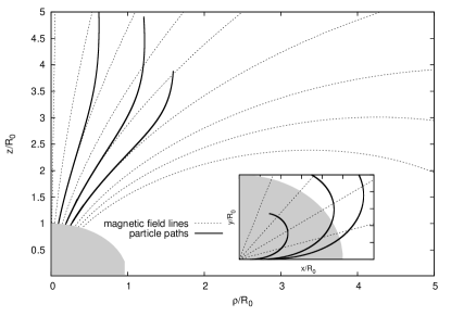
Figure 2: On the left hand side: the proton’s trajectory for initial angles relative the rotation axis $\theta/\theta_{pc}=0.3,\,0.4,\,0.6$ and $B_{15}$, $P_{-3}$ ($\theta_{pc}=27.25^{\circ}$). $\theta_{pc}$ is the angular size of the polar cap. On the right hand side: the time dependence of the relative altitude of protons above the surface of the neutron star for different values of $B$ and $P$.

The path of a proton is shown for ($B_{15},\,P_{-3}$) and different initial angles $(\Theta)$ measured relative to axis of the magnetic dipole on the left hand side of Fig. 2. It can be seen that the proton moves initially nearly along the magnetic field lines when the acceleration process begins, then shoves off the field lines at about $z=2$–$3\,R_{0}$ and finally moves on a helical trajectory along the z-axis far away from the surface.

On the top of the left hand side of Fig. 3, one can see that the maximum proton energy is almost independent of the initial angle when ($B_{15},\,P_{-3}$). This is also true in case of other values of $B$ and $P$ and also valid for the intensity maximum of the radiations as well. Therefore we only plotted the time dependence of the momenta and the power of radiations corresponding to $\theta=0.5\theta_{pc}$ (except the top left of Fig. 3).

It’s interesting to observe time lags in the growth of both momentum components parallel/perpendicular ($\gamma_{\parallel}/\gamma_{\perp}$) to the field lines as can be seen on the top of Fig. 3 and on the right hand side of Fig. 2, in which the time dependence of the relative altitude ($(r-R_{0})/R_{0}$) of protons is shown. In this time region, the proton path is closer to circular ($\gamma_{\perp}\gg\gamma_{\parallel}$) and remains roughly constant because synchrotron radiation loss keeps pace with the transverse energy gain due to acceleration along the field. Then, the path changes to being more elongated due to the increasing electric field ($|\vec{E}_{unsat}|\sim(r-R_{0})/R_{0}$), resulting in a change of the effective radius of curvature. This change of the path is indicated by a jump of the value of $\chi=\gamma/R_{c}$ (at $\approx 10^{-10}$ s) which can be seen in Fig. 4, where we plotted the transverse momentum carried by the transfers of radiations ($k_{\perp}\approx m\chi^{1/3}$). Between $10^{-10}-10^{-7}$ s $\gamma_{\perp}$ is approximately constant and the effect from the proton energy gain is practically compensated by a decrease in the effective curvature radius, so the radiation rate is approximately constant (see the bottom parts of Fig. 3 and Fig. 4). The increase in radiation rate after $10^{-7}$ s is due to the effective radius of curvature starting to decrease more slowly than the proton gains energy, until the saturated regime is reached where energy gains balance energy losses.

From the bottom parts of Fig. 3, one can see that the $\pi_{0}$ radiation is irrelevant, moreover the charged pion radiation intensity becomes comparable to that of the photon radiation only in case of ($B_{15}$, $P_{-3}$).

In Fig. 4, one can see that the transverse momentum transfer of the radiation is small comparing to the total energy both for protons and for constituent protons of Fe ions. It supports the selfconsistency of our softness assumption for the radiation process implicit in our choice of the effective pion–nucleon interacton. However, $k_{\perp}$ is large enough to fragment the ions at the beginning of the trajectory as we noticed in the previous sections.

The results of the numerical solution tell us that the protons can reach energies up to $\approx 10^{9}$/$10^{10}$ GeV in the examined range of B and P. This is in good agreement with the results of the previous section where we compared the cooling time curves to the acceleration time curve. This conclusion is apparently not sensitive to the fact that the value of the momentum perpendicular to the magnetic field lines is almost the same order of magnitude as the parallel component due to the essential presence of perpendicular components of the electric field. We also saw that for ($B_{15},\,P_{-3}$) or higher B and/or lower P it is the charged pion radiation which prompts the energy saturation of the protons (this is consistent with the conclusions obtained from the comparison of the characteristic timescales).

4 Curvature Pion Neutrino Luminosity

In terms of the Goldreich-Julian charged particle density $n_{GJ}=(B/ecP)=7\times 10^{13}B_{15}P^{-1}\hbox{cm}^{-3}$ for a pulsar or magnetar of radius $a$ and period $P$ s, with a polar cap solid angle $\Omega_{p}=\pi\theta_{p}^{2}\sim(2\pi^{2}a/cP)=6.5\times 10^{-4}a_{6}P^{-1}$ sr, the outflow rate of ions with charge $Z$ is

$${\dot{N}_{i}}=a^{2}\Omega_{p}n_{GJ}Z^{-1}c\simeq 1.4\times 10^{33}B_{15}a_{6}^{3}Z^{-1}P^{-2}~{}~{}{\rm s}^{-1}~{}.$$ (21)

For a $\pi^{+}$ radiation efficiency $\eta_{\pi}$ at the ion terminal Lorentz factor, the resulting number of pion-decay $\nu_{\mu}$ and subsequent muon-decay ${\bar{\nu}}_{\mu}$ is 2 per proton, giving for a pulsar at distance $D=10$ Kpc a $\nu_{\mu}$ or ${\bar{\nu}}_{\mu}$ flux at Earth of

$$\Phi_{\nu,c}=Z{\dot{N}_{i}}/4\pi D^{2}\simeq 1.2\times 10^{-13}\eta_{\pi}B_{15}P^{-2}a_{6}^{3}D_{10}^{-2}~{}\hbox{cm}^{-2}\hbox{s}^{-1},$$ (22)

where the label $c$ denotes the curvature pion origin. The corresponding arrival rate in a detector of area $A=1A_{0}$ km² is ${\dot{N}_{\nu}}=\Phi_{\nu}A\simeq 3.7\times 10^{4}\eta_{\pi}B_{15}a_{6}^{3}P^{-2}A_{0}D_{10}^{-2}$ km^-2 yr^-1.

The typical energy of the muon neutrinos is determined by the energy losses incurred by the pions and muons before the decay. As the pions move out to radii comparable to the light cylinder, the $\pi^{+}$ Klein-Nishina energy losses are less important than the $\pi^{+}$ photon curvature losses, which occur on a timescale $t_{c,\pi}\sim 1.2\times 10^{-12}\epsilon_{9\pi}^{-3}a_{6}P_{-3}$ s, where $\epsilon_{9\pi}=(\epsilon_{\pi}/10^{9}\hbox{GeV})$ is the pion energy normalized to $10^{9}$ GeV, while the $\pi^{+}$ decay time is $t_{d,\pi}\sim 1.86\times 10^{2}\epsilon_{9\pi}$ s. The pions cool by curvature radiation until reaching the light cylinder at $t_{L}\sim 1.7\times 10^{-4}P_{-3}$s, where their energy has dropped to $\epsilon_{9\pi L}\sim 1.9\times 10^{-3}a_{6}^{1/3}$. Thereafter the pions move in the wind zone in essentially ballistic paths, cooling adiabatically on a timescale $t_{ad,\pi}=t_{L}(\epsilon_{\pi L}/\epsilon_{\pi})^{3/2}=1.4\times 10^{-8}P_{-3}a_{6}^{1/2}\epsilon_{9\pi}^{-3/2}$ s. The pions decay when their energy reaches $\epsilon_{9\pi d}\simeq 0.89\times 10^{-4}P_{-3}^{2/5}a_{6}^{1/5}\sim 10^{5}$ GeV. The corresponding $\nu_{\mu}$ has an energy $\epsilon_{\nu_{\mu}}\sim\epsilon_{9,\pi,d}/3\sim 33P_{-3}^{2/5}a_{6}^{1/5}$ TeV. The associated $\mu^{+}$ starts with (2/3) of the decaying pion energy and is subject to adiabatic losses. It decays on a timescale $t_{\mu d}\sim 1.97\times 10^{4}\epsilon_{9\mu}$ s, where $\epsilon_{9\mu}$ is the muon energy normalized to $10^{9}$ GeV, reaching at decay an energy $\epsilon_{9\mu d}\simeq 1.08\times 10^{-5}P_{-3}^{2/5}a_{6}^{8/25}\sim 10^{4}$ GeV. The associated muon neutrino has an energy $\epsilon_{\nu_{\mu}}\sim(\epsilon_{9,\mu,d}/3)\sim 3.3$ TeV.

The neutrino event rate in the detector, however, depends on the mixing of neutrino flavors because of oscillations while traveling from their source to Earth. Since the muon neutrinos from pion and muon decays are in two different energy regimes (33 and 3.3 TeV, respectively), one may consider their flavor oscillations independently. With a production flux ratio of $\nu_{e}$:$\nu_{\mu}$:$\nu_{\tau}$=0:1:0, for pion decay $\nu_{\mu}$, the observed ratio would be 0.2:0.4:0.4. For 3.3 TeV muon decay neutrino fluxes, with a production ratio of 1:0:0 and 0:1:0, respectively for $\nu_{e}$ and ${\bar{\nu}}_{\mu}$, the respective observed ratios would be 0.6:0.2:0.2 and 0.2:0.4:0.4. Since the neutrino detectors cannot distinguish between a muon neutrino and an anti-neutrino, the observed flux of 3.3 TeV muon neutrino would be a factor 0.6 times the production flux. The probability per $\nu_{\mu}$ of resulting in an upward muon is $P_{\nu\to\mu}\sim 1.3\times 10^{-6}(\epsilon_{\nu_{\mu}}/\hbox{TeV})$, which for the 33 and 3.3 TeV neutrino cases lead to upward muon count rates from curvature pions, after taking into account oscillation effects, of

$${\dot{N}}_{\mu,c}\simeq\begin{cases}6.3\times 10^{5}\eta_{\pi}B_{15}P_{-3}^{-8/5}a_{6}^{10/3}A_{0}D_{10}^{-2}(\epsilon_{\nu_{\mu}}/33\hbox{TeV})~{}\hbox{km}^{-2}\hbox{yr}^{-1},\cr 9.5\times 10^{4}\eta_{\pi}B_{15}P_{-3}^{-8/5}a_{6}^{10/3}A_{0}D_{10}^{-2}(\epsilon_{\nu_{\mu}}/3.3\hbox{TeV})~{}\hbox{km}^{-2}\hbox{yr}^{-1},\end{cases}$$ (23)

for an on-beam magnetar at 10 Kpc.

In the case of proton acceleration, from Fig. 1 these would reach a maximum energy determined by $\pi^{+}$ curvature losses for fields $B\lower 4.0pt\hbox{$\buildrel>\over{\sim}$}10^{15}$ G and $P\sim 10^{-3}$ s, or $B_{15}P_{-3}^{-2}\lower 4.0pt\hbox{$\buildrel>\over{\sim}$}1$. In these cases $t_{\pi^{+}}\lower 4.0pt\hbox{$\buildrel<\over{\sim}$}t_{c}$ and the $\pi^{+}$ radiation efficiency $\eta_{\pi}\sim 1$, so the upward muon event rate should be detectable in the 1-100 TeV range with cubic kilometer detectors, if the pulsars is on-beam and $B_{15}P_{-3}^{-8/5}A_{0}D_{10}^{-2}\lower 4.0pt\hbox{$\buildrel>\over{\sim}$}10^{-4}$, e.g. for sources in the local group. On the other hand, for values $B_{15}P_{-3}^{-2}<1$, the pion efficiency is low, $\eta_{\pi}\sim t_{c}/t_{\pi}<1$, which would allow potentially detectable neutrino fluxes for sources in our own galaxy provided $\eta_{\pi}\lower 4.0pt\hbox{$\buildrel>\over{\sim}$}10^{-4}-10^{-5}$. For $B_{15}P_{-3}^{-2}\ll 10^{-5}$, the steep behavior of the pion radiation efficiency implies an unobservably small number of events, even for galactic sources. Thus, there is a small range of magnetar field strengths $B_{15}\lower 4.0pt\hbox{$\buildrel>\over{\sim}$}1$ and (short) periods $P_{-3}\sim 1$ for which these objects could be potentially detectable neutrino targets.

5 Photomeson Neutrinos, Cosmic Rays and Photons

Another mechanism for neutrino production in the polar caps is the photomeson process $p\gamma\to\pi^{+}\to\mu^{+}\nu_{\mu}\to e^{+}\nu_{e}{\bar{\nu}}_{\mu}$, acting on the magnetar surface X-rays, typically $L_{x}\sim 10^{35}L_{35}$ erg s^-1 (Zhang et al, 2003). The photon number density near the surface is $n_{\gamma,a}=1.8\times 10^{21}L_{35}^{3/4}$ cm^-3, and for protons of energy much above the threshold $\epsilon\gg 0.1-0.2$ GeV, the cross section $\sigma_{p\gamma}\sim 10^{-28}$ cm² implies a mean interaction time $t_{p\gamma}\simeq 1.8\times 10^{-4}L_{35}^{-3/4}$ s, a mean free path $\ell_{p\gamma}\sim 5\times 10^{6}L_{35}^{-3/4}$ cm, or an optical depth $\tau_{p\gamma}\sim 0.18L_{35}^{3/4}a_{6}$. For $L_{35}\lower 4.0pt\hbox{$\buildrel>\over{\sim}$}1$ and any but the fastest rotating pulsars, the photomeson interaction occurs on a length comparable or less than the light cylinder $R_{L}=5\times 10^{6}P_{-3}$ cm, but much larger than the height $h$ where acceleration balances pion or photon curvature losses.

If the pion curvature process is inefficient, $\eta_{\pi}\ll 1$, most of the protons survive beyond $h$, and inside the light cylinder they cool due to curvature radiation (or outside the light cylinder due to adiabatic cooling), until the photomeson process leads to a neutron and a $\pi^{+}$ which takes $0.2$ of the remaining proton energy. The pions and the subsequent muons then cool due to curvature (if inside $R_{L}$) and adiabatic (when outside $R_{L}$) losses in a similar way as in the previous section. For typical parameters, the average neutrino energy is $<\epsilon_{\nu_{\mu}}>\simeq 28P_{-3}^{3/5}L_{35}^{-3/20}a_{6}^{1/5}$ TeV, not much different from the value $\sim 18P_{-3}^{2/5}a_{6}^{8/25}$ TeV in the pion curvature initiated case of last section, since both the protons (before undergoing $p\gamma$) and the charged pions cool by photon curvature radiation inside the light cylinder, and adiabatically outside. The neutrino flux resulting from $p\gamma$ are larger, for $\tau_{p\gamma}\sim 0.2\gg\eta_{\pi}$, and since the typical neutrino energies from $p\gamma$ are typically only $\sim 2$ larger than in the pion curvature case, in this $\eta_{\pi}\ll 1$ limit it would be hard to distinguish the pion curvature component from the dominant $p\gamma$ flux.

The situation is different for large $\eta_{\pi}\to 1$. In this case it is mainly neutrons that propagate outwards beyond $h$. Being neutral, they do not suffer adiabatic losses, and undergo photopion interactions $n\gamma\to\pi^{-}$ on a timescale similar to protons, $t_{n\gamma}\simeq 1.8\times 10^{-4}L_{35}^{-3/4}$ s. Typically this occurs inside or at the light cylinder. We take as a limiting example the case where this occurs near the light cylinder. The negative pions and muons then undergo adiabatic cooling outside $R_{L}$ similarly to their positive counterparts, as discussed previously, resulting in ${\bar{\nu}}_{\mu}$. Ignoring the distinction between ${\bar{\nu}}_{\mu}$ and $\nu_{\mu}$, which cannot be discriminated in Cherenkov detectors, the resulting average neutrino energy is now $<\epsilon_{\nu_{\mu}}>\sim 280L_{35}^{-3/10}\epsilon_{9ni}^{3/5}$ TeV, where $\epsilon_{9ni}=(\epsilon_{n}/10^{9}\hbox{GeV})$ is the initial neutron energy. The flux is $\Phi_{\nu n\gamma}\sim 5\times 10^{-8}P_{-3}^{-2}B_{15}a_{6}^{4}L_{35}^{3/4}D_{10}^{-2}~{}\hbox{cm}^{-2}\hbox{s}^{-1}$ around $\epsilon_{\nu}\sim 280$ TeV from $n\gamma$ interactions, and the upward muon event rate, modulo the factors due to oscillation effect as previously discussed, is

$${\dot{N}}_{\mu,n\gamma}\simeq 5.4\times 10^{6}B_{15}P_{-3}^{-2}a_{6}^{4}L_{35}^{9/20}A_{0}D_{10}^{-2}(\epsilon_{\nu_{\mu}}/280\hbox{TeV})~{}\hbox{km}^{-2}\hbox{yr}^{-1},$$ (24)

for an on-beam magnetar at 10 Kpc, from $n\gamma$ interactions. The corresponding pion curvature neutrinos would lead to an upward muon event rate given by equation (23), which is not too different. If observed, the difference in the average neutrino energies from pion curvature ($\sim 18$ TeV) and from $n\gamma$ interactions ($\sim 280$ TeV) could help discriminate between the pion curvature and the photomeson production mechanisms. If there were such milisecond magnetars with $\eta_{\pi}\to 1$ in our galaxy ($D\lower 4.0pt\hbox{$\buildrel<\over{\sim}$}10$ Kpc) this would imply, from eqs. (23, 24) upward muons event rates which would be strong in a completed cubic kilometer detector, and probably even in partially completed installations, so the current presence of such objects in our galaxy is questionable.

These ${\vec{\Omega}\cdot\vec{B}}<0$ caps will also result in a significant flux of escaping neutrons, which contribute to the cosmic ray flux. As an example, taking the case for the efficiency of $\pi^{+}$ radiation by protons from magnetars with $B_{15}P_{-3}^{-2}=1$, for which $\eta_{\pi}\simeq t_{\pi^{+}}/t_{c}\sim 0.2$, the flux of neutrons at Earth and their energies are

$$\Phi_{n}\simeq 10^{-11}B_{15}P_{-3}^{-2}D_{10}^{-2}~{}{\rm m}^{-2}~{}{\rm s}^{-1}~{}{\rm sr}^{-1}~{}~{};~{}~{}\epsilon_{n}\simeq 6\times 10^{17}~{}{\rm eV}~{}.$$ (25)

A neutron of $6\times 10^{17}$ eV energy decays after traveling $\sim 6$ kpc. For comparison, the observed cosmic-ray number flux at this energy is $\approx 9\times 10^{-12}~{}{\rm m}^{-2}~{}{\rm s}^{-1}~{}{\rm sr}^{-1}$ (Nagano & Watson, 2000). However, the very small degree of observed cosmic ray anisotropy at these energies again suggests that the probability of finding such $\eta_{\pi}\to 1$ magnetars within our galaxy at any given time is very low.

In the case of a newly born neutron star or magnetar, the escaping neutrons may interact with the expanding supernova-remnant (SNR) shell, as discussed by Razzaque, Mészáros & Waxman (2003). For a hypernova which results in a magnetar, the shell speed is $v=10^{10}v_{10}$ cm/s and reaches a radius $R_{snr}\simeq 8.6\times 10^{14}v_{10}t_{d}$ cm in $t_{d}$ days. With a typical shell mass of $M_{snr}=2\times 10^{33}m_{snr}$ g, the column density of target atoms is $\Sigma_{A}\simeq 1.3\times 10^{26}m_{snr}t_{d}^{-2}v_{10}^{-2}~{}{\rm cm}^{-2}$. The $pp$ cross-section for $\sim 10^{18}$ eV energy incident neutrons is 100 mb and the corresponding optical depth is $\tau_{pp}\sim 10m_{snr}t_{d}^{-2}v_{10}^{-2}$. The energy of the neutrinos produced by a $7\times 10^{17}$ eV neutron via $pp$ interactions ranges from $\sim m_{\pi}c^{2}\gamma_{cm}/4\simeq 0.7$ TeV up to $\sim\epsilon_{n}/4$ with a $\epsilon_{\nu}^{-1}$ distribution normalized to a multiplicity of $10^{-3}$ at this energy (Razzaque, Mészáros & Waxman, 2003). Here $\gamma_{cm}$ is the Lorentz factor of the center-of-mass of the $pp$ interaction in the Lab frame.

There may also be photo-hadronic interactions with photons in the SNR shell created from the SN explosion. The peak energy of these blackbody photons at creation is $\approx 18.2E_{51}^{1/4}r_{11}^{3/4}$ keV for $\sim 10^{51}E_{51}$ erg SN explosion energy and $\sim 10^{11}r_{11}$ cm progenitor star’s radius. In the SNR shell, however, they cool down to a peak energy of $\epsilon_{\gamma,sn}\simeq 2.1E_{51}^{1/4}r_{11}^{1/4}v_{10}^{-1}t_{d}^{-1}$ eV. Thus neutrons of $\gtrsim 10^{17}$ eV energy may produce pions by interacting with them. Assuming that the total number of SN photons do not change after their creation, the column density of them in the SNR shell is $\Sigma_{\gamma,sn}\simeq 3.65\times 10^{27}E_{51}^{3/4}r_{11}^{3/4}v_{10}^{-2}t_{d}^{-2}~{}{\rm cm}^{2}$ and the opacity for photo-hadronic interactions is $\lesssim 1$ with 0.1 mb typical cross-sections at the resonances. The resulting neutrino energy in this case would be in the 10’s of PeV range. There may be additional components of VHE ions accelerated in the SNR shell or the outer-gaps of a pulsar/magnetar which could also interact with the SNR shell (Guetta & Granot, 2003). These interactions will produce additional neutrinos and hence identifying the neutrinos from pion curvature radiation may be difficult for $t\lower 4.0pt\hbox{$\buildrel<\over{\sim}$}$ few days after a magnetar is born.

Ultra-high energy photons will also be produced, both through curvature radiation of charged pions and muons, and through decay of the associated neutral pions. E.g. pions produced by $\sim 10^{9}$ GeV protons would lead to pion-related UHE photons of luminosity $L_{\gamma(\pi)}\sim 10^{44}B_{15}P_{-3}^{-2}a_{6}^{3}$ erg s^-1, decaying as the field drops and the period lengthens. The curvature photon energy is $\epsilon_{\gamma}\sim 3P_{-3}^{-2}a_{6}^{-1/2}(\epsilon_{\pi}/10^{8}\hbox{GeV})^{3}$ PeV. These, as well as the muon curvature and neutral pion decay photons are all well above the $2m_{e}c^{2}/\sin\theta$ threshold for one-photon pair production $\gamma B\to e^{\pm}$ (e.g. Harding and Lai, 2006), where $\theta$ is the angle of propagation relative to field direction. The optical depth above threshold for a path length $10^{6}R_{6}$ cm is $\tau_{\gamma B}\sim 5\times 10^{10}(B_{15}^{2/3}\sin\theta)^{2/3}R_{6}(\epsilon_{\gamma}/\hbox{PeV})^{-1/3}$. (Another UHE photon opacity is photon splitting, a higher order mechanism which above threshold is less important than one-photon pair formation). The UHE photons will thus be degraded to energies below the threshold, $\epsilon_{\gamma}\lower 4.0pt\hbox{$\buildrel<\over{\sim}$}10~{}\theta_{-1}^{-1}$ MeV, for cap angles $\theta\sim 10^{-1}\theta_{-1}$.

6 Discussion

Our discussion has assumed that the properties of the inner gaps near the polar caps of pulsars or magnetars allow protons to be accelerated to energies $\lower 4.0pt\hbox{$\buildrel>\over{\sim}$}6\times 10^{8}$ GeV. This is an open question, since the extent and properties of polar gaps (with ${\vec{\Omega}}\cdot{\vec{B}}\leq 0$) including self-consistently pion radiation effects is unknown. Such studies, if undertaken, would have to take into account not only the effects of leptons acceleration from charged pion decays, but also high energy photons from neutral pion decay and their subsequent cascades. Studies of space charge limited gaps with electron acceleration and pair production (e.g. Harding and Muslimov, 2002; also Baring and Harding, 2002) suggest that Lorentz factors of order $10^{9}$ may be possible in fast-rotating, high field objects, in which case the effects discussed here may become important.

The curvature pion radiation mechanism is likely to be of interest for fast rotating magnetars which accelerate protons. This is because, from Fig. 1, we see that for magnetic field and period values $B_{15}P_{-3}^{-1}\lower 4.0pt\hbox{$\buildrel>\over{\sim}$}1$ the pion curvature radiation dominates the photon curvature radiative cooling. For such magnetic field and period combinations, the acceleration of heavy ions results in the fragmentation of the ions before pion emission occurs, which is expected only from the individual protons resulting from the fragmentation after they have been further accelerated.

There is so far no observational evidence for millisecond periods among the handful of known magnetars (e.g. Kaspi, 2007; Woods and Thompson, 2004), most of which are in our galaxy and have periods of seconds. From eq. (23), we see that for $B\lower 4.0pt\hbox{$\buildrel>\over{\sim}$}10^{15}$ G and millisecond periods, the muon event rate is so large that they might have been detected by now, if the magnetar were on-beam and at a distance $D\lower 4.0pt\hbox{$\buildrel<\over{\sim}$}$ Mpc. The likeliest explanation is that such millisecond magnetars do not exist in our galaxy (or else they might be off-beam). At the same time, it is reassuring that for periods $P\lower 4.0pt\hbox{$\buildrel>\over{\sim}$}1$ s the pion curvature efficiency predicted is $\eta_{\pi}=t_{c}/t_{\pi}\lll 1$, and the corresponding muon event rate in cubic kilometer detectors given by equation (23) is negligible for known galactic magnetars.

An interesting possibility is that some fraction of core collapse supernovae lead, at least initially, to a millisecond magnetar. There is currently no observational evidence for this, but it is a plausible hypothesis, among others from fast convective overturn dynamo arguments, e.g. Thompson and Duncan (1996). In such objects, the envelope optical thickness to $\nu N$ interactions is $\tau_{\nu N}\sim 10^{-6}(\epsilon_{\nu}/\hbox{10 TeV})(M_{env}/10M_{\odot})(v_{env}/0.1c)^{-2}(t/\hbox{day})^{-2}$, and as long as the magnetic field and the rotation rate remain high, neutrinos produced by pion curvature and $p\gamma$ interactions can escape without further reprocessing. Thus, core collapse supernovae which result initially in a millisecond magnetar with $B\lower 4.0pt\hbox{$\buildrel>\over{\sim}$}10^{15}$ G are expected to undergo a brief period of intense pion and ultra-high energy neutrino production, which significantly exceeds any electromagnetic energy losses. If the fraction of core collapse supernovae leading to such objects were $0.05-0.1$, given the frequency of core collapse SNe in the LMC and in the local group, one could in principle expect some millisecond magnetars detectable in cubic kilometer detectors within timescales of years. In this scenario one would also expect (§5) a significant $\lower 4.0pt\hbox{$\buildrel<\over{\sim}$}10$ MeV photon luminosity, which may be detectable by the GLAST GBM.

In summary, we have pointed out that pions produced by protons interacting with the curved strong magnetic fields of magnetars may be an important energy loss mechanism for the accelerated particles, leading to secondary leptons and photons which can affect the properties of the inner gaps. Our model for the strong interaction processes involved here relies on the softness of the pion radiation process. Although the correctness of this assumption needs further, more detailed investigation, this level of approximation is justifiable here, given the larger uncertainties in the astrophysical model. Our results indicate that the effects analysed in this paper could lead to copious neutrino production in the TeV-nPeV range, which would provide interesting targets for cubic kilometer scale detectors.

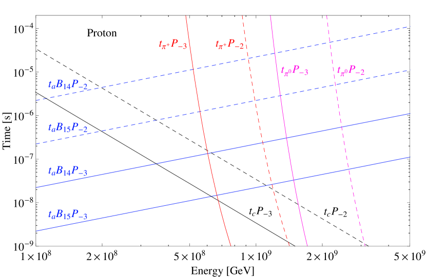
Figure 1: Energy loss timescales $t_{\pi^{+}}$ and $t_{\pi^{0}}$ for proton curvature emission of $\pi^{+}$ and $\pi^{0}$, compared to photon curvature radiation loss timescale $t_{c}$ and acceleration time $t_{a}$, as a function of proton energy (in GeV), for different field strengths $B=10^{15}B_{15}$ (G) and periods $P=10^{-3}P_{-3}$ (s).

Figure 3: Acceleration of protons. The parallel and perpendicular momenta for $B_{15}$, $P_{-3}$ (a), and for $B_{15}$, $P_{-2}$ ($\theta_{pc}=8.33^{\circ}$) and $B_{14}$, $P_{-3}$ ($\theta_{pc}=27.25^{\circ}$) where $\theta=0.5\theta_{pc}$ (b). The intensity of each type of radiation for $B_{15}$, $P_{-3}$ (c), for $B_{14}$, $P_{-3}$ and $B_{15}$, $P_{-2}$ (d) where $\theta=0.5\theta_{pc}$. The vertical lines indicate the switch between the unsaturated and saturated fields.

Figure 4: Transverse momentum transfer the radiations from protons (left hand side) and constituent protons of Fe ions (right hand side) along the path. The photon radiation dominates in case of ($B_{15},\,P_{-2}$) and ($B_{14},\,P_{-3}$), and in case of ($B_{15},\,P_{-3}$) up to $t\approx 10^{-6}$s.

References

- (1) Arons, J., 2002, ApJ, 589:871
- (2) Baring, M. and Harding, A.K., 2002, talk at HEAD meeting, Albuquerque, NM.
- (3) Berezinsky, V., Dolgov, A. and Kachelriess, M., 1995, Phys. Lett. B351, 261.
- (4) Blasi, P., Epstein, R.I. andf Olinto, A., 2000, ApJ (Lett.), 533:L123
- (5) Ginzburg, V.L. and Zharkov, G.F., 1964, Sov. JETP (Lett.), 47, 2279
- (6) Goldreich, P. and Julian, W.H., 1969, ApJ 157, 869
- (7) Guetta, D. and Granot, J., 2003, Phys. Rev. Lett. 90, 201103
- (8) Harding, A.K. and Lai, D., 2006, Rep. Prog. Phys., 69:2631
- (9) Harding, A.K. and Muslimov, A.G., 2001, ApJ 556, 987.
- (10) Harding, A.K. and Muslimov, A.G., 2002, ApJ 568, 862.
- (11) Harding, A.K., Usov, V.V. and Muslimov, A.G., 2005, ApJ 622, 531.
- (12) Herpay, T. and Patkós, A., 2008, J. Phys. G: Nucl. and Part. Phys. 35:025201
- (13) Kaspi, V., 2007, Astrophysics and Space Science, in press (arXiv:astro-ph/0610304)
- (14) Medin, Z. and Lai, D., 2007, MNRAS, 382:1833
- (15) Medin, Z. and Lai, D., 2008, AIP Conf. Proc. 983, 249
- (16) Nagano, M. and Watson, A.A., 2000, Rev.Mod.Phys. 72:689
- (17) Razzaque, S., Mészáros , P. and Waxman, E., 2003, Phys. Rev. Lett. 90, 241103
- (18) Ruderman, M. and Sutherland, P.G., 1975, ApJ 196:51
- (19) Sutherland, P.G., 1979, Fundamentals of Cosmic Physics 4, 95
- (20) Takata, J. et al., 2008, MNRAS, in press arXiv:0801.1147v1[astro-ph]
- (21) Thompson, C. and Duncan, R.C., 1996, ApJ,473:322
- (22) Thompson, C., 2008, arXiv:0802.257 [astro-ph]
- (23) Tokuhisa, A. and Kajino, T., 1999, ApJ, 525, L117.
- (24) Woods, P.M. and Thompson, C., 2004, in “Compact Stellar X-ray Sources”, Eds. W.H.G. Lewin and M. van der Klis (Cambridge: CUP) (arXiv:astro-ph/0406133)
- (25) Zhang, B., et al, 2003, ApJ 595:346
- (26) Zharkov, G.F., 1965, Sov. J. Nucl. Phys. 1, 173