Efficiency of Rejection-Free Methods for Dynamic Monte Carlo Studies of Off-lattice Interacting Particles

Abstract

We calculate the efficiency of a rejection-free dynamic Monte Carlo method for $d$-dimensional off-lattice homogeneous particles interacting through a repulsive power-law potential $r^{-p}$. Theoretically we find the algorithmic efficiency in the limit of low temperatures and/or high densities is asymptotically proportional to $\rho^{\tfrac{p+2}{2}}T^{-\tfrac{d}{2}}$ with the particle density $\rho$ and the temperature $T$. Dynamic Monte Carlo simulations are performed in 1-, 2- and 3-dimensional systems with different powers $p$, and the results agree with the theoretical predictions.

I Introduction

Since their introduction in 1953 Metropolis et al. (1953) classical Monte Carlo (MC) methods mave matured into a useful tool for studying many different phenomena in different fields such as material science, high energy physics, and biology Binder (1979); Miyashita and Takano (1980); Binder (1997). For the study of the statics of a given model, the MC method can be viewed as a probabilistic method of performing multi-dimensional integrals Press et al. (1986) that could correspond to the partition (or grand partition) function of the model Binder (1979). Various methods to increase the efficiency or accuracy of the method exist, including importance sampling Binder (1979), which allows the MC method to provide an estimate for the ratio of two integrals, for example to give an estimate of the average energy $\langle E\rangle$ of the system. Other advanced algorithms, such as Swendsen-Wang or cluster algorithms Binder (1979); Landau and Binder (2005), can also be used to alleviate difficulties associated with critical slowing down near $T_{c}$ or being frozen into valleys for $T<T_{c}$. All of these advanced methods are allowed because they provide estimates for the underlying integral(s) in an efficient fashion. For any of these MC methods, the system to be studied is in some configuration, which has a particular energy $E_{i}$, and an algorithm to obtain a new configuration $j$ from configuration $i$ is implemented. For $M$ generated configurations, the estimate for the average energy is given by $\langle E\rangle=\frac{1}{M}\sum_{i=1}^{M}E_{i}$.

If one is interested in the physical time evolution of a model system, the MC method can still be used. Although in principle any MC algorithm for statics could be used to study the time development through phase space of the model system, only certain MC methods will correspond to the actual time evolution of the system being modeled. In other words, many of the methods mentioned above, such as Swendsen-Wang or cluster algorithms Binder (1979); Landau and Binder (2005), change the rate at which the system moves through phase space and consequently would usually not be associated with the actual time development of the physical system. The older MC literature simply refers to the method as a MC method (see the references in Sec. 3.4 of Ref. Binder (1997)), even when the time development of the MC algorithm is assumed to correspond to that of the actual model system Stoll et al. (1973). More recently, use of MC methods to study the physical time dependence of a model system has been called either dynamic MC or kinetic MC. Although these two terms are sometimes used interchangably, there is an emerging distinction between them. Kinetic MC has become the standard name for the case where physical time development is studied with known rate constants for the system to evolve from one state to another Voter (2007). These rate constants may be approximated under certain assumptions (such as applicability of transition state theory to atomistic systems) using ab initio methods Voter (2007). (Use of rate constants also allows the transition from discrete MC steps to continuous time.) However, there are other instances where the physical time evolution of the system is desired while rate constants might be unavailable (for example perhaps transition state theory does not apply or an important complicated multi-particle motion might be difficult to conceptualize or calculate). In such cases the physical time development may sometimes still be derived from the underlying physical system, for example by studying the underlying quantum mechanism for time development Martin (1977); Park et al. (2002, 2004); Park (2008), or devising a method equivalent to the time development of the underlying equations Cheng et al. (2006, 2007).

Such studies, which we concentrate on in this article, are called dynamic MC studies to distinguish them from static (equilibrium) MC or from kinetic MC studies. Thus we use the term dynamic MC in the same way as the recent book by Krauth Krauth (2006).

Frequently in dynamic simulations we need to work with long time scales at very low temperatures or in a strong external field. In these cases the standard dynamic MC method becomes very inefficient due to the high rejection rate which requires a large number of trial moves before a change is made to the state of the system. Most advanced algorithms, such as Swendsen-Wang or cluster algorithms Binder (1979); Landau and Binder (2005), change the dynamic of the system thereby changing the time development of the system, which makes it impossible to study systems where the MC move is based on physical processes. The rejection-free MC (RFMC) method was proposed to overcome this problem with standard dynamic MC. The RFMC was first applied to discrete spin systems Bortz et al. (1975); Gillespie (1976, 1977) including the kinetic Ising Model Miyashita and Takano (1980). It was later generalized to classical spin systems with continuous degrees of freedom Muñoz et al. (2003). The RFMC method allows us to efficiently simulate a system with a high rejection rate without any changes of the original dynamics, since it shares the original Markov chain with the standard dynamic MC method. The RFMC method in this paper is very similar to the method labeled ‘faster-than-the-clock algorithm’ in Ref. Krauth (2006).

The RFMC requires, to proceed by one algorithmic step, the values of all the probabilities of choosing a new state. Therefore, the computational cost of one step is larger than that of the standard MC. For this reason it is necessary to have a method to calculate its efficiency on a particular problem without implementing the method directly. Watanabe et al. developed a method Watanabe et al. (2006) to calculate the efficiency of the RFMC for spin systems and hard particle systems. In the present paper, we evaluate the efficiency of the RFMC method for dynamic MC studies of $d$-dimensional particle systems with the particles interacting through a repulsive short-range power law potential. Even though the bookkeeping involved in actually implementing the RFMC method may be substantial, leading to more computer time per algorithmic step than the standard dynamic MC method, at temperatures low enough or fields high enough where rejection rates are extremely high, the RFMC will be more efficient than the standard dynamic MC algorithm.

The paper is organized as follows. In Sec. II, we present a review of the standard dynamic MC algorithm and the RFMC algorithm. In Sec. III, we provide analytical estimates for the efficiency of the RFMC method for repulsive power law potentials. In Sec. IV, we show the results of our simulations in 1, 2 and 3 dimensions. Sec. V is devoted to discussions and conclusions.

II Dynamic Monte Carlo

II.1 Standard Dynamic Monte Carlo

The standard dynamic MC algorithm for particle systems involves the following six iterative steps, with one iteration being called a MC step (MCS). We have used the term dynamic MC for this algorithm, rather than the term time-quantified MC used in Cheng et al. (2006, 2007), since it has been used previously Park et al. (2002, 2004); Park (2008); Krauth (2006). It is important to remember that in dynamic MC the time in MCS is proportional to the physical time in seconds Martin (1977); Park et al. (2002, 2004); Park (2008); Cheng et al. (2006, 2007). The algorithm satisfies detailed balance. It is very similar to the time-quantification of the dynamic MC for Brownian ratchets Cheng et al. (2007).

1. Choose one particle randomly from the $N$ particles, the chosen particle $i$ is located at position ${\vec{r}}_{{\rm old},i}$.

2. Choose a new position of the chosen particle randomly as ${\vec{r}}_{{\rm new},i}={\vec{r}}_{{\rm old},i}+\Delta{\vec{r}}$, with $\Delta{\vec{r}}$ chosen uniformly over a $d$-dimensional hyper-spherical volume

   $$V_{\rm choose}=\frac{\pi^{\frac{d}{2}}\>r_{\rm choose}^{d}}{\Gamma\left(\frac{d}{2}+1\right)}\>,$$ (1)

   with a radius $r_{\rm choose}$ and the gamma function $\Gamma$. The probability density for choosing the new position of the chosen particle is $d^{d}x_{i}/V_{\rm choose}$.

3. Reject the new position if it is located outside the ‘cage’ formed by line segments joining its nearest-neighbor (nn) particles. (In the usual way, the ‘cage’ is defined in this off-lattice simulation on the basis of a Voronoi diagram (or Delaunay triangulation), but can be often equally well defined for our homogeneous high-density systems as particles within a certain distance of the chosen atom Watanabe et al. (2006).)

4. Evaluate the energy difference $\Delta E_{i}=E_{{\rm new},i}-E_{{\rm old},i}$ between the new and the old positions of the chosen particle $i$.

5. Decide whether to accept the trial move by comparing a random number with the move probability which is a function of $\Delta E_{i}$. For example, we can use the Metropolis criteria to choose the transition probability as

   $$P({\vec{r}}_{{\rm new},i}\mid{\vec{r}}_{{\rm old},i})=\left\{\begin{array}[]{cc}1&\text{if~{}}\Delta E_{i}\leq 0,\\ \exp(-\beta\Delta E_{i})&\text{otherwise}.\end{array}\right.$$ (2)

6. If the trial move is accepted, move the particle to its new position, otherwise leave it in its old position.

II.2 Dynamic Monte Carlo Without Rejections

The rejection-free MC (RFMC) method was developed to overcome the decrease in the efficiency of the standard dynamic MC method in cases where the rejection rate is high, for example, in systems at a very low temperature. The efficiency of the standard dynamic MC algorithm is the rate at which it changes the current state of the system, this is the fraction of accepted moves to the total number of move attempts. One algorithmic step of the RFMC involves the following procedures.

1. Compute the time to leave the current state (the waiting time $t_{\text{wait}}$). This is the number of trial states which would be rejected in the standard dynamic MC. Hence in one algorithmic step the time is advanced by $t_{\text{wait}}$.

2. Advance the time of the system by $t_{\text{wait}}$.

3. Calculate probabilities $\lambda_{i}$ for each of the $N$ particles, where $\lambda_{i}$ denotes the probability that the trial move of particle $i$ would be rejected in the standard dynamic MC given that it was the particle chosen for the trail move. Explicitly

   $$\lambda_{i}\>=\>1\>-\>\frac{1}{V_{\rm choose}}\int_{V_{\rm choose}}P({\vec{r}}_{{\rm new},i}\mid{\vec{r}}_{{\rm old},i})d^{d}x_{{\rm new},i}.$$ (3)

4. Then choose a particle with the probability proportional to $1-\lambda_{i}$, that is, the probability that the particle $i$ is chosen is given by $\displaystyle\frac{1-\lambda_{i}}{\sum_{k=1}^{N}(1-\lambda_{k})}$. Therefore, the particle which is easy to move has a higher probability to be chosen.

5. Choose a new position of the chosen particle. This is accomplished using the probability density

   $$\frac{P({\vec{r}}_{{\rm new},i}\mid{\vec{r}}_{{\rm old},i})d^{d}x_{{\rm new},i}}{V_{\rm choose}\left(1-\lambda_{i}\right)}.$$ (4)

The above procedure does not contain any rejection step, and therefore, each RFMC algorithmic step always involves a change of state of the system.

The efficiency of the RFMC method is inversely proportional to the rejection rate of the standard dynamic MC, but they share the same dynamics. Therefore the efficiency of the RFMC is related to the inefficiency of the standard dynamic MC. For this reason the efficiency of the RFMC will be proportional to $t_{\text{wait}}$ which is given by Watanabe et al. (2006); Novotny (1995):

$$t_{\text{wait}}=\biggl{\lfloor}\frac{\ln\tilde{r}}{\ln\Lambda}\biggr{\rfloor}+1.$$ (5)

Here $\tilde{r}$ is a random number uniformly distributed on $(0,1]$, $\lfloor\cdot\rfloor$ is the integer part, and $\Lambda=\frac{1}{N}\sum_{i=1}^{N}\lambda_{i}$ is the probability to stay in the current state (that the move to the trial state will be rejected) after one standard dynamic MC trial move. The units of time are in MCS, but can be quantified with physical time Martin (1977); Park et al. (2002, 2004); Park (2008); Cheng et al. (2006, 2007). We have used the Metropolis method Metropolis et al. (1953) as shown in Eq. (2) in this example and in our simulations in the next section. However, the RFMC algorithm would also work for different functional probabilities such as the Glauber or heat-bath dynamic Binder (1979); Miyashita and Takano (1980); Martin (1977) or a phonon dynamic Park et al. (2002); Park (2008).

III Efficiency of RFMC for Power-law Potentials

Consider $d$-dimensional particles with a repulsive power-law potential and $N_{\rm nn}$ nearest-neighbors (nn) [the particles that form its ‘cage’]. The potential between any two nn particles is

$$V(r)=\left\{\begin{array}[]{cc}\Bigl{(}\displaystyle\frac{\sigma}{r}\Bigr{)}^{p}-\Bigl{(}\displaystyle\frac{\sigma}{r_{0}}\Bigr{)}^{p}&r\leq r_{0}\\ 0&r\geq r_{0}\end{array}\right.$$ (6)

where $r$ is the distance between particles, $p$ is the power, $r_{0}$ is the cut-off distance and $\sigma$ is the length that gives the strength of the interaction, respectively. This potential function represents the hard repulsive core of any potential, such as the Lennard-Jones potential which has $p=12$, and this repulsive part becomes dominant at high densities.

We have chosen the origin of the coordinate system to be at the position of the chosen atom $i$. The energy difference of the atom $i$ is given by $\Delta E_{i}=U_{i}(\vec{x})-U_{i}(\vec{0})$ with $\vec{x}$ the trial position. The efficiency of the rejection-free algorithm at low temperatures and/or high densities is given for the Metropolis dynamic by

$$\bigl{\langle}\exp\left[-\beta\Delta E\right]\bigr{\rangle}=\frac{\Gamma\left(\frac{d}{2}+1\right)}{\pi^{\frac{d}{2}}\>r_{\rm choose}^{d}}\int_{-\infty}^{\infty}\cdots\int_{-\infty}^{\infty}d^{d}x\>\Theta_{\rm cage}\>\exp\left\{-\beta\left[U_{i}(\vec{x})-U_{i}(\vec{0})\right]\right\},$$ (7)

where the interaction energy for particle $i$ is given by the power-law dependence, $p$, of the repulsive part of the interatomic potential

$$U_{i}\left({\vec{x}}\right)=\sum\limits_{N_{\rm nn}}V(r)=\sum_{k=1}^{N_{\rm nn}}\frac{\sigma^{p}}{|\vec{x}-\vec{x}_{k}|^{p}},$$ (8)

with $\vec{x}_{k}$ the position of the $k^{th}$ nn atom of the chosen atom $i$. Here $\Theta_{\rm cage}$ restricts the integrand to be non zero only with the cage formed by the nn particles. The angular brackets denote an average over all allowed states of the system weighted with the Boltzman weight at each configuration. Since we are interested in the system at high densities or at low temperatures, we can utilize the Laplace saddle-point integration approximation Erdelyi (1956)

$$Z_{p}=\int\cdots\int d^{d}xP(\vec{x})\approx P(\vec{x}_{0})\sqrt{\frac{(2\pi)^{d}}{{\rm det}{\bf A}}}$$ (9)

where the integrand $P(\vec{x})$ is strongly peaked around $\vec{x}=\vec{x}_{0}$ and

$$A_{ij}=-\frac{\partial^{2}}{\partial x_{i}\partial x_{j}}\biggl{.}\ln\left[P(\vec{x})\right]\biggr{|}_{\vec{x}=\vec{x}_{0}}.$$ (10)

We assumed the chosen particle is at or near its local energy minimum, i.e., $P\left({\vec{x}_{0}}\right)\approx 1$. Therefore

$$\bigl{\langle}\exp\left[-\beta\Delta E\right]\bigr{\rangle}\approx\frac{\Gamma\left(\frac{d}{2}+1\right)\>T^{\frac{d}{2}}}{\pi^{\frac{d}{2}}\>r_{\rm choose}^{d}}\sqrt{\frac{\left(2\pi\right)^{d}}{\left|{\rm det}\>{\tilde{\bf A}}\right|}},$$ (11)

since after making the derivation in Eq. (10) we get a factor of $\beta$ and the only values that are not 0 are when $i=j$ we have defined $A_{ij}=\beta{\tilde{A}}_{ij}$, and the determinant of ${\bf A}$ is thus proportional to $\beta^{d}$. This immediately gives that the temperature dependence of the average waiting time is proportional to $\beta^{\frac{d}{2}}=T^{-\frac{d}{2}}$.

Furthermore, because of the power-law approximation of Eq. (8), and that two partial derivatives must be taken for the saddle-point approximation $A_{ij}\sim r_{\rm nn}^{-p-2}$ where $r_{\rm nn}$ is the nn distance if all nn atoms are equidistant from the chosen atom. The particle density $\rho$ is proportional to $r_{\rm nn}^{-d}$, and therefore, $\left|{\bf A}\right|^{-\frac{d}{2}}\sim\left[r_{\rm nn}^{-p-2}\right]^{-\frac{d}{2}}\sim\rho^{\frac{-p-2}{2}}$. Equation (7), therefore becomes

$$\bigl{\langle}\exp\left[-\beta\Delta E\right]\bigr{\rangle}\sim\frac{T^{\frac{d}{2}}}{r_{\rm choose}^{d}\>\rho^{\frac{p+2}{2}}},$$ (12)

and the average time between acceptances in the dynamic MC procedure is

$$\left\langle t_{\rm wait}\right\rangle\approx\frac{1}{\left\langle\exp\left[-\beta\Delta E\right]\right\rangle}\sim\frac{r_{\rm choose}^{d}\>\rho^{\frac{p+2}{2}}}{T^{\frac{d}{2}}}.$$ (13)

Equation (13) is the main result of this paper. The result is very general, both for various dimensional particles and for various power laws, as well as being general for the explicit dynamic that is used in the MC procedure.

Throughout the present paper, we assume all the atoms have identical potentials. In the following, we calculate the explicit expression of Eq. (13) for several conditions. For the 1-dimensional system, the average waiting time is given by

$$\left\langle t_{\rm wait}\right\rangle_{d=1}=\frac{2r_{\rm choose}}{r_{\rm nn}^{(p+2)/2}}\sqrt{\frac{\sigma^{p}p(p+1)}{T\>\pi}}\sim\frac{\rho^{\frac{p+2}{2}}}{\sqrt{T}},$$ (14)

since $V_{\rm choose}=2r_{\rm choose}$, $N_{\rm nn}=2$, and

$$\left|{\tilde{\bf A}}\right|=\left|\frac{\partial^{2}\left[U_{i}({\vec{x}})-U_{i}({\vec{0}})\right]}{\partial x^{2}}\right|_{x=0}=\frac{2\sigma^{p}p\left(p+1\right)}{r_{\rm nn}^{p+2}}.$$ (15)

For the 2-dimensional system which has a hexagonal lattice as the ground state, the average waiting time is given by

$$\left\langle t_{\rm wait}\right\rangle_{d=2}=\frac{3\sigma^{p}p^{2}r_{\rm choose}^{2}}{2Tr_{\rm nn}^{p+2}}\sim\frac{\rho^{\frac{p+2}{2}}}{T},$$ (16)

since $V_{\rm choose}=\pi r_{\rm choose}^{2}$, $N_{\rm nn}=6$, and

$$\tilde{A}_{ij}=\left.\frac{\partial^{2}\left[U_{i}({\vec{x}})-U_{i}({\vec{0}})\right]}{\partial x_{i}\partial x_{j}}\right|_{{\vec{x}}=0}=-\delta_{ij}\frac{3\sigma^{p}p^{2}}{r_{\rm nn}^{p+2}},$$ (17)

with the Kronecker delta $\delta_{ij}$. For the 3-dimensional system which has the face-centered-cubic (FCC) lattice as the ground state, the average waiting time is given by

$$\left\langle t_{\rm wait}\right\rangle_{d=3}=\frac{\left[\sigma^{p}p(p-1)\right]^{\frac{3}{2}}\>r_{\rm choose}^{3}}{3\sqrt{\pi}2^{\frac{10+3p}{4}}T^{\frac{3}{2}}r_{\rm nn}^{\frac{3(p+2)}{2}}}\sim\frac{\rho^{\frac{p+2}{2}}}{T^{\frac{3}{2}}},$$ (18)

since $V_{\rm choose}=(4/3)\pi r_{\rm choose}^{3}$, $N_{\rm nn}=12$, and

$$\tilde{A}_{ij}=\left.\frac{\partial^{2}\left[U_{i}({\vec{x}})-U_{i}({\vec{0}})\right]}{\partial x_{i}\partial x_{j}}\right|_{{\vec{x}}=0}=-\delta_{ij}\frac{\sigma^{p}p(p-1)2^{2+\frac{p}{2}}}{r_{\rm nn}^{p+2}}.$$ (19)

Note that, the density and the temperature dependence in a simple-cubic lattice is equivalent to that of Eq. (19), while the coefficient is different since $N_{\rm nn}=6$ and $\tilde{A}_{ij}=-\delta_{ij}\left(\sigma^{p}p(p-1)\right)/r_{\rm nn}^{p+2}$.

IV Simulations in $d$ = 1, 2, and 3

Following the methodology described above, we performed simulations for 1-, 2-, and 3-dimensional systems. The goal is to locate where the asymptotic results of Eq. (13) hold for our RFMC method. The density of the system $\rho$ is defined to be $\rho\equiv N(2a/L)^{d}$, with the number of particles $N$, the radius of the particles $a$, the linear system size $L$, and the dimensionality of the system $d$, respectively. Throughout all the simulations $r_{\text{choose}}$ is set to 0.05 and the cut-off radius $r_{0}$ is set to $r_{0}=1.1r_{nn}(\rho)$, with $r_{nn}(\rho)$ the nearest-neighbor distance for the given density. The simulations were performed for four values of $p$: 2, 4, 6, and 12. For all values of $d$, the density is fixed at $\rho=2.0$ in order to study the temperature dependence, the temperature is fixed at $T=0.001$ to study the density dependence. All simulations were performed starting from the ground state, with periodic boundary conditions, with the simulated volume such that an integer number of unit cells of the ground state fit into the volume.

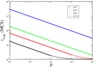
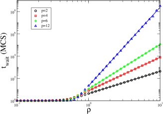
Figure 1: (Color online) (a) Temperature dependence of the average $t_{\text{wait}}$ in $d=1$ for $N=200$ particles, the solid lines are the power law fits. (b) Density dependence of $t_{\text{wait}}$ in $d=1$, the solid lines are power law fits with $\rho\geq 0.6$.

We study the 1-dimensional system with $N=200$ particles which are located on the line of length $L$ with periodic boundary conditions. The temperature dependence of the average for $t_{\text{wait}}$ is shown in Fig. 1 (a), in this case with statistics from $10^{6}$ MCS per particle (MCSp). The power law fit gives $\langle t_{\text{wait}}\rangle\sim T^{-0.49(1)}$ with the correlation coefficient $r=1.00(1)$ for $p=2,4$ and 6, while for $p=12$ we obtain $\langle t_{\text{wait}}\rangle\sim T^{-0.50(1)}$ with $r=1.00(1)$. We have fit the region with $T\leq 10^{-1}$, $T\leq 10^{0}$, $T\leq 10^{1}$, and $T\leq 10^{1}$ for respectively $p=2$, $4$, $6$, and $12$. All of these results are in agreement with our prediction, i.e., $\langle t_{\text{wait}}\rangle\sim T^{-0.5}$. The density dependence of $t_{\text{wait}}$ is shown in Fig. 1 (b) with the number of trials in this case $10^{6}$ MCSp, or $10^{7}$ MCSp for high density and $p=12$. The power law fit in this case, all for $\rho\geq 0.6$, for $p=2$ gives $\langle t_{\text{wait}}\rangle\sim\rho^{1.99(1)}$ with $r=-1.00(1)$, for $p=4$ gives $\langle t_{\text{wait}}\rangle\sim\rho^{2.99(1)}$ with $r=-1.00(1)$, for $p=6$ gives $\langle t_{\text{wait}}\rangle\sim\rho^{4.00(1)}$ with $r=-1.00(1)$, and for $p=12$ gives $\langle t_{\text{wait}}\rangle\sim\rho^{7.00(1)}$ with $r=-1.00(1)$. Again our results agree with our asymptotic predictions, i.e., $\langle t_{\text{wait}}\rangle\sim\rho^{(p+2)/2}$.

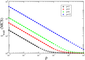
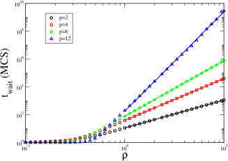
Figure 2: (Color online) (a) Temperature dependence and (b) density dependence of the average $t_{\text{wait}}$ in $d=2$ for $N=80$ particles. The solid lines are the power law fits.

We study the two-dimensional system with $N=80$ particles distributed on a triangular lattice of length $L$ and width $\sqrt{3}L/2$ with periodic boundary conditions for both axes. Fig. 2 (a) shows the temperature dependence of the average $t_{\text{wait}}$, in this case with the number of samples $10^{7}$ MCSp. The power law fits, all for $\rho\geq 1$, give $\langle t_{\text{wait}}\rangle\sim T^{-0.99(1)}$ with $r=1.0(1)$, for $p=2,4,6$ and 12. The density dependence is shown in Fig. 2 (b), $10^{6}$ MCSp are taken for $p=2,4,6$ and $10^{9}$ for $p=12$ at high densities. The power law fit for $p=2$ gives $\langle t_{\text{wait}}\rangle\sim\rho^{1.99(1)}$ with $r=-1.00(1)$, for $p=4$ gives $\langle t_{\text{wait}}\rangle\sim\rho^{3.00(1)}$ with $r=-1.00(1)$, for $p=6$ gives $\langle t_{\text{wait}}\rangle\sim\rho^{4.00(1)}$ with $r=-1.00(1)$, and for $p=12$ gives $\langle t_{\text{wait}}\rangle\sim\rho^{7.09(1)}$ with $r=-1.00(1)$. These results show excellent agreement with the asymptotic prediction $\langle t_{\text{wait}}\rangle\sim\>T\>\rho^{\frac{p+2}{2}}$ in Eq. (16).

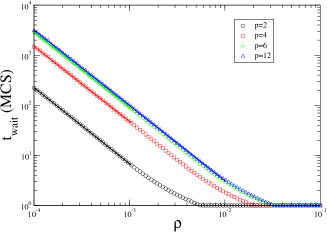
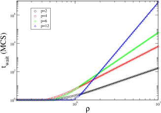
Figure 3: (Color online) (a) Temperature dependence and (b) density dependence of the average $t_{\text{wait}}$ for a 3-dimensional FCC system with $N=500$ particles. The solid lines are the power law fits.

We also study the 3-dimensional system with $N=500$ particles located on an FCC lattice with periodic boundary conditions for all directions. The temperature dependence and density dependence of the average $t_{\text{wait}}$ are shown in Fig. 3 (a) and Fig. 3 (b), respectively. The power law fits of the temperature dependence gives $\langle t_{\text{wait}}\rangle\sim T^{-1.49(1)}$ with $r=1.00(1)$, for $p=2,4,6$ and 12. The power law fit, all for $\rho\geq 1.1$, for the density dependence for $p=2$ gives $\langle t_{\text{wait}}\rangle\sim\rho^{1.98(1)}$ with $r=-1.00(1)$, for $p=4$ gives $\langle t_{\text{wait}}\rangle\sim\rho^{3.02(1)}$ with $r=-1.00(1)$, for $p=6$ gives $\langle t_{\text{wait}}\rangle\sim\rho^{4.01(1)}$ with $r=-1.00(1)$, and for $p=12$ gives $\langle t_{\text{wait}}\rangle\sim\rho^{6.96(1)}$ with $r=-1.00(1)$. The results agree with the asymptotic predictions $\langle t_{\text{wait}}\rangle\sim T^{-3/2}\rho^{(p+2)/2}$.

V Summary and Discussion

We studied the efficiency of the Rejection Free Monte Carlo (RFMC) method for systems having particles interacting through repulsive power-law potentials. The density and temperature dependence of the average waiting time has been predicted to be,

$$\langle t_{\text{wait}}\rangle\sim\frac{\rho^{\tfrac{p+2}{2}}}{T^{\tfrac{d}{2}}},$$ (20)

with the dimensionality of the system $d$, density $\rho$, and the temperature $T$, respectively. These theoretical results are valid asymptotically for large $\rho$ and/or low $T$. Monte Carlo simulations were performed and the results showed good agreement with the asymptotic prediction. This study shows how efficient the RFMC method is in low temperature or in high density regimes. Assume the wall-clock time per algorithmic step for the standard dynamic Monte Carlo algorithm is $t_{0}$, and the average wall-clock time per RFMC algorithmic step is $t_{1}$ (both of which are expected to be almost independent of $T$ and $\rho$). Because of the extra bookkeeping involved in programming the RFMC method, $t_{1}>t_{0}$. Nevertheless, the RFMC method will be more efficient (use less wall-clock time) whenever $t_{1}<t_{0}\langle t_{\rm wait}\rangle$. This inequality will always be satisfied for low enough $T$ or high enough density.

The RFMC method does not change the dynamic of the MC move associated with the underlying physical dynamics, and therefore makes possible the study of systems with a fixed physical dynamic. It is very important keeping the dynamics unchanged, since the change in the dynamics of the MC move can cause a strong influence in certain dynamic physical properties Park et al. (2004); Buendía et al. (2004); Gillespie (1976, 1977).

Although we studied a repulsive core power-law potential, we expect the equivalent behavior of the waiting time for more realistic potentials, as long as we work with the system at low temperatures and/or high densities. A further avenue of study, therefore, could be to calculate the efficiency of the RFMC method for more general potentials such as Lennard-Jones, or those derived from density functional theory. A related study could also be of the efficiency of the RFMC in the case of two or more types of particles. The actual implementation and utilization of the RFMC method in particle simulations can be attempted now that the ultimate behavior of the algorithmic efficiency has been determined.