Manin’s conjecture for a cubic surface with ${\mathbf{D}}_{5}$ singularity

Abstract

The Manin conjecture is established for a split singular cubic surface in ${\mathbb{P}^{3}}$, with singularity type ${\mathbf{D}}_{5}$.

1. Introduction

Let $S\subset{\mathbb{P}^{3}}$ be the cubic surface defined by

$$x_{3}x_{0}^{2}+x_{0}x_{2}^{2}+x_{2}x_{1}^{2}=0.$$ (1.1)

Then $S$ is a singular del Pezzo surface with a unique singularity $(0:0:0:1)$ of type ${\mathbf{D}}_{5}$ and three lines, each of which is defined over $\mathbb{Q}$.

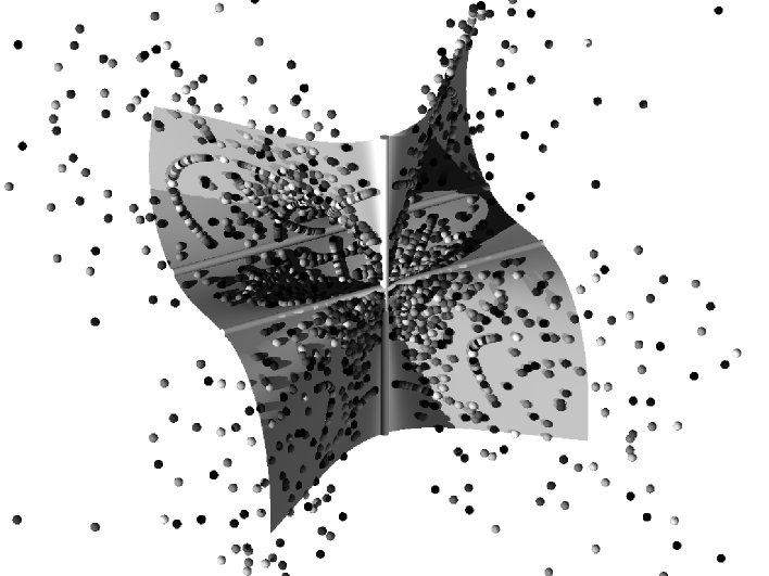
Figure 1. Points of height $\leqslant 100$ on the ${\mathbf{D}}_{5}$ cubic surface.

Let $U$ be the Zariski open subset formed by deleting the lines from $S$. Our principal object of study in this paper is the cardinality

$$N_{U,H}(B)=\#\{\mathbf{x}\in U(\mathbb{Q})\mid H(\mathbf{x})\leqslant B\},$$

for any $B\geqslant 1$. Here $H$ is the usual height on ${\mathbb{P}^{3}}$, in which $H(\mathbf{x})$ is defined as $\max\{|x_{0}|,\dots,|x_{3}|\}$, provided that the point $\mathbf{x}\in{\mathbb{P}^{3}}(\mathbb{Q})$ is represented by integral coordinates $(x_{0},\ldots,x_{3})$ that are relatively coprime. In Figure 1 we have plotted an affine model of $S$, together with all of the rational points of low height that it contains. The following is our principal result.

Theorem.

We have

$$N_{U,H}(B)=c_{S,H}B(\log B)^{6}+O\left(B(\log B)^{5}(\log\log B)\right),$$

where the leading constant is

$$c_{S,H}=\frac{1}{230400}\cdot\omega_{\infty}\cdot\prod_{p}\omega_{p}$$

with

$$\omega_{p} =\left(1-\frac{1}{p}\right)^{7}\left(1+\frac{7}{p}+\frac{1}{p^{2}}\right),$$

$$\omega_{\infty} =\int_{|x_{0}|,|x_{1}|,|x_{2}|,|x_{0}^{-2}(x_{0}x_{2}^{2}+x_{2}x_{1}^{2})|\leqslant 1,\ x_{2}\geqslant 0}x_{0}^{-2}\,\mathrm{d}x_{0}\,\mathrm{d}x_{1}\,\mathrm{d}x_{2}.$$

It is straightforward to check that the surface $S$ is neither toric nor an equivariant compactification of $\mathbb{G}_{\mathrm{a}}^{2}$. Thus this result does not follow from the work of Tschinkel and his collaborators [1, 7]. Our theorem confirms the conjecture of Manin [13] since the Picard group of the minimal desingularisation ${\widetilde{S}}$ of the split del Pezzo surface $S$ has rank $7$. Furthermore, the leading constant $c_{S,H}$ coincides with Peyre’s prediction [14]. To check this we begin by observing that

$$\alpha({\widetilde{S}})=\frac{\alpha(S_{0})}{\#W({\mathbf{D}}_{5})}=\frac{1/120}{1920}=\frac{1}{230400},$$

by [9, Theorem 4] and [12, Theorem 1.3], where $S_{0}$ is a split smooth cubic surface and $\#W({\mathbf{D}}_{5})$ is the order of the Weyl group of the root system ${\mathbf{D}}_{5}$. Next one easily verifies that the constant $\omega_{\infty}$ in the theorem is the real density, which is computed by writing $x_{3}$ as a function of $x_{0},x_{1},x_{2}$ and using the Leray form $x_{0}^{-2}\,\mathrm{d}x_{0}\,\mathrm{d}x_{1}\,\mathrm{d}x_{2}$. Finally, it is straightforward to compute the $p$-adic densities as being equal to $\omega_{p}$.

Our work is the latest in a sequence of attacks upon the Manin conjecture for del Pezzo surfaces, a comprehensive survey of which can be found in [5]. A number of authors have established the conjecture for the surface

$$x_{1}x_{2}x_{3}+x_{0}^{3}=0,$$

which has singularity type $3{\mathbf{A}}_{2}$. The sharpest unconditional result available is due to la Bretèche [2]. Furthermore, in joint work with la Bretèche [4], the authors have recently resolved the conjecture for the surface

$$x_{1}x_{2}^{2}+x_{2}x_{0}^{2}+x_{3}^{3}=0,$$

which has singularity type ${\mathbf{E}}_{6}$. Our main result signifies only the third example of a cubic surface for which the Manin conjecture has been resolved.

The proof of the theorem draws upon the expanding store of technical machinery that has been developed to study the growth rate of rational points on singular del Pezzo surfaces. In particular, we will take advantage of the estimates involving exponential sums that featured in [4]. In the latter setting these tools were required to get an asymptotic formula for the relevant counting function with error term of the shape $O(B^{1-\delta})$. However, in their present form, they are not even enough to establish an asymptotic formula in the ${\mathbf{D}}_{5}$ setting. Instead we will need to revisit the proofs of these results in order to sharpen the estimates to an extent that they can be used to establish the theorem. In addition to these refined estimates, we will often be in a position to abbreviate our argument by taking advantage of [10], where several useful auxiliary results are framed in a more general context.

In keeping with current thinking on the arithmetic of split del Pezzo surfaces, the proof of our theorem relies on passing to a universal torsor, which in the present setting is an open subset of the hypersurface

$$\eta_{2}\eta_{6}^{2}\alpha_{2}+\eta_{4}\eta_{5}^{2}\eta_{7}^{3}\eta_{8}+\eta_{3}\alpha_{1}^{2}=0,$$ (1.2)

embedded in $\mathbb{A}^{10}\cong\operatorname{Spec}\mathbb{Q}[\eta_{1},\ldots,\eta_{8},\alpha_{1},\alpha_{2}]$. Furthermore, as with most proofs of the Manin conjecture for singular del Pezzo surfaces of low degree, the shape of the cone of effective divisors of the corresponding minimal desingularisation plays an important role in our work. For the surfaces treated in [3], [4], [11], the fact that the effective cone is simplicial streamlines the proofs considerably. For the surface studied in [6], this was not the case, but it was nonetheless possible to exploit the fact that the dual of the effective cone is the difference of two simplicial cones. For the cubic surface (1.1), the dual of the effective cone is again the difference of two simplicial cones. However, we choose to ignore this fact and rely on a more general strategy instead.

Acknowledgements.

While working on this paper the first author was supported by EPSRC grant number EP/E053262/1. The second author was partially supported by a Feodor Lynen Research Fellowship of the Alexander von Humboldt Foundation. The authors are grateful to the referee for a number of useful comments that have improved the exposition of this paper.

2. Arithmetic functions and exponential sums

Define the multiplicative arithmetic functions

$$\phi^{*}(q)=\prod_{p\mid q}\left(1-\frac{1}{p}\right),\quad g(q)=\sum_{d\mid q}d^{-1/2},\quad h_{k}(q)=2^{\omega(q)}g(q)^{k},$$

for any $k\in\mathbb{Z}_{>0}$, where $\omega(q)$ denotes the number of distinct prime factors of $q$. These functions will feature quite heavily in our work and we will need to know the average order of the latter.

Lemma 1.

For any $k\in\mathbb{Z}_{>0}$ we have

$$\sum_{q\leqslant Q}h_{k}(q)\ll_{k}Q\log Q.$$

Proof.

Let $k\in\mathbb{Z}_{>0}$ be given and let $\varepsilon>0$. Then we have

$$\sum_{q\leqslant Q}h_{k}(q) =\sum_{q\leqslant Q}2^{\omega(q)}\sum_{d_{1},\ldots,d_{k}\mid q}(d_{1}\cdots d_{k})^{-1/2}$$

$$\ll_{\varepsilon}\sum_{d_{1},\ldots,d_{k}=1}^{\infty}(d_{1}\cdots d_{k})^{\varepsilon-1/2}\sum_{u\leqslant Q/[d_{1},\ldots,d_{k}]}2^{\omega(u)}$$

$$\ll_{\varepsilon}Q\log Q\sum_{d_{1},\ldots,d_{k}=1}^{\infty}\frac{(d_{1}\cdots d_{k})^{\varepsilon-1/2}}{[d_{1},\ldots,d_{k}]},$$

where $[a,b]$ denotes the least common multiple of $a,b\in\mathbb{Z}_{>0}$. We easily check that the final sum is absolutely convergent by considering the corresponding Euler product, which has local factors of the shape $1+O_{\varepsilon}(p^{\varepsilon-3/2})$. ∎

Given integers $a,b,q$, with $q>0$, we will be led to consider the quadratic exponential sum

$$S_{q}(a,b)=\sum_{v=1}^{q}e_{q}(av^{2}+bv).$$ (2.1)

Our study of this should be compared with the corresponding sum studied in [4, Eq. (3.1)], involving instead a cubic phase $av^{3}+bv^{2}$. In [4, Lemma 4] an upper bound of the shape $O_{\varepsilon}(\gcd(q,b)q^{1/2+\varepsilon})$ is established for the cubic sum. The following result shows that we can do better in the quadratic setting.

Lemma 2.

For any $a,b\in\mathbb{Z}$ with $\gcd(q,a,b)=1$, we have

$$S_{q}(a,b)\ll\gcd(q,a)^{1/2}q^{1/2}.$$

Proof.

Writing $w=v+x$ in the second step, we find that

$$\begin{split}|S_{q}(a,b)|^{2}&=\sum_{v,w=1}^{q}e_{q}(a(v^{2}-w^{2})+b(v-w))\\ &=\sum_{v,x=1}^{q}e_{q}(-a(2vx+x^{2})-bx)\\ &=\sum_{x=1}^{q}e_{q}(-ax^{2}-bx)\sum_{v=1}^{q}e_{q}(-2avx)\end{split}$$

The inner sum is $q$ if $q\mid 2ax$ and $0$ otherwise. Let $h=\gcd(a,q)$ and write $q=hq^{\prime}$, $a=ha^{\prime}$ with ${\gcd(a^{\prime},q^{\prime})=1}$. Then

$$|S_{q}(a,b)|^{2}=q\sum_{\begin{subarray}{c}x=1\\ q^{\prime}\mid 2x\end{subarray}}^{q}e_{q}(-ax^{2}-bx)\leqslant 2qh,$$

and the result follows. ∎

Our next results concern the function $\psi(t)=\{t\}-1/2$, where $\{t\}$ is the fractional part of $t\in\mathbb{R}$. The following estimate improves upon [3, Lemma 5].

Lemma 3.

For any $t\in\mathbb{R}$, $b\in\mathbb{Z}$, $q\in\mathbb{Z}_{>0}$ with ${\gcd(b,q)=1}$, we have

$$\sum_{\begin{subarray}{c}x=1\\ {\gcd(x,q)=1}\end{subarray}}^{q}\psi\left(\frac{t-bx^{2}}{q}\right)\ll h_{1}(q)\log(q+1)q^{1/2}.$$

Proof.

Let $S(q)$ denote the sum that is to be estimated. By Möbius inversion it follows that

$$\begin{split}S(q)&=\sum_{n\mid q}\mu(n)\sum_{0\leqslant x^{\prime}<q/n}\psi\left(\frac{t/n-bnx^{\prime 2}}{q/n}\right)\\ &=\sum_{\begin{subarray}{c}n\mid q\\ m=\gcd(n,q/n)\end{subarray}}\mu(n)m\sum_{0\leqslant x^{\prime}<\frac{q}{mn}}\psi\left(\frac{t/(mn)-bnx^{\prime 2}/m}{q/(mn)}\right).\end{split}$$

We claim that

$$\sum_{0\leqslant x<q}\psi\left(\frac{t-bx^{2}}{q}\right)\ll g(q)\log(q+1)q^{1/2},$$ (2.2)

for any $t\in\mathbb{R}$, $b\in\mathbb{Z}$ and $q\in\mathbb{Z}_{>0}$ with ${\gcd(b,q)=1}$. Under this assumption, it therefore follows that

$$\begin{split}S(q)&\ll\sum_{\begin{subarray}{c}n\mid q\\ m=\gcd(n,q/n)\end{subarray}}|\mu(n)|mg(q)\log(q+1)(q/(mn))^{1/2}\\ &=g(q)\log(q+1)q^{1/2}\sum_{n\mid q}\frac{|\mu(n)|\gcd(n,q/n)^{1/2}}{n^{1/2}}\\ &\ll 2^{\omega(q)}g(q)\log(q+1)q^{1/2}.\end{split}$$

This is satisfactory for the lemma, since $h_{1}(q)=2^{\omega(q)}g(q)$.

To establish (2.2) we follow the proof of [3, Lemma 4], finding that

$$\sum_{0\leqslant x<q}\psi\left(\frac{t-bx^{2}}{q}\right)\ll 1+\sum_{m\mid q}\sum_{\begin{subarray}{c}1\leqslant\ell^{\prime}<q/m\\ {\gcd(\ell^{\prime},q/m)=1}\end{subarray}}\frac{|T(q,m,\ell^{\prime})|}{q\|\ell^{\prime}m/q\|},$$

where

$$T(q,m,\ell^{\prime})=\sum_{0\leqslant x<q}e_{q/m}(\ell^{\prime}bx^{2}).$$

Rather than applying Weyl’s inequality as in [3, Lemma 4], we simply break into $m$ residue classes modulo $q/m$ and apply Lemma 2 to deduce that

$$T(q,m,\ell^{\prime})\ll m(q/m)^{1/2}=(mq)^{1/2}.$$

Now

$$\sum_{1\leqslant\ell^{\prime}<r}\|\ell^{\prime}/r\|^{-1}\ll r\sum_{1\leqslant\ell^{\prime}<r}\ell^{\prime-1}\ll r\log(r+1),$$

for any $r\in\mathbb{Z}_{>0}$. Hence

$$\begin{split}\sum_{0\leqslant x<q}\psi\left(\frac{t-bx^{2}}{q}\right)&\ll 1+\log(q+1)q^{1/2}\sum_{m\mid q}m^{-1/2}\\ &\ll g(q)\log(q+1)q^{1/2},\end{split}$$

which thereby concludes the proof of (2.2). ∎

For positive integers $a,b$, we define the function

$$f_{a,b}(n)=\begin{cases}\phi^{*}(n)/\phi^{*}(\gcd(n,a)),&\mbox{if ${\gcd(n,b)=1}$},\\ 0,&\mbox{if ${\gcd(n,b)>1}$}.\end{cases}$$ (2.3)

We combine Lemma 3 with the proof of [6, Lemma 1] to obtain the following result.

Lemma 4.

Let $0\leqslant t_{1}<t_{2}$ and ${\gcd(\alpha,q)=1}$. We have

$$\sum_{\begin{subarray}{c}1\leqslant\varrho\leqslant q\\ {\gcd(\varrho,q)=1}\end{subarray}}\sum_{\begin{subarray}{c}t_{1}<n\leqslant t_{2}\\ {n}\equiv{\alpha\varrho^{2}}\ (\mathrm{mod}\ {q})\end{subarray}}f_{a,b}(n)=(t_{2}-t_{1})\cdot\phi^{*}(bq)\prod_{p\nmid abq}\left(1-\frac{1}{p^{2}}\right)\\ +O\left(2^{\omega(b)}\log(t_{2}+2)h_{1}(q)\log(q+1)q^{1/2}\right).$$

Proof.

In the proof of [6, Lemma 1],

$$\Sigma=\sum_{\begin{subarray}{c}d^{-1}t_{1}<m\leqslant d^{-1}t_{2}\\ {md}\equiv{\alpha\varrho^{2}}\ (\mathrm{mod}\ {q})\end{subarray}}1$$

is estimated as $(t_{2}-t_{1})/(dq)+O(1)$, for given $d$ coprime to $q$. Using [4, Lemma 7], we make this precise as

$$\Sigma=\frac{t_{2}-t_{1}}{dq}+\psi\left(\frac{d^{-1}t_{1}-\overline{d}\alpha\varrho^{2}}{q}\right)-\psi\left(\frac{d^{-1}t_{2}-\overline{d}\alpha\varrho^{2}}{q}\right),$$

where $\overline{d}$ is chosen such that ${d\overline{d}}\equiv{1}\ (\mathrm{mod}\ {q})$. Our task is to compute

$$\sum_{\begin{subarray}{c}1\leqslant\varrho\leqslant q\\ {\gcd(\varrho,q)=1}\end{subarray}}\sum_{\begin{subarray}{c}1\leqslant d\leqslant t_{2}\\ {\gcd(d,q)=1}\end{subarray}}(f_{a,b}*\mu)(d)\Sigma.$$

For the main term, we may extend the summation over $d$ to all positive integers, since

$$\sum_{1\leqslant\varrho\leqslant q}\frac{t_{2}-t_{1}}{q}\sum_{\begin{subarray}{c}d>t_{2}\\ {\gcd(d,q)=1}\end{subarray}}\frac{(f_{a,b}*\mu)(d)}{d}\ll t_{2}\sum_{d>t_{2}}\frac{\gcd(b,d)|\mu(d)|}{d^{2}}\ll 2^{\omega(b)}.$$

As in [6, Lemma 1], we see that the sum over $d\in\mathbb{Z}_{>0}$ is $c_{0}(t_{2}-t_{1})/q$, with

$$c_{0}=\prod_{\begin{subarray}{c}p\mid b\\ p\nmid q\end{subarray}}\left(1-\frac{1}{p}\right)\prod_{p\nmid abq}\left(1-\frac{1}{p^{2}}\right).$$

Summing this over $\varrho$, we get $c_{0}\phi^{*}(q)(t_{2}-t_{1})$. It is easy to see that $c_{0}\phi^{*}(q)$ agrees with the leading constant in the statement of the lemma.

For the error term, we exchange the summations over $d$ and $\varrho$. Applying Lemma 3, we obtain the contribution

$$\begin{split}&\ll F(q)\sum_{\begin{subarray}{c}1\leqslant d\leqslant t_{2}\\ {\gcd(d,q)=1}\end{subarray}}|(f_{a,b}*\mu)(d)|\ll 2^{\omega(b)}\log(t_{2}+2)F(q),\end{split}$$

with $F(q)=h_{1}(q)\log(q+1)q^{1/2}$. This completes the proof of the lemma. ∎

Given $b,c,q\in\mathbb{Z}$ such that $q>0$ and a real-valued function $f$ defined on an interval $I\subset\mathbb{R}$, let

$$S_{I}(f,q)=\sum_{x\in\mathbb{Z}\cap I}\sum_{\begin{subarray}{c}y=1\\ {y^{2}}\equiv{bx}\ (\mathrm{mod}\ {q})\\ {\gcd(y,q)=1}\end{subarray}}^{q}\psi\left(\frac{f(x)-cy}{q}\right).$$

It is interesting to compare this sum with the sort of sums that featured in our corresponding investigation of the ${\mathbf{E}}_{6}$ cubic surface. The sole difference between [4, Eq. (4.1)] and $S_{I}(f,q)$ is that the argument involves $(f(x)-cxy)/q$, rather than $(f(x)-cy)/q$.

We will be interested in studying $S_{I}(f,q)$ when $f\in C^{1}(I;\lambda_{0})$. Here, if $I=[t_{1},t_{2}]$ and $\lambda_{0}\geqslant 1$, then $C^{1}(I;\lambda_{0})$ is defined to be the set of real-valued differentiable functions $f$, such that $f^{\prime}$ is monotonic and of constant sign on $(t_{1},t_{2})$, with $|f(t_{2})-f(t_{1})|+1\leqslant\lambda_{0}$. It will be convenient to define

$$\mathfrak{m}(I)=\operatorname{meas}(I)+2.$$

We will need a version of [4, Lemma 10], in which the factor $q^{\varepsilon}\mathfrak{m}(I)^{\varepsilon}$ is made more explicit. This is achieved in the following result.

Lemma 5.

Let $X=q\mathfrak{m}(I)$. Assume ${\gcd(bc,q)=1}$ and $f\in C^{1}(I;\lambda_{0})$. For any $\varepsilon>0$, we have

$$S_{I}(f,q)\ll\left(h_{2}(q)q^{1/2}+\tau(q)^{2}\frac{\mathfrak{m}(I)}{q}+\frac{h_{1}(q)}{\log X}\frac{\lambda_{0}^{1/2}\mathfrak{m}(I)^{1/2}}{q^{1/4}}\right)(\log X)^{2},$$

where $\tau(n)=\sum_{d|n}1$ is the divisor function.

In comparing this with [4, Lemma 10], one sees that the first and third term in both results share the same approximate order of magnitude. However, the middle term is improved from $1/q^{1/3}$ to $1/q$. This saving is crucial in our work. It arises from the fact that the current set-up leads us to estimate the quadratic exponential sums (2.1) with $a=0$, rather than the corresponding cubic sums with phase $av^{3}+bv^{2}$ and $b=0$. In the former case we are dealing with linear exponential sums, for which we have very good control, and in the latter case we only have the bound $O_{\varepsilon}(q^{2/3+\varepsilon})$ available.

Proof of Lemma 5.

Let $\eta(\alpha;q)=\#\{1\leqslant n\leqslant q\mid{n^{2}}\equiv{\alpha}\ (\mathrm{mod}\ {q})\}$. Replacing the bound $\eta(\alpha;q)\ll_{\varepsilon}q^{\varepsilon}$ by $\eta(\alpha;q)\leqslant 2^{\omega(q)+1}$ in the application of Vaaler’s trigonometric formula in the proof of [4, Lemma 10], we obtain

$$S_{I}(f,q)\ll\frac{2^{\omega(q)}\mathfrak{m}(I)}{H}+\sum_{h=1}^{H}\frac{1}{h}|T_{I}(f,q;h)|$$

for any $H\geqslant 1$, where

$$T_{I}(f,q;h)=\sum_{x\in\mathbb{Z}\cap I}\sum_{\begin{subarray}{c}y=1\\ {y^{2}}\equiv{bx}\ (\mathrm{mod}\ {q})\\ {\gcd(y,q)=1}\end{subarray}}^{q}e_{q}(hf(x)-chy).$$

As in [4, Lemma 10], we rewrite this as

$$T_{I}(f,q;h)=\frac{1}{q}\sum_{k=1}^{q}A_{I}(q;-k,h,f)B(q;h,k),$$

with

$$A_{I}(q;-k,h,f)=\sum_{x\in\mathbb{Z}\cap I}e_{q}(-kx+hf(x))$$

and

$$B(q;h,k)=\sum_{u=1}^{q}\sum_{\begin{subarray}{c}v=1\\ {v^{2}}\equiv{bu}\ (\mathrm{mod}\ {q})\\ {\gcd(v,q)=1}\end{subarray}}^{q}e_{q}(ku-chv)=\sum_{\begin{subarray}{c}v=1\\ {\gcd(v,q)=1}\end{subarray}}^{q}e_{q}(\overline{b}kv^{2}-chv),$$

where $\overline{b}$ is the multiplicative inverse of $b$ modulo $q$. Since $\gcd(q,\overline{b}k,ch)=\gcd(q,k,h)$, we have (with $h=dh^{\prime},\ k=dk^{\prime},\ q=dq^{\prime}$)

$$T_{I}(f,q;h)=\sum_{d|h,q}\frac{1}{dq^{\prime}}\sum_{\begin{subarray}{c}-q^{\prime}/2<k^{\prime}\leqslant q^{\prime}/2\\ \gcd(k^{\prime},h^{\prime},q^{\prime})=1\end{subarray}}A_{I}(q^{\prime};-k^{\prime},h^{\prime},f)B(dq^{\prime};dh^{\prime},dk^{\prime}).$$

Write each $v$ modulo $q$ uniquely as $v=y+q^{\prime}z$ with $1\leqslant y\leqslant q^{\prime}$ and $1\leqslant z\leqslant d$. Then

$$B(dq^{\prime};dh^{\prime},dk^{\prime})=\sum_{y=1}^{q^{\prime}}\sum_{\begin{subarray}{c}z=1\\ {\gcd(y+q^{\prime}z,dq^{\prime})=1}\end{subarray}}^{d}e_{q^{\prime}}(\overline{b}k^{\prime}y^{2}-ch^{\prime}y)=f(d,q^{\prime})B(q^{\prime};h^{\prime},k^{\prime})$$

with $f(d,q^{\prime})\leqslant d$, just as in [4, Lemma 10]. Therefore,

$$T_{I}(f,q;h)\ll\sum_{d\mid h,q}\frac{1}{q^{\prime}}\sum_{\begin{subarray}{c}-q^{\prime}/2<k^{\prime}\leqslant q^{\prime}/2\\ \gcd(k^{\prime},h^{\prime},q^{\prime})=1\end{subarray}}|A_{I}(q^{\prime};-k^{\prime},h^{\prime},f)||B(q^{\prime};h^{\prime},k^{\prime})|.$$

For the contribution from the case $k^{\prime}=0$, note that ${\gcd(h^{\prime},q^{\prime})=1}$. We have $A_{I}(q^{\prime};0,h^{\prime},f)\ll\mathfrak{m}(I)$ trivially, and

$$B(q^{\prime};h^{\prime},0)=\sum_{\begin{subarray}{c}v=1\\ {\gcd(v,q^{\prime})=1}\end{subarray}}^{q^{\prime}}e_{q^{\prime}}(-ch^{\prime}v)=\sum_{d\mid q^{\prime}}\mu(d)\sum_{v=1}^{q^{\prime}/d}e_{q^{\prime}/d}(-ch^{\prime}v).$$

The inner sum is $q^{\prime}/d$ if $(q^{\prime}/d)\mid ch^{\prime}$ (which is possible only in the case $q^{\prime}/d=1$ since $\gcd(q,c)={\gcd(q^{\prime},h^{\prime})=1}$) and $0$ otherwise. Thus $B(q^{\prime};h^{\prime},0)=\mu(q^{\prime})$, whence the total contribution to $T_{I}(f,q;h)$ from the case $k^{\prime}=0$ is

$$\ll\sum_{d\mid h,q}\frac{1}{q^{\prime}}\mathfrak{m}(I)|\mu(q^{\prime})|\ll\frac{\mathfrak{m}(I)}{q}\sigma(\gcd(h,q)),$$

where $\sigma(n)=\sum_{d\mid n}d$ is the sum of divisors function.

For the total contribution to $T_{I}(f,q;h)$ from the case $k^{\prime}\neq 0$, we note that

$$A_{I}(q^{\prime};-k^{\prime},h^{\prime},f)\ll\frac{1}{|k^{\prime}|}(q^{\prime}+h^{\prime}\lambda_{0})=\frac{q^{\prime}}{|k^{\prime}|}(1+h\lambda_{0}/q),$$

by [4, Lemma 5] for $f\in C^{1}(I;\lambda_{0})$. Also

$$B(q^{\prime};h^{\prime},k^{\prime})=\sum_{\begin{subarray}{c}v=1\\ {\gcd(v,q^{\prime})=1}\end{subarray}}^{q^{\prime}}e_{q^{\prime}}(\overline{b}k^{\prime}v^{2}-ch^{\prime}v)=\sum_{e\mid q^{\prime}}\mu(e)\sum_{v=1}^{q^{\prime\prime}}e_{q^{\prime\prime}}(\overline{b}k^{\prime}ev^{2}-ch^{\prime}v),$$

where $q^{\prime}=eq^{\prime\prime}$. By Lemma 2,

$$\begin{split}|B(q^{\prime};h^{\prime},k^{\prime})|&\ll\sum_{e\mid q^{\prime}}|\mu(e)|q^{\prime\prime 1/2}\gcd(q^{\prime\prime},\overline{b}k^{\prime}e)^{1/2}\\ &\leqslant\sum_{e\mid q^{\prime}}|\mu(e)|\frac{q^{\prime 1/2}}{e^{1/2}}\gcd(q^{\prime},k^{\prime})^{1/2}\gcd(q^{\prime\prime},e)^{1/2}\\ &\leqslant 2^{\omega(q^{\prime})}\gcd(q^{\prime},k^{\prime})^{1/2}q^{\prime 1/2}.\end{split}$$

The contribution from the case $k^{\prime}\neq 0$ is therefore

$$\begin{split}&\ll\sum_{d\mid h,q}\frac{d}{q}\sum_{\begin{subarray}{c}1\leqslant k^{\prime}\leqslant q^{\prime}/2\\ \gcd(k^{\prime},h^{\prime},q^{\prime})=1\end{subarray}}\frac{q^{\prime}}{k^{\prime}}(1+h\lambda_{0}/q)2^{\omega(q^{\prime})}\gcd(q^{\prime},k^{\prime})^{1/2}q^{\prime 1/2}\\ &\ll(1+h\lambda_{0}/q)2^{\omega(q)}q^{1/2}\sum_{d\mid h,q}\frac{1}{d^{1/2}}\sum_{k^{\prime}\leqslant q^{\prime}/2}\frac{\gcd(q^{\prime},k^{\prime})^{1/2}}{k^{\prime}}\\ &\ll(1+h\lambda_{0}/q)h_{2}(q)\log(q+1)q^{1/2}.\end{split}$$

Plugging the contribution from $k^{\prime}=0$ and $k^{\prime}\neq 0$ to $T_{I}(f,q;h)$ into $S_{I}(f,q)$, we deduce, for any $H\geqslant 1$, that $S_{I}(f,q)$ is

$$\ll{}\frac{2^{\omega(q)}\mathfrak{m}(I)}{H}+\sum_{h=1}^{H}\frac{1}{h}\left((1+h\lambda_{0}/q)h_{2}(q)\log(q+1)q^{1/2}+\frac{\mathfrak{m}(I)}{q}\sigma(\gcd(h,q))\right).$$

Observing that

$$\sum_{h\leqslant H}\frac{\sigma(\gcd(h,q))}{h}=\sum_{d\mid q}\sigma(d)\sum_{\begin{subarray}{c}h\leqslant H\\ d\mid h\end{subarray}}\frac{1}{h}\ll(\log H)\sum_{d\mid q}\frac{\sigma(d)}{d}\ll(\log H)\tau(q)^{2},$$

we therefore deduce that

$$S_{I}(f,q)\ll\frac{2^{\omega(q)}\mathfrak{m}(I)}{H}+\frac{\tau(q)^{2}\mathfrak{m}(I)(\log H)}{q}+\log(q+1)h_{2}(q)q^{1/2}(\log H)\\ +\log(q+1)h_{2}(q)\lambda_{0}H/q^{1/2}.$$

Let

$$H=\frac{q^{1/4}\mathfrak{m}(I)^{1/2}}{\lambda_{0}^{1/2}\log(q+1)^{1/2}g(q)}.$$

If $H\geqslant 1$, we may use this $H$ in the estimate above, together with $q+1\leqslant X$, in order to obtain the lemma. If $H<1$, so that $q^{1/4}\mathfrak{m}(I)^{1/2}<\lambda_{0}^{1/2}(\log q)^{1/2}g(q)$, we deduce from the trivial estimate $S_{I}(f,q)\ll 2^{\omega(q)}\mathfrak{m}(I)$ that the lemma holds in this case too. ∎

3. The universal torsor

Let $S$ be the ${\mathbf{D}}_{5}$ cubic surface (1.1), let $U\subset S$ be the open subset formed by deleting the lines from $S$ and let ${\widetilde{S}}$ be the minimal desingularisation of $S$. In this section we will establish an explicit bijection between $U(\mathbb{Q})$ and the integral points on the universal torsor above ${\widetilde{S}}$, subject to a number of coprimality conditions. For this we will follow the strategy explained in [11].

To establish the bijection we will introduce new variables $\eta_{1},\ldots,\eta_{8}$ and $\alpha_{1},\alpha_{2}$. It will be convenient to henceforth write

$$\boldsymbol{\eta}=(\eta_{1},\dots,\eta_{6}),\quad\boldsymbol{\eta}^{\prime}=(\eta_{1},\dots,\eta_{8}),\quad\boldsymbol{\alpha}=(\alpha_{1},\alpha_{2})$$

and

$$\boldsymbol{\eta}^{({k_{1}},{k_{2}},{k_{3}},{k_{4}},{k_{5}},{k_{6}})}=\prod_{i=1}^{6}\eta_{i}^{k_{i}},$$

for any $(k_{1},\dots,k_{6})\in\mathbb{Q}^{6}$.

Let us recall some information concerning the geometry of $S$ from [8, Section 8]. Blowing up the singularity $(0:0:0:1)$ on $S$ results in the exceptional divisors $E_{1},\dots,E_{5}$ in a ${\mathbf{D}}_{5}$-configuration on the minimal desingularisation $\pi:{\widetilde{S}}\to S$. Let $E_{6},E_{7},E_{8}$ resp. $A_{1},A_{2}$ on ${\widetilde{S}}$ be the strict transforms under $\pi$ of the three lines $E_{6}^{\prime\prime}=\{x_{0}=x_{1}=0\}$, $E_{7}^{\prime\prime}=\{x_{0}=x_{2}=0\}$, $E_{8}^{\prime\prime}=\{x_{2}=x_{3}=0\}$ resp. the curves $A_{1}^{\prime\prime}=\{x_{1}=x_{0}x_{3}+x_{2}^{2}=0\}$ and $A_{2}^{\prime\prime}=\{x_{3}=x_{0}x_{2}+x_{1}^{2}=0\}$ on $S$. The extended Dynkin diagram in Figure 2 is the dual graph of the configuration of the curves $E_{1},\dots,E_{8},A_{1},A_{2}$ on ${\widetilde{S}}$.

Figure 2. Configuration of curves on ${\widetilde{S}}$.

By [8, Section 8], non-zero global sections $\eta_{1},\dots,\eta_{8},\alpha_{1},\alpha_{2}$ corresponding to $E_{1},\dots,E_{8},A_{1},A_{2}$ form a generating set of the Cox ring of ${\widetilde{S}}$. The ideal of relations in $\operatorname{Cox}({\widetilde{S}})$ is generated by $\eta_{2}\eta_{6}^{2}\alpha_{2}+\eta_{4}\eta_{5}^{2}\eta_{7}^{3}\eta_{8}+\eta_{3}\alpha_{1}^{2}$. We express the sections $\pi^{*}(x_{i})$, for $0\leqslant i\leqslant 3$, of the anticanonical class $-K_{\widetilde{S}}$ in terms of the generators of $\operatorname{Cox}({\widetilde{S}})$ as follows:

$$(\pi^{*}(x_{0}),\dots,\pi^{*}(x_{3}))=(\boldsymbol{\eta}^{({4},{3},{2},{3},{2},{2})}\eta_{7},\boldsymbol{\eta}^{({3},{2},{2},{2},{1},{1})}\alpha_{1},\boldsymbol{\eta}^{({2},{1},{1},{2},{2},{0})}\eta_{7}^{2}\eta_{8},\eta_{8}\alpha_{2}).$$

The general strategy of [11] suggests that $U(\mathbb{Q})$ should be parametrised by certain integral points on the variety $\operatorname{Spec}(\operatorname{Cox}({\widetilde{S}}))$. This is confirmed in the the following result.

Lemma 6.

We have

$$N_{U,H}(B)=\#\mathcal{T}(B),$$

where $\mathcal{T}(B)$ is the set of $(\boldsymbol{\eta}^{\prime},\boldsymbol{\alpha})\in\mathbb{Z}_{>0}^{7}\times\mathbb{Z}_{\neq 0}\times\mathbb{Z}^{2}$ such that (1.2) holds, with

$$\max\{|\boldsymbol{\eta}^{({4},{3},{2},{3},{2},{2})}\eta_{7}|,|\boldsymbol{\eta}^{({3},{2},{2},{2},{1},{1})}\alpha_{1}|,|\boldsymbol{\eta}^{({2},{1},{1},{2},{2},{0})}\eta_{7}^{2}\eta_{8}|,|\eta_{8}\alpha_{2}|\}\leqslant B$$ (3.1)

and

$${\gcd(\alpha_{2},\eta_{1}\eta_{2}\eta_{7})=1},$$ (3.2)

$${\gcd(\alpha_{1},\eta_{1}\eta_{4}\eta_{5})=1},$$ (3.3)

$${\gcd(\eta_{8},\eta_{1}\eta_{2}\eta_{3}\eta_{4}\eta_{5}\eta_{6})=1},$$ (3.4)

$${\gcd(\eta_{7},\eta_{1}\eta_{2}\eta_{3}\eta_{4}\eta_{6})=1},$$ (3.5)

coprimality between $$\eta_{1},\dots,\eta_{6}$$ as in Figure 2. (3.6)

The coprimality conditions in (3.6) are achieved by taking $\eta_{i}$ and $\eta_{j}$ to be coprime if and only if the divisors $E_{i}$ and $E_{j}$ are not adjacent in the diagram. The reader is invited to consider the correspondence between

• the variables of the parametrisation and the generators of $\operatorname{Cox}({\widetilde{S}})$,

• the torsor equation (1.2) and the relation in $\operatorname{Cox}({\widetilde{S}})$,

• the height conditions (3.1) and the expressions of $\pi^{*}(x_{i})$ in terms of the generators of $\operatorname{Cox}({\widetilde{S}})$,

• the coprimality conditions (3.2)– (3.6) and the configuration of the curves associated to the generators of $\operatorname{Cox}({\widetilde{S}})$ encoded in Figure 2.

The proof of Lemma 6 is elementary, but modelled according to the geometry of $S$. The following additional geometric information is relevant. Contracting $E_{6},E_{2},E_{1},E_{3},E_{7},E_{5}$ in this order leads to a map $\phi_{1}:{\widetilde{S}}\to{\mathbb{P}^{2}}$ that is the blow-up of six points in the projective plane. We may choose $\phi_{1}(E_{4}),\phi_{1}(A_{1}),\phi_{1}(E_{8})$ as the coordinate lines in ${\mathbb{P}^{2}}=\{(\eta_{4}^{\prime}:\alpha_{1}^{\prime}:\eta_{8}^{\prime})\}$. Then $\phi_{1}(A_{2})$ is the quadric $\eta_{4}^{\prime}\eta_{8}^{\prime}+\alpha_{1}^{\prime 2}=0$. The morphisms $\phi_{1},\pi$ and the projection

$$\begin{array}[h]{cccc}\phi_{2}:&S&\dashrightarrow&{\mathbb{P}^{2}},\\ &\mathbf{x}&\mapsto&(x_{0}:x_{1}:x_{2})\end{array}$$

from the singularity $(0:0:0:1)$, form a commutative diagram of rational maps between ${\widetilde{S}},S$ and ${\mathbb{P}^{2}}$. The inverse map of $\phi_{2}$ is

$$\begin{array}[h]{cccc}\phi_{3}:&{\mathbb{P}^{2}}&\dashrightarrow&S,\\ &(\eta_{4}^{\prime}:\alpha_{1}^{\prime}:\eta_{8}^{\prime})&\mapsto&(\eta_{4}^{\prime 3}:\eta_{4}^{\prime 2}\alpha_{1}^{\prime}:\eta_{4}^{\prime 2}\eta_{8}^{\prime}:\eta_{8}^{\prime}\alpha_{2}^{\prime})\end{array}$$

where $\alpha_{2}^{\prime}=-\eta_{4}^{\prime}\eta_{8}^{\prime}-\alpha_{1}^{\prime 2}$. The maps $\phi_{2},\phi_{3}$ give a bijection between the complement $U$ of the lines on $S$ and $\{(\eta_{4}^{\prime}:\alpha_{1}^{\prime}:\eta_{8}^{\prime})\in{\mathbb{P}^{2}}\mid\eta_{4}^{\prime},\eta_{8}^{\prime}\neq 0\}$, and furthermore, induces a bijection between $U(\mathbb{Q})$ and the integral points

$$\{(\eta_{4},\alpha_{1},\eta_{8},\alpha_{2})\in\mathbb{Z}_{>0}\times\mathbb{Z}\times\mathbb{Z}_{\neq 0}\times\mathbb{Z}\mid\gcd(\eta_{4},\alpha_{1},\alpha_{2})=1,\ \alpha_{2}+\eta_{4}\eta_{8}+\alpha_{1}^{2}=0\}.$$

Motivated by the way the curves $E_{5},E_{7},E_{3},E_{1},E_{2},E_{6}$ occur in $\phi_{1}$ as the blow-ups of intersection points of $\phi_{1}(E_{4}),\phi_{1}(E_{8}),\phi_{1}(A_{1}),\phi_{1}(A_{2})$, one introduces the following further variables

$$\begin{array}[h]{lll}\eta_{5}=\gcd(\eta_{4},\eta_{8}),&\eta_{7}=\gcd(\eta_{5},\eta_{8}),&\eta_{3}=\gcd(\eta_{4},\alpha_{1},\alpha_{2}),\\ \eta_{1}=\gcd(\eta_{3},\eta_{4},\alpha_{2}),&\eta_{2}=\gcd(\eta_{1},\alpha_{2})&\eta_{6}=\gcd(\eta_{2},\alpha_{2}).\end{array}$$

Although we omit the details here, it is now straightforward to derive the bijection described in the statement of Lemma 6 using elementary number theory.

In analysing the height conditions apparent in (3.1) we will meet a number of real-valued functions, whose size it will be crucial to understand. We begin with the observation that (3.1) is equivalent to $h(\boldsymbol{\eta}^{\prime},\alpha_{1};B)\leqslant 1$, where

$$h(\boldsymbol{\eta}^{\prime},\alpha_{1};B)=B^{-1}\max\left\{\begin{aligned} &|\boldsymbol{\eta}^{({4},{3},{2},{3},{2},{2})}\eta_{7}|,|\boldsymbol{\eta}^{({3},{2},{2},{2},{1},{1})}\alpha_{1}|,\\ &|\boldsymbol{\eta}^{({2},{1},{1},{2},{2},{0})}\eta_{7}^{2}\eta_{8}|,\left|\frac{\eta_{4}\eta_{5}^{2}\eta_{7}^{3}\eta_{8}^{2}+\eta_{3}\eta_{8}\alpha_{1}^{2}}{\eta_{2}\eta_{6}^{2}}\right|\end{aligned}\right\}.$$

In what follows we will need to work with the regions

$$\begin{split}\mathcal{R}(B)&=\{(\boldsymbol{\eta}^{\prime},\alpha_{1})\in\mathbb{R}^{9}\,\Big{|}\,\eta_{1},\dots,\eta_{7},|\eta_{8}|\geqslant 1,\ h(\boldsymbol{\eta}^{\prime},\alpha_{1};B)\leqslant 1\},\\ \mathcal{R}^{\prime}_{1}(B)&=\{\boldsymbol{\eta}\in\mathbb{R}^{6}\mid\eta_{1},\dots,\eta_{6}\geqslant 1,\ \boldsymbol{\eta}^{({4},{3},{2},{3},{2},{2})}\leqslant B,\ \boldsymbol{\eta}^{({6},{5},{3},{4},{2},{4})}\geqslant B\},\\ \mathcal{R}^{\prime}_{2}(\boldsymbol{\eta};B)&=\{(\eta_{7},\eta_{8},\alpha_{1})\in\mathbb{R}^{3}\mid\eta_{7}\geqslant 0,\ h(\boldsymbol{\eta}^{\prime},\alpha_{1};B)\leqslant 1\},\\ \mathcal{R}^{\prime}(B)&=\{(\boldsymbol{\eta}^{\prime},\alpha_{1})\in\mathbb{R}^{9}\mid\boldsymbol{\eta}\in\mathcal{R}^{\prime}_{1}(B),(\eta_{7},\eta_{8},\alpha_{1})\in\mathcal{R}^{\prime}_{2}(\boldsymbol{\eta};B)\},\\ &=\left\{(\boldsymbol{\eta}^{\prime},\alpha_{1})\in\mathbb{R}^{9}\,\Big{|}\,\begin{aligned} &\eta_{1},\dots,\eta_{6}\geqslant 1,\ \eta_{7}\geqslant 0,\ h(\boldsymbol{\eta}^{\prime},\alpha_{1};B)\leqslant 1,\\ &\boldsymbol{\eta}^{({4},{3},{2},{3},{2},{2})}\leqslant B,\ \boldsymbol{\eta}^{({6},{5},{3},{4},{2},{4})}\geqslant B\end{aligned}\right\}.\end{split}$$

In keeping with the philosophy of [6], the definitions of these regions is dictated by the polytope whose volume is defined to be the constant $\alpha({\widetilde{S}})$, as computed using an alternative method in the introduction. In fact one has

$$\begin{split}\alpha({\widetilde{S}})&=\operatorname{vol}\left\{\mathbf{x}\in\mathbb{R}_{\geqslant 0}^{7}\,\Big{|}\,\begin{aligned} &2x_{1}+2x_{2}+x_{3}+x_{4}+2x_{6}-x_{7}\geqslant 0,\\ &4x_{1}+3x_{2}+2x_{3}+3x_{4}+2x_{5}+2x_{6}+x_{7}=1\end{aligned}\right\}\\ &=\operatorname{vol}\left\{\mathbf{x}\in\mathbb{R}_{\geqslant 0}^{6}\,\Big{|}\,\begin{aligned} &6x_{1}+5x_{2}+3x_{3}+4x_{4}+2x_{5}+4x_{6}\geqslant 1,\\ &4x_{1}+3x_{2}+2x_{3}+3x_{4}+2x_{5}+2x_{6}\leqslant 1\end{aligned}\right\},\end{split}$$ (3.7)

to which $\mathcal{R}^{\prime}_{1}(B)$ is closely related.

Perhaps a few more words are in order concerning the role of the cone of effective divisors in our work. The parametrisation of $U(\mathbb{Q})$ in Lemma 6 suggests that $N_{U,H}(B)$ should be comparable to the volume of $\mathcal{R}(B)$. On the other hand, the factors $\alpha({\widetilde{S}})$ and $\omega_{\infty}$ of the conjectured leading constant in our theorem suggest the appearance of $\mathcal{R}^{\prime}(B)$ instead. The latter is constructed from $\mathcal{R}^{\prime}_{1}(B)$, which comes from the dual of the effective cone, and from $\mathcal{R}^{\prime}_{2}(\boldsymbol{\eta};B)$, which is obtained from the region whose volume is $\omega_{\infty}$. At some point we will therefore need to make a transition from $\mathcal{R}(B)$ to $\mathcal{R}^{\prime}(B)$. Rather than distributing this procedure over the entire proof, as in our previous investigation [6], we will save this transition until Lemma 14, where it signifies the final step in our argument.

We are now ready to record the various integrals that will feature in our work, together with some basic estimates for them. All of the bounds are simple enough to deduce in themselves, but readily follow from applications of [10, Lemma 5.1]. Bearing this in mind, we have

$$V_{1}^{a}(\boldsymbol{\eta}^{\prime};B) =\int_{(\boldsymbol{\eta}^{\prime},t_{1})\in\mathcal{R}(B),\ \eta_{7}\geqslant|\eta_{8}|}\frac{1}{\eta_{2}\eta_{6}^{2}}\,\mathrm{d}t_{1},$$

$$V_{1}^{b}(\boldsymbol{\eta}^{\prime};B) =\int_{(\boldsymbol{\eta}^{\prime},t_{1})\in\mathcal{R}(B),\ |\eta_{8}|>\eta_{7}}\frac{1}{\eta_{2}\eta_{6}^{2}}\,\mathrm{d}t_{1},$$

$$V_{1}(\boldsymbol{\eta}^{\prime};B) =\sum_{\iota\in\{a,b\}}V_{1}^{\iota}(\boldsymbol{\eta}^{\prime};B)\ll\frac{B^{1/2}}{\eta_{2}^{1/2}\eta_{3}^{1/2}\eta_{6}|\eta_{8}|^{1/2}},$$ (3.8)

and

$$V_{2}^{a}(\boldsymbol{\eta},\eta_{8};B) =\int_{t_{7}}V_{1}^{a}(\boldsymbol{\eta},t_{7},\eta_{8};B)\,\mathrm{d}t_{7}$$

$$\ll\min\left\{\frac{B^{5/6}}{\boldsymbol{\eta}^{({0},{1/6},{1/2},{1/3},{2/3},{1/3})}|\eta_{8}|^{7/6}},\frac{B^{2}}{\boldsymbol{\eta}^{({7},{6},{4},{5},{3},{5})}}\right\},$$ (3.9)

$$V_{2}^{b}(\boldsymbol{\eta},\eta_{7};B) =\int_{t_{8}}V_{1}^{b}(\boldsymbol{\eta},\eta_{7},t_{8};B)\,\mathrm{d}t_{8}\ll\frac{B^{3/4}}{\boldsymbol{\eta}^{({0},{1/4},{1/2},{1/4},{1/2},{1/2})}\eta_{7}^{3/4}},$$ (3.10)

and finally

$$V_{3}^{a}(\boldsymbol{\eta};B) =\int_{t_{8}}V_{2}^{a}(\boldsymbol{\eta},t_{8};B)\,\mathrm{d}t_{8},$$

$$V_{3}^{b}(\boldsymbol{\eta};B) =\int_{t_{7}}V_{2}^{b}(\boldsymbol{\eta},t_{7};B)\,\mathrm{d}t_{7},$$

$$V_{3}(\boldsymbol{\eta};B) =V_{3}^{a}(\boldsymbol{\eta};B)+V_{3}^{b}(\boldsymbol{\eta};B)\ll\frac{B}{\boldsymbol{\eta}^{({1},{1},{1},{1},{1},{1})}}.$$ (3.11)

We now have everything in place to start the proof of the theorem.

4. First summation

For fixed $\eta_{1},\dots,\eta_{8}$, let $N_{1}$ be the number of $(\alpha_{1},\alpha_{2})$ that contribute to $N_{U,H}(B)$. Let $I=I(\boldsymbol{\eta}^{\prime};B)$ be the set of $t_{1}\in\mathbb{R}$ satisfying $h(\boldsymbol{\eta}^{\prime},t_{1};B)\leqslant 1$. By definition, $V_{1}(\boldsymbol{\eta}^{\prime};B)=\operatorname{meas}(I)/(\eta_{2}\eta_{6}^{2})$.

We would like to begin by applying [10, Proposition 2.4], which is concerned with a much more general setting. In order to facilitate our use of this result, Table 1 presents a dictionary between the notation adopted in [10] and the special case considered here.

$(r,s,t)$	$(3,1,2)$	$\delta$	$\eta_{1}$
($\alpha_{0}$;$\alpha_{1},\ldots,\alpha_{r}$)	$(\eta_{8};\eta_{4},\eta_{5},\eta_{7})$	$(a_{0};a_{1},\ldots,a_{r})$	$(1;1,2,3)$
($\beta_{0}$;$\beta_{1},\ldots,\beta_{s}$)	$(\alpha_{1};\eta_{3})$	$(b_{0};b_{1},\ldots,b_{s})$	$(2;1)$
($\gamma_{0}$;$\gamma_{1},\ldots,\gamma_{t}$)	$(\alpha_{2};\eta_{2},\eta_{6})$	$(c_{1},\ldots,c_{t})$	$(1,2)$
$\Pi(\boldsymbol{\alpha})$	$\eta_{4}\eta_{5}^{2}\eta_{7}^{3}$	$\Pi^{\prime}(\delta,\boldsymbol{\alpha}))$	$\eta_{1}\eta_{4}\eta_{5}$
$\Pi(\boldsymbol{\beta})$	$\eta_{3}$	$\Pi^{\prime}(\delta,\boldsymbol{\beta}))$	$\eta_{1}$
$\Pi(\boldsymbol{\gamma})$	$\eta_{2}\eta_{6}^{2}$	$\Pi^{\prime}(\delta,\boldsymbol{\gamma}))$	$\eta_{1}\eta_{2}$

Table 1. Dictionary for applying [10, Proposition 2.4]

We may now apply [10, Proposition 2.4] to deduce that

$$N_{1}=\vartheta_{1}(\boldsymbol{\eta}^{\prime})V_{1}(\boldsymbol{\eta}^{\prime};B)+R_{1}(\boldsymbol{\eta}^{\prime};B),$$

where

$$\vartheta_{1}(\boldsymbol{\eta}^{\prime})=\sum_{\begin{subarray}{c}k|\eta_{1}\eta_{2}\\ {\gcd(k,\eta_{3}\eta_{4})=1}\end{subarray}}\frac{\mu(k)\phi^{*}(\eta_{1}\eta_{4}\eta_{5}\eta_{7})}{k\phi^{*}(\gcd(\eta_{1},k\eta_{2}))}\sum_{\begin{subarray}{c}1\leqslant\varrho\leqslant k\eta_{2}\eta_{6}^{2}\\ {\eta_{4}\eta_{7}\eta_{8}}\equiv{-\varrho^{2}\eta_{3}}\ (\mathrm{mod}\ {k\eta_{2}\eta_{6}^{2}})\\ {\gcd(\varrho,k\eta_{2}\eta_{6}^{2})=1}\end{subarray}}1$$

and the error term $R_{1}(\boldsymbol{\eta}^{\prime};B)$ is the sum of terms of the form

$$\sum_{\begin{subarray}{c}k_{2}|\eta_{1}\eta_{2}\\ {\gcd(k_{2},\eta_{3}\eta_{4})=1}\end{subarray}}\mu(k_{2})\sum_{\begin{subarray}{c}k_{1}|\eta_{1}\eta_{4}\eta_{5}\eta_{7}\\ {\gcd(k_{1},k_{2}\eta_{2})=1}\end{subarray}}\mu(k_{1})\sum_{\begin{subarray}{c}1\leqslant\varrho\leqslant k_{2}\eta_{2}\eta_{6}^{2}\\ {\eta_{4}\eta_{7}\eta_{8}}\equiv{-\varrho^{2}\eta_{3}}\ (\mathrm{mod}\ {k_{2}\eta_{2}\eta_{6}^{2}})\\ {\gcd(\varrho,k_{2}\eta_{2}\eta_{6}^{2})=1}\end{subarray}}A,$$

with

$$A=\psi\left(\frac{k_{1}^{-1}b_{0}-\varrho\eta_{5}\eta_{7}\overline{k_{1}}}{k_{2}\eta_{2}\eta_{6}^{2}}\right)-\psi\left(\frac{k_{1}^{-1}b_{1}-\varrho\eta_{5}\eta_{7}\overline{k_{1}}}{k_{2}\eta_{2}\eta_{6}^{2}}\right),$$

one for each of the intervals that form $I$, with start and end points $b_{0}=b_{0}(\boldsymbol{\eta}^{\prime};B)$ and $b_{1}=b_{1}(\boldsymbol{\eta}^{\prime};B)$. Here, $\overline{a}$ denotes the multiplicative inverse of an integer $a\in(\mathbb{Z}/k_{2}\eta_{2}\eta_{6}^{2}\mathbb{Z})^{*}$. Our first task is to show that the overall contribution from $R_{1}$ makes a satisfactory contribution to $N_{U,H}(B)$.

Lemma 7.

We have

$$N_{U,H}(B)=\sum_{\begin{subarray}{c}\boldsymbol{\eta}^{\prime}\in\mathbb{Z}_{>0}^{7}\times\mathbb{Z}_{\neq 0}\\ \text{(\ref{eq:cpe8}), (\ref{eq:cpe7}), (\ref{eq:cpe})}\end{subarray}}\vartheta_{1}(\boldsymbol{\eta}^{\prime})V_{1}(\boldsymbol{\eta}^{\prime};B)+O(B(\log B)^{5})$$

Proof.

We must show that once summed over $\boldsymbol{\eta}^{\prime}\in\mathbb{Z}_{>0}^{7}\times\mathbb{Z}_{\neq 0}$ such that (3.4), (3.5) and (3.6) hold, the term $R_{1}(\boldsymbol{\eta}^{\prime};B)$ contributes $O(B(\log B)^{5})$. Let $q=k_{2}\eta_{2}\eta_{6}^{2}$. We remove (3.4) by a Möbius inversion. This leads us to estimate

$$\sum_{\begin{subarray}{c}(\boldsymbol{\eta},\eta_{7})\in\mathbb{Z}_{>0}^{7}\\ \text{(\ref{eq:cpe7}), (\ref{eq:cpe})}\end{subarray}}R_{1}^{\prime}(\boldsymbol{\eta},\eta_{7};B),$$

where $R_{1}^{\prime}(\boldsymbol{\eta},\eta_{7};B)$ is defined to be

$$\sum_{\begin{subarray}{c}k_{2}|\eta_{1}\eta_{2}\\ {\gcd(k_{2},\eta_{3}\eta_{4})=1}\end{subarray}}\mu(k_{2})\sum_{\begin{subarray}{c}k_{1}|\eta_{1}\eta_{4}\eta_{5}\eta_{7}\\ {\gcd(k_{1},k_{2}\eta_{2})=1}\end{subarray}}\mu(k_{1})\sum_{k_{8}|\eta_{1}\eta_{2}\eta_{3}\eta_{4}\eta_{5}\eta_{6}}\mu(k_{8})A^{\prime},$$

with

$$A^{\prime}=\sum_{\eta_{8}^{\prime}\in\mathbb{Z}\cap I^{\prime}}\sum_{\begin{subarray}{c}1\leqslant\varrho\leqslant q\\ {\eta_{4}\eta_{7}k_{8}\eta_{8}^{\prime}}\equiv{-\varrho^{2}\eta_{3}}\ (\mathrm{mod}\ {q})\\ {\gcd(\varrho,q)=1}\end{subarray}}\sum_{i\in\{0,1\}}(-1)^{i}\psi\left(\frac{k_{1}^{-1}b_{i}-\varrho\eta_{5}\eta_{7}\overline{k_{1}}}{q}\right),$$

where $I^{\prime}$ is the allowed interval for $\eta_{8}^{\prime}$ and $b_{0},b_{1}$ as above depend on $\eta_{1},\dots,\eta_{7}$ and $\eta_{8}=k_{8}\eta_{8}^{\prime}$. We may split the summation over $\eta_{8}^{\prime}\in I^{\prime}$ into subintervals $I^{\prime\prime}$ where we have $b_{0},b_{1}\in C^{1}(I^{\prime\prime},\lambda_{0})$ as functions of $\eta_{8}^{\prime}$. In view of the bounds for $|k_{8}\eta_{8}^{\prime}|$ and $|k_{1}\alpha_{1}^{\prime}|$ that follow from the inequalities in the definition of $\mathcal{R}(B)$, it follows that

$$\mathfrak{m}(I^{\prime\prime})\ll\frac{B}{\boldsymbol{\eta}^{({2},{1},{1},{2},{2},{0})}\eta_{7}^{2}},\quad\lambda_{0}\ll\frac{B}{\boldsymbol{\eta}^{({3},{2},{2},{2},{1},{1})}}.$$

Since ${\gcd(\eta_{3},q)=1}$, we may restrict the summation over $k_{8}$ to $k_{8}\mid\eta_{1}\eta_{3}\eta_{4}\eta_{5}$ such that ${\gcd(k_{8},q)=1}$. Then ${\gcd(\eta_{3}\eta_{4}\eta_{7}k_{8},q)=1}$ and ${\gcd(\eta_{5}\eta_{7}\overline{k_{1}},q)=1}$, so that we can apply Lemma 5 to obtain

$$A^{\prime}\ll\left(h_{2}(q)q^{1/2}+\frac{\tau(q)^{2}B}{\boldsymbol{\eta}^{({2},{2},{1},{2},{2},{2})}\eta_{7}^{2}}+\frac{h_{1}(q)B}{(\log B)\boldsymbol{\eta}^{({5/2},{7/4},{3/2},{2},{3/2},{1})}\eta_{7}}\right)(\log B)^{2}.$$

Note that $h_{k}(\eta_{2}\eta_{6}^{2})\ll_{\varepsilon}\eta_{2}^{\varepsilon}h_{2k}(\eta_{6})$ for any $k\in\mathbb{Z}_{>0}$. Writing, temporarily, $\mathcal{L}=\log B$ we deduce that the total contribution from the first term is

$$\begin{split}\sum_{\eta_{1},\dots,\eta_{7}}\sum_{k_{1},k_{2},k_{8}}h_{2}(q)\mathcal{L}^{2}q^{1/2}&\ll_{\varepsilon}\sum_{\eta_{1},\dots,\eta_{7}}(\eta_{1}\eta_{2}\eta_{3}\eta_{4}\eta_{5})^{\varepsilon}2^{\omega(\eta_{7})}h_{4}(\eta_{6})\mathcal{L}^{2}\eta_{1}^{1/2}\eta_{2}\eta_{6}\\ &\ll_{\varepsilon}\sum_{\eta_{1},\dots,\eta_{6}}(\eta_{1}\eta_{2}\eta_{3}\eta_{4}\eta_{5})^{\varepsilon}h_{4}(\eta_{6})\mathcal{L}^{3}\frac{B}{\boldsymbol{\eta}^{({7/2},{2},{2},{3},{2},{1})}}\\ &\ll_{\varepsilon}B\mathcal{L}^{5},\end{split}$$

by Lemma 1. The total contribution from the second term is

$$\begin{split}\sum_{\eta_{1},\dots,\eta_{7}}\sum_{k_{1},k_{2},k_{8}}\tau(q)^{2}\mathcal{L}^{2}\frac{B}{\boldsymbol{\eta}^{({2},{2},{1},{2},{2},{2})}\eta_{7}^{2}}&\ll B\mathcal{L}^{2}\sum_{\eta_{3}}\frac{2^{\omega(\eta_{3})}}{\eta_{3}}\\ &\ll B\mathcal{L}^{4}.\end{split}$$

Finally, the total contribution from the third term is

$$\begin{split}\sum_{\eta_{1},\dots,\eta_{7}}\sum_{k_{1},k_{2},k_{8}}\frac{h_{1}(q)B\mathcal{L}}{\boldsymbol{\eta}^{({5/2},{7/4},{3/2},{2},{3/2},{1})}\eta_{7}}&\ll_{\varepsilon}B\mathcal{L}\sum_{\eta_{1},\dots,\eta_{7}}\frac{(\eta_{1}\eta_{2}\eta_{3}\eta_{4}\eta_{5})^{\varepsilon}2^{\omega(\eta_{7})}h_{2}(\eta_{6})}{\boldsymbol{\eta}^{({5/2},{7/4},{3/2},{2},{3/2},{1})}\eta_{7}}\\ &\ll_{\varepsilon}B\mathcal{L}^{5}.\end{split}$$

This therefore completes the proof of the lemma. ∎

5. Second summation

Let $N_{U,H}^{a}(B)$ be the number of $(\boldsymbol{\eta}^{\prime},\boldsymbol{\alpha})\in\mathcal{T}(B)$ subject to $|\eta_{8}|\leqslant\eta_{7}$, and let $N_{U,H}^{b}(B)$ be the remaining number of elements of $\mathcal{T}(B)$. Lemma 7 can be modified in an obvious way to give estimates for $N_{U,H}^{a}(B)$ and $N_{U,H}^{b}(B)$. For $N_{U,H}^{a}(B)$, we sum over $\eta_{7}$ first and over $\eta_{8}$ afterwards, and for $N_{U,H}^{b}(B)$, we do the reverse.

5.1. Case $|\eta_{8}|>\eta_{7}$

We rewrite the result of Lemma 7 as follows. Removing (3.4) by a Möbius inversion, and adding ${\gcd(k_{8},k\eta_{2}\eta_{6}^{2})=1}$ to prevent that $A=0$, we arrive at the formula

$$N_{U,H}^{b}(B)=\sum_{\begin{subarray}{c}(\boldsymbol{\eta},\eta_{7})\in\mathbb{Z}_{>0}^{7}\\ \text{(\ref{eq:cpe7}), (\ref{eq:cpe})}\end{subarray}}\sum_{\begin{subarray}{c}k\mid\eta_{1}\eta_{2}\\ {\gcd(k,\eta_{3}\eta_{4})=1}\end{subarray}}\frac{\mu(k)\phi^{*}(\eta_{1}\eta_{4}\eta_{5}\eta_{7})}{k\phi^{*}(\gcd(\eta_{1},k\eta_{2}))}\\ \times\sum_{\begin{subarray}{c}1\leqslant\varrho\leqslant k\eta_{2}\eta_{6}^{2}\\ {\gcd(\varrho,k\eta_{2}\eta_{6}^{2})=1}\end{subarray}}\sum_{\begin{subarray}{c}k_{8}|\eta_{1}\eta_{3}\eta_{4}\eta_{5}\\ {\gcd(k_{8},k\eta_{2}\eta_{6}^{2})=1}\end{subarray}}\mu(k_{8})A+O(B(\log B)^{5}),$$

where

$$A=\sum_{\begin{subarray}{c}\eta_{8}^{\prime}\in\mathbb{Z}_{\neq 0}\\ {\eta_{4}\eta_{7}k_{8}\eta_{8}^{\prime}}\equiv{-\varrho^{2}\eta_{3}}\ (\mathrm{mod}\ {k\eta_{2}\eta_{6}^{2}})\\ k_{8}|\eta_{8}^{\prime}|>\eta_{7}\end{subarray}}V_{1}^{b}(\boldsymbol{\eta},\eta_{7},k_{8}\eta_{8}^{\prime};B).$$

Lemma 8.

We have

$$N_{U,H}^{b}(B)=\sum_{\begin{subarray}{c}(\boldsymbol{\eta},\eta_{7})\in\mathbb{Z}_{>0}^{7}\\ \text{(\ref{eq:cpe7}), (\ref{eq:cpe})}\end{subarray}}\vartheta_{2}^{b}(\boldsymbol{\eta},\eta_{7})V_{2}^{b}(\boldsymbol{\eta},\eta_{7};B)+O(B(\log B)^{5}),$$

where

$$\vartheta_{2}^{b}(\boldsymbol{\eta},\eta_{7})=\phi^{*}(\eta_{1}\eta_{2}\eta_{3}\eta_{4}\eta_{5}\eta_{6})\phi^{*}(\eta_{1}\eta_{2}\eta_{4}\eta_{5}\eta_{7})\prod_{\begin{subarray}{c}p\mid\eta_{1}\\ p\nmid\eta_{2}\eta_{3}\eta_{4}\end{subarray}}\frac{1-2/p}{1-1/p}.$$

Proof.

Let $q=k\eta_{2}\eta_{6}^{2}$ and

$$N(t_{1},t_{2})=\sum_{\begin{subarray}{c}k\mid\eta_{1}\eta_{2}\\ {\gcd(k,\eta_{3}\eta_{4})=1}\end{subarray}}\frac{\mu(k)\phi^{*}(\eta_{1}\eta_{4}\eta_{5}\eta_{7})}{k\phi^{*}(\gcd(\eta_{1},k\eta_{2}))}\\ \times\sum_{\begin{subarray}{c}k_{8}|\eta_{1}\eta_{3}\eta_{4}\eta_{5}\\ {\gcd(k_{8},q)=1}\end{subarray}}\mu(k_{8})\sum_{\begin{subarray}{c}1\leqslant\varrho\leqslant q\\ {\gcd(\varrho,q)=1}\end{subarray}}N^{\prime}_{k,k_{8}}(\varrho;t_{1},t_{2})$$

where

$$N^{\prime}_{k,k_{8}}(\varrho;t_{1},t_{2})=\{\eta_{8}^{\prime}\in(t_{1}/k_{8},t_{2}/k_{8}]\mid{\eta_{4}\eta_{7}k_{8}\eta_{8}^{\prime}}\equiv{-\varrho^{2}\eta_{3}}\ (\mathrm{mod}\ {q})\}.$$

As in [4, Section 8.3], we have

$$N^{\prime}_{k,k_{8}}(\varrho;t_{1},t_{2})=\frac{t_{2}-t_{1}}{k_{8}q}+\psi\left(\frac{k_{8}^{-1}t_{1}-a\varrho^{2}}{q}\right)-\psi\left(\frac{k_{8}^{-1}t_{2}-a\varrho^{2}}{q}\right)$$

where $a$ is the unique integer modulo $q$ with ${\eta_{4}\eta_{7}k_{8}a}\equiv{-\eta_{3}}\ (\mathrm{mod}\ {q}).$ Clearly ${\eta_{4}\eta_{7}k_{8}\eta_{8}^{\prime}}\equiv{-\varrho^{2}\eta_{3}}\ (\mathrm{mod}\ {q})$ is equivalent to ${\eta_{8}^{\prime}}\equiv{a\varrho^{2}}\ (\mathrm{mod}\ {q})$ for any such $a$. Using Lemma 3, we deduce that $N(t_{1},t_{2})$ is

$$(t_{2}-t_{1})\vartheta_{2}^{b}(\boldsymbol{\eta},\eta_{7})+O\left(2^{\omega(\eta_{1}\eta_{2})}2^{\omega(\eta_{1}\eta_{3}\eta_{4}\eta_{5})}h_{1}(\eta_{2}\eta_{6}^{2})\log(\eta_{2}\eta_{6}^{2}+1)(\eta_{2}\eta_{6}^{2})^{1/2}\right).$$

A straightforward application of partial summation therefore reveals the total error as being

$$\begin{split}&\ll\sum_{\boldsymbol{\eta},\eta_{7}}2^{\omega(\eta_{1}\eta_{2})}2^{\omega(\eta_{1}\eta_{3}\eta_{4}\eta_{5})}h_{1}(\eta_{2}\eta_{6}^{2})(\log B)(\eta_{2}\eta_{6}^{2})^{1/2}\sup_{|\eta_{8}|>\eta_{7}}V_{1}^{b}(\boldsymbol{\eta},\eta_{7},\eta_{8};B)\\ &\ll\sum_{\boldsymbol{\eta}}2^{\omega(\eta_{1}\eta_{2})}2^{\omega(\eta_{1}\eta_{3}\eta_{4}\eta_{5})}h_{1}(\eta_{2}\eta_{6}^{2})\frac{B\log B}{\boldsymbol{\eta}^{({2},{3/2},{3/2},{3/2},{1},{1})}}\\ &\ll B(\log B)^{5}.\end{split}$$

Here, in the second step, we have used $\boldsymbol{\eta}^{({4},{3},{2},{3},{2},{2})}\eta_{7}\leqslant B$ and $|\eta_{8}|>\eta_{7}$ and the bound (3.8) for $V_{1}^{b}$. The final step uses Lemma 1. ∎

5.2. Case $\eta_{7}\geqslant|\eta_{8}|$

We rewrite the result of Lemma 7. Recall the definition (2.3) of the function $f_{a,b}$ for positive integers $a,b$. Noting that we may replace (3.5) by ${\gcd(\eta_{7},\eta_{1}\eta_{3}\eta_{4})=1}$, it follows that

$$N_{U,H}^{a}(B)=\sum_{\begin{subarray}{c}(\boldsymbol{\eta},\eta_{8})\in\mathbb{Z}_{>0}^{6}\times\mathbb{Z}_{\neq 0}\\ \text{(\ref{eq:cpe8}), (\ref{eq:cpe})}\end{subarray}}\sum_{\begin{subarray}{c}k\mid\eta_{1}\eta_{2}\\ {\gcd(k,\eta_{3}\eta_{4})=1}\end{subarray}}\frac{\mu(k)\phi^{*}(\eta_{1}\eta_{4}\eta_{5})}{k\phi^{*}(\gcd(\eta_{1},k\eta_{2}))}\\ \times\sum_{\begin{subarray}{c}1\leqslant\varrho\leqslant k\eta_{2}\eta_{6}^{2}\\ {\gcd(\varrho,k\eta_{2}\eta_{6}^{2})=1}\end{subarray}}A+O(B(\log B)^{5})$$

where

$$A=\sum_{\begin{subarray}{c}\eta_{7}\in\mathbb{Z}_{\neq 0}\\ {\eta_{4}\eta_{7}\eta_{8}}\equiv{-\varrho^{2}\eta_{3}}\ (\mathrm{mod}\ {k\eta_{2}\eta_{6}^{2}})\\ \eta_{7}\geqslant|\eta_{8}|\end{subarray}}f_{\eta_{5},\eta_{1}\eta_{3}\eta_{4}}(\eta_{7})V_{1}^{a}(\boldsymbol{\eta},\eta_{7},\eta_{8};B).$$

Here we automatically have ${\gcd(\eta_{4}\eta_{8},k\eta_{2}\eta_{6}^{2})=1}$. Thus the congruence involving $\varrho$ in $A$ determines $\eta_{7}$ uniquely modulo $k\eta_{2}\eta_{6}^{2}$.

Lemma 9.

We have

$$N_{U,H}^{a}(B)=\sum_{\begin{subarray}{c}(\boldsymbol{\eta},\eta_{8})\in\mathbb{Z}_{>0}^{6}\times\mathbb{Z}_{\neq 0}\\ \text{(\ref{eq:cpe8}), (\ref{eq:cpe})}\end{subarray}}\vartheta_{2}^{a}(\boldsymbol{\eta},\eta_{8})V_{2}^{a}(\boldsymbol{\eta},\eta_{8};B)+O(B(\log B)^{5}),$$

where

$$\vartheta_{2}^{a}(\boldsymbol{\eta},\eta_{7})=\phi^{*}(\eta_{1}\eta_{2}\eta_{3}\eta_{4}\eta_{6})\phi^{*}(\eta_{1}\eta_{2}\eta_{4}\eta_{5})\prod_{\begin{subarray}{c}p\mid\eta_{1}\\ p\nmid\eta_{2}\eta_{3}\eta_{4}\end{subarray}}\frac{1-2/p}{1-1/p}\prod_{p\nmid\eta_{1}\eta_{2}\eta_{3}\eta_{4}\eta_{5}\eta_{6}}(1-1/p^{2}).$$

Proof.

Let $q=k\eta_{2}\eta_{6}^{2}$, $q^{\prime}=\eta_{2}\eta_{6}^{2}$ and

$$N(t_{1},t_{2})=\sum_{\begin{subarray}{c}k\mid\eta_{1}\eta_{2}\\ {\gcd(k,\eta_{3}\eta_{4})=1}\end{subarray}}\frac{\mu(k)\phi^{*}(\eta_{1}\eta_{4}\eta_{5})}{k\phi^{*}(\gcd(\eta_{1},k\eta_{2}))}\\ \times\sum_{\begin{subarray}{c}1\leqslant\varrho\leqslant q\\ {\gcd(\varrho,q)=1}\end{subarray}}\sum_{\begin{subarray}{c}t_{1}<\eta_{7}\leqslant t_{2}\\ {\eta_{4}\eta_{7}\eta_{8}}\equiv{-\varrho^{2}\eta_{3}}\ (\mathrm{mod}\ {q})\end{subarray}}f_{\eta_{5},\eta_{1}\eta_{3}\eta_{4}}(\eta_{7}).$$

It follows from Lemma 4 that $N(t_{1},t_{2})$ is

$$(t_{2}-t_{1})\sum_{\begin{subarray}{c}k\mid\eta_{1}\eta_{2}\\ {\gcd(k,\eta_{3}\eta_{4})=1}\end{subarray}}\frac{\mu(k)\phi^{*}(\eta_{1}\eta_{4}\eta_{5})}{k\phi^{*}(\gcd(\eta_{1},k\eta_{2}))}\cdot\phi^{*}(\eta_{1}\eta_{3}\eta_{4}q)\prod_{p\nmid q\eta_{1}\eta_{3}\eta_{4}\eta_{5}}(1-1/p^{2})\\ +O\left(2^{\omega(\eta_{1}\eta_{2})}2^{\omega(\eta_{1}\eta_{3}\eta_{4})}(\log B)h_{1}(q^{\prime})\log(q^{\prime}+1)q^{\prime 1/2}\right).$$

A little thought reveals that the main term here is $(t_{2}-t_{1})\vartheta_{2}^{a}(\boldsymbol{\eta},\eta_{7})$. Using partial summation, we estimate the total error as

$$\begin{split}&\ll\sum_{\boldsymbol{\eta},\eta_{8}}2^{\omega(\eta_{1}\eta_{2})}2^{\omega(\eta_{1}\eta_{3}\eta_{4})}(\log B)^{2}h_{1}(\eta_{2}\eta_{6}^{2})(\eta_{2}\eta_{6}^{2})^{1/2}\sup_{\eta_{7}\geqslant|\eta_{8}|}V_{1}^{a}(\boldsymbol{\eta},\eta_{7},\eta_{8};B)\\ &\ll B(\log B)^{2}\sum_{\boldsymbol{\eta}}\frac{2^{\omega(\eta_{1}\eta_{2})}2^{\omega(\eta_{1}\eta_{3}\eta_{4})}h_{1}(\eta_{2}\eta_{6}^{2})}{\boldsymbol{\eta}^{({2},{3/2},{3/2},{3/2},{1},{1})}}\\ &\ll B(\log B)^{5},\end{split}$$

using $\boldsymbol{\eta}^{({4},{3},{2},{3},{2},{2})}|\eta_{8}|\leqslant\boldsymbol{\eta}^{({4},{3},{2},{3},{2},{2})}\eta_{7}\leqslant B$ and (3.8) in the second step and Lemma 3 in the final step. ∎

6. Third summation

Throughout the remainder of the paper we set $E=B(\log B)^{5}(\log\log B)$ for the total error term that appears in our main result. In this section and the next we will need to compute the average order of certain complicated multi-variable arithmetic functions, sometimes weighted by piecewise continuous functions. As previously, we will place ourselves in the more general investigation carried out in [10]. Here, given $r\in\mathbb{Z}_{>0}$ and $C\in\mathbb{R}_{\geqslant 1}$, a number of rather general sets of functions are introduced: $\Theta_{1,r}(C,\eta_{r})$ [10, Definition 3.8], $\Theta_{2,r}(C)$ [10, Definition 4.2], $\Theta_{3,r}^{\prime}$ [10, Definition 7.7] and $\Theta_{4,r}^{\prime}(C)$ [10, Definition 7.8]. We will not redefine these sets here, but content ourselves with recording the inclusions

$$\Theta_{3,r}^{\prime}\supset\Theta_{4,r}^{\prime}(C)\subset\Theta_{1,r}(48rC^{2},\eta_{r})\cap\Theta_{2,r}(48r(3^{r}C)^{2})$$

[10, Corollary 7.9].

In the notation of [10, Definition 7.7], our manipulations will involve the function

$$\vartheta_{3}(\boldsymbol{\eta})=\prod_{p}\vartheta_{3,p}(I_{p}(\boldsymbol{\eta}))\in\Theta_{3,6}^{\prime}$$ (6.1)

for any $\boldsymbol{\eta}\in\mathbb{Z}_{>0}^{6}$, where $I_{p}(\boldsymbol{\eta})=\{i\in\{1,\ldots,6\}:p\mid\eta_{i}\}$ and

$$\vartheta_{3,p}(I)=\begin{cases}(1-\frac{1}{p^{2}}),&I=\emptyset,\\ (1-\frac{1}{p})^{2}(1-\frac{2}{p}),&I=\{1\},\\ (1-\frac{1}{p})^{3},&I=\{2\},\{4\},\{1,2\},\{1,3\},\{1,4\},\{2,6\},\{4,5\},\\ (1-\frac{1}{p})^{2},&I=\{3\},\{5\},\{6\},\\ 0,&\text{all other $I\subset\{1,\dots,6\}$.}\end{cases}$$

6.1. Case $|\eta_{8}|>\eta_{7}$

Lemma 10.

We have

$$N_{U,H}^{b}(B)=\sum_{\boldsymbol{\eta}\in\mathbb{Z}_{>0}^{6}}\vartheta_{3}(\boldsymbol{\eta})V_{3}^{b}(\boldsymbol{\eta};B)+O(E)$$

where $\vartheta_{3}$ is given by (6.1).

Proof.

Our proof of the lemma is based on combining [10, Proposition 3.9] with Lemma 8. We will apply the former to $\vartheta(\boldsymbol{\eta},\eta_{7})V_{2}^{b}(\boldsymbol{\eta},\eta_{7};B)$ summed over $\eta_{7}\geqslant 1$, with $(r,s)=(5,1)$ and

$$\vartheta(\boldsymbol{\eta},\eta_{7})=\begin{cases}\vartheta_{2}^{b}(\boldsymbol{\eta},\eta_{7}),&\text{if (\ref{eq:cpe7}), (\ref{eq:cpe}) hold,}\\ 0,&\text{otherwise.}\end{cases}$$

There are a number of preliminary hypotheses that need to be checked in using [10, Proposition 3.9]. Local factors of $\vartheta=\prod_{p}\vartheta_{p}(I_{p}(\boldsymbol{\eta},\eta_{7}))\in\Theta_{3,7}^{\prime}$ are given by $\vartheta_{p}(I)$, equal to

$$\begin{cases}1,&I=\emptyset,\\ (1-\frac{1}{p})(1-\frac{2}{p}),&I=\{1\},\\ (1-\frac{1}{p})^{2},&I=\{2\},\{4\},\{5\},\{1,2\},\{1,3\},\{1,4\},\{2,6\},\{4,5\},\{5,7\}\\ 1-\frac{1}{p},&I=\{3\},\{6\},\{7\},\\ 0,&\text{all other $I\subset\{1,\dots,7\}$.}\end{cases}$$

We see that $\vartheta\in\Theta_{4,7}^{\prime}(3)\subset\Theta_{1,7}(C,\eta_{7})$, for an appropriate $C\in\mathbb{Z}_{>0}$.

For $V_{2}^{b}$, we observe that (3.10) implies

$$V_{2}^{b}(\boldsymbol{\eta},\eta_{7};B)\ll\frac{B}{\boldsymbol{\eta}^{({1},{1},{1},{1},{1},{1})}\eta_{7}}\cdot\left(\frac{B}{\boldsymbol{\eta}^{({4},{3},{2},{3},{2},{2})}\eta_{7}}\right)^{-1/4}$$

and that $V_{2}^{b}(\boldsymbol{\eta},\eta_{7};B)=0$ unless $\boldsymbol{\eta}^{({4},{3},{2},{3},{2},{2})}\eta_{7}\leqslant B$.

Thus everything is in place for an application of [10, Proposition 3.9], giving

$$\sum_{\eta_{7}\geqslant 1}\vartheta(\boldsymbol{\eta},\eta_{7})V_{2}^{b}(\boldsymbol{\eta},\eta_{7};B) =\mathcal{A}(\vartheta(\boldsymbol{\eta},\eta_{7}),\eta_{7})\int_{1}^{B}V_{2}^{b}(\boldsymbol{\eta},t_{7};B)\,\mathrm{d}t_{7}+O(E)$$

$$=\vartheta_{3}(\boldsymbol{\eta})V_{3}^{b}(\boldsymbol{\eta};B)+O(E),$$

where we check $\mathcal{A}(\vartheta(\boldsymbol{\eta},\eta_{7}),\eta_{7})=\vartheta_{3}(\boldsymbol{\eta})$ by [10, Corollary 7.10]. ∎

6.2. Case $\eta_{7}\geqslant|\eta_{8}|$

Lemma 11.

We have

$$N_{U,H}^{a}(B)=\sum_{\boldsymbol{\eta}\in\mathbb{Z}_{>0}^{6}}\vartheta_{3}(\boldsymbol{\eta})V_{3}^{a}(\boldsymbol{\eta};B)+O(E)$$

with $\vartheta_{3}$ given by (6.1).

Proof.

This time our argument is based on combining [10, Proposition 3.10] with Lemma 9, the former being applied with $r=5$. As previously, there are a number of preliminary hypotheses that need to be checked in order to use this result. For the first of these, we define

$$\vartheta(\boldsymbol{\eta},\eta_{8})=\begin{cases}\vartheta_{2}^{a}(\boldsymbol{\eta},\eta_{8}),&\text{if (\ref{eq:cpe8}), (\ref{eq:cpe}) hold,}\\ 0,&\text{otherwise.}\end{cases}$$

As in the proof of Lemma 10, we have $\vartheta\in\Theta_{1,7}(C,\eta_{8})$, for some $C\in\mathbb{Z}_{>0}$.

Next, (3.9) implies that

$$V_{2}^{a}(\boldsymbol{\eta},\eta_{8};B)\\ \ll\frac{B}{\boldsymbol{\eta}^{({1},{1},{1},{1},{1},{1})}|\eta_{8}|}\min\left\{\left(\frac{B}{\boldsymbol{\eta}^{({6},{5},{3},{4},{2},{4})}|\eta_{8}|^{-1}}\right)^{-1/6},\frac{B}{\boldsymbol{\eta}^{({6},{5},{3},{4},{2},{4})}|\eta_{8}|^{-1}}\right\}.$$

An application of [10, Proposition 3.10] now gives the expected main term, together with a total error term $O(E)$. ∎

7. Completion of the proof

We put back together our estimates for $N_{U,H}^{b}(B)$ and $N_{U,H}^{a}(B)$ that were obtained in Lemmas 10 and 11, respectively. This yields the following result.

Lemma 12.

We have

$$N_{U,H}(B)=\sum_{\boldsymbol{\eta}\in\mathbb{Z}_{>0}^{6}}\vartheta_{3}(\boldsymbol{\eta})V_{3}(\boldsymbol{\eta};B)+O(E),$$

with $\vartheta_{3}$ given by (6.1).

It remains to handle the summation over $\eta_{1},\dots,\eta_{6}$. This is achieved in the next result.

Lemma 13.

$$N_{U,H}(B)=\left(\prod_{p}\omega_{p}\right)\int_{(\boldsymbol{\eta}^{\prime},\alpha_{1})\in\mathcal{R}(B)}\frac{1}{\eta_{2}\eta_{6}^{2}}\,\mathrm{d}\boldsymbol{\eta}^{\prime}\,\mathrm{d}\alpha_{1}+O(E).$$

Proof.

Since $\vartheta_{3}\in\Theta_{4,r}^{\prime}(4)$, there is a $C\in\mathbb{Z}_{>0}$ such that $\vartheta_{3}\in\Theta_{2,r}(C)$. This and the bound (3.11) for $V_{3}(\boldsymbol{\eta};B)$ show that we are able to apply [10, Proposition 4.3] with $(r,s)=(6,0)$ to conclude that

$$\sum_{\boldsymbol{\eta}}\vartheta_{3}(\boldsymbol{\eta})V_{3}(\boldsymbol{\eta};B)=\vartheta_{0}V_{0}(B)+O(E).$$

Here,

$$V_{0}(B)=\int_{\boldsymbol{\eta}}V_{3}(\boldsymbol{\eta};B)\,\mathrm{d}\boldsymbol{\eta}=\int_{\mathcal{R}(B)}\frac{1}{\eta_{2}\eta_{6}^{2}}\,\mathrm{d}\boldsymbol{\eta}^{\prime}\,\mathrm{d}\alpha_{1}$$

and $\vartheta_{0}$ is the “average” of $\vartheta(\boldsymbol{\eta})$ over $\eta_{1},\dots,\eta_{6}$, which is computed as

$$\begin{split}\vartheta_{0}&=\prod_{p}\left(1-\frac{1}{p}\right)^{7}\left(\left(1+\frac{1}{p}\right)+\left(\frac{1}{p}-\frac{2}{p^{2}}\right)+2\left(\frac{1}{p}-\frac{1}{p^{2}}\right)+3\frac{1}{p}+5\frac{1}{p^{2}}\right)\\ &=\prod_{p}\left(1-\frac{1}{p}\right)^{7}\left(1+\frac{7}{p}+\frac{1}{p^{2}}\right)\\ &=\prod_{p}\omega_{p}\end{split}$$

using [10, Corollary 7.10]. ∎

The subsequent task is to modify the domain of integration, replacing $\mathcal{R}(B)$ by $\mathcal{R}^{\prime}(B)$. This is the final step needed to extract the main term as it appears in the statement of the theorem.

Lemma 14.

$$N_{U,H}(B)=\left(\prod_{p}\omega_{p}\right)\int_{(\boldsymbol{\eta}^{\prime},\alpha_{1})\in\mathcal{R}^{\prime}(B)}\frac{1}{\eta_{2}\eta_{6}^{2}}\,\mathrm{d}\boldsymbol{\eta}^{\prime}\,\mathrm{d}\alpha_{1}+O(E).$$

Proof.

Let

$$V^{(i)}(B)=\int_{h(\boldsymbol{\eta}^{\prime},\alpha_{1};B)\leqslant 1,\ (\boldsymbol{\eta}^{\prime},\alpha_{1})\in\mathcal{R}_{i}(B)}(\eta_{2}\eta_{6}^{2})^{-1}\,\mathrm{d}\boldsymbol{\eta}^{\prime}\,\mathrm{d}\alpha_{1},$$

where

$$\begin{split}\mathcal{R}_{0}(B)&=\{(\boldsymbol{\eta}^{\prime},\alpha_{1})\in\mathbb{R}^{9}\mid\eta_{1},\dots,\eta_{7},|\eta_{8}|\geqslant 1\}\\ \mathcal{R}_{1}(B)&=\{(\boldsymbol{\eta}^{\prime},\alpha_{1})\in\mathbb{R}^{9}\mid\eta_{1},\dots,\eta_{7},|\eta_{8}|\geqslant 1,\ \boldsymbol{\eta}^{({4},{3},{2},{3},{2},{2})}\leqslant B\}\\ \mathcal{R}_{2}(B)&=\left\{(\boldsymbol{\eta}^{\prime},\alpha_{1})\in\mathbb{R}^{9}\,\Big{|}\,\begin{aligned} &\eta_{1},\dots,\eta_{7},|\eta_{8}|\geqslant 1,\\ &\boldsymbol{\eta}^{({4},{3},{2},{3},{2},{2})}\leqslant B,\ \boldsymbol{\eta}^{({6},{5},{3},{4},{2},{4})}\geqslant B\end{aligned}\right\}\\ \mathcal{R}_{3}(B)&=\left\{(\boldsymbol{\eta}^{\prime},\alpha_{1})\in\mathbb{R}^{9}\,\Big{|}\,\begin{aligned} &\eta_{1},\dots,\eta_{7}\geqslant 1,\\ &\boldsymbol{\eta}^{({4},{3},{2},{3},{2},{2})}\leqslant B,\ \boldsymbol{\eta}^{({6},{5},{3},{4},{2},{4})}\geqslant B\end{aligned}\right\}\\ \mathcal{R}_{4}(B)&=\left\{(\boldsymbol{\eta}^{\prime},\alpha_{1})\in\mathbb{R}^{9}\,\Big{|}\,\begin{aligned} &\eta_{1},\dots,\eta_{6}\geqslant 1,\ \eta_{7}\geqslant 0,\\ &\boldsymbol{\eta}^{({4},{3},{2},{3},{2},{2})}\leqslant B,\ \boldsymbol{\eta}^{({6},{5},{3},{4},{2},{4})}\geqslant B\end{aligned}\right\}\\ \end{split}$$

For $1\leqslant i\leqslant 4$, we will show that $|V^{(i)}(B)-V^{(i-1)}(B)|\ll B(\log B)^{5}$. Since $V^{(0)}(B)=V_{0}(B)$ and $V^{(4)}(B)=\int_{(\boldsymbol{\eta}^{\prime},\alpha_{1})\in\mathcal{R}^{\prime}(B)}(\eta_{2}\eta_{6}^{2})^{-1}\,\mathrm{d}\boldsymbol{\eta}^{\prime}\,\mathrm{d}\alpha_{1}$, this is enough to establish the lemma.

It turns out that in applying [10, Lemma 5.1] to obtain (3.8)–(3.11), only the inequality $h(\boldsymbol{\eta}^{\prime},\alpha_{1};B)\leqslant 1$ is used in the definition of $\mathcal{R}(B)$. Hence the same bounds hold if we replace $\mathcal{R}(B)$ by $\mathcal{R}^{\prime}(B)$ in the definitions of $V_{i}^{a},V_{i}^{b}$.

For $i=1$, the inequality $\boldsymbol{\eta}^{({4},{3},{2},{3},{2},{2})}\leqslant B$ follows from $h(\boldsymbol{\eta}^{\prime},\alpha_{1};B)\leqslant 1$ and $\eta_{7}\geqslant 1$. Therefore, $V^{(0)}(B)=V^{(1)}(B)$.

For $i=2$ we use a variation of (3.9) for the integration over $\alpha_{1},\eta_{7}$. Then integrating over $|\eta_{8}|\geqslant 1$ and $\boldsymbol{\eta}^{({6},{5},{3},{4},{2},{4})}<B$ and $1\leqslant\eta_{1},\dots,\eta_{5}\leqslant B$, we deduce that

$$\begin{split}|V^{(2)}(B)-V^{(1)}(B)|&\ll\int_{\boldsymbol{\eta},\eta_{8}}\frac{B^{5/6}}{\boldsymbol{\eta}^{({0},{1/6},{1/2},{1/3},{2/3},{1/3})}|\eta_{8}|^{7/6}}\,\mathrm{d}\boldsymbol{\eta}\,\mathrm{d}\eta_{8}\\ &\ll\int_{\eta_{1},\dots,\eta_{5}}\frac{B}{\boldsymbol{\eta}^{({1},{1},{1},{1},{1},{0})}}\,\mathrm{d}\eta_{1}\dots\,\mathrm{d}\eta_{5}\\ &\ll B(\log B)^{5}.\end{split}$$

For $i=3$ we begin by using (3.8) for the integration over $\alpha_{1}$. Then integrating over $|\eta_{8}|<1$, $\eta_{7}\leqslant B/(\boldsymbol{\eta}^{({4},{3},{2},{3},{2},{2})})$, $\boldsymbol{\eta}^{({6},{5},{3},{4},{2},{4})}\geqslant B$ and $1\leqslant\eta_{1},\dots,\eta_{5}\leqslant B$, we deduce that

$$\begin{split}|V^{(3)}(B)-V^{(2)}(B)|&\ll\int_{\boldsymbol{\eta},\eta_{7},\eta_{8}}\frac{B^{1/2}}{\eta_{2}^{1/2}\eta_{3}^{1/2}\eta_{6}|\eta_{8}|^{1/2}}\,\mathrm{d}\boldsymbol{\eta}\,\mathrm{d}\eta_{7}\,\mathrm{d}\eta_{8}\\ &\ll\int_{\boldsymbol{\eta}}\frac{B^{3/2}}{\boldsymbol{\eta}^{({4},{7/2},{5/2},{3},{2},{3})}}\,\mathrm{d}\boldsymbol{\eta}\\ &\ll B(\log B)^{5}.\end{split}$$

Finally, for $i=4$ we use (3.10) for the integration over $\alpha_{2},\eta_{8}$. Then, integrating over $0\leqslant\eta_{7}<1$, $\boldsymbol{\eta}^{({4},{3},{2},{3},{2},{2})}\leqslant B$ and $1\leqslant\eta_{1},\dots,\eta_{5}\leqslant B$ we obtain

$$\begin{split}|V^{(4)}(B)-V^{(3)}(B)|&\ll\int_{\boldsymbol{\eta},\eta_{7}}\frac{B^{3/4}}{\boldsymbol{\eta}^{({0},{1/4},{1/2},{1/4},{1/2},{1/2})}\eta_{7}^{3/4}}\,\mathrm{d}\boldsymbol{\eta}\,\mathrm{d}\eta_{7}\\ &\ll\int_{\eta_{1},\dots,\eta_{5}}\frac{B}{\boldsymbol{\eta}^{({1},{1},{1},{1},{1},{0})}}\,\mathrm{d}\eta_{1}\dots\,\mathrm{d}\eta_{5}\\ &\ll B(\log B)^{5}.\end{split}$$

This completes the proof of the lemma. ∎

Substituting

$$x_{0}=\frac{\boldsymbol{\eta}^{({4},{3},{2},{3},{2},{2})}\eta_{7}}{B},\quad x_{1}=\frac{\boldsymbol{\eta}^{({3},{2},{2},{2},{1},{1})}\alpha_{1}}{B},\quad x_{2}=\frac{\boldsymbol{\eta}^{({2},{1},{1},{2},{2},{0})}\eta_{7}^{2}\eta_{8}}{B}$$

into $\omega_{\infty}$, for fixed $\boldsymbol{\eta}\in\mathbb{R}_{>0}^{6}$, we obtain

$$\int_{(\eta_{7},\eta_{8},\alpha_{1})\in\mathcal{R}_{2}^{\prime}(\boldsymbol{\eta};B)}\frac{1}{\eta_{2}\eta_{6}^{2}}\,\mathrm{d}\eta_{7}\,\mathrm{d}\eta_{8}\,\mathrm{d}\alpha_{1}=\frac{\omega_{\infty}B}{\eta_{1}\cdots\eta_{6}}.$$

Finally, by substituting $x_{i}=\frac{\log\eta_{1}}{\log B}$ for $1\leqslant i\leqslant 6$ into (3.7), written as an integral, we deduce that

$$\alpha({\widetilde{S}})(\log B)^{6}=\int_{\boldsymbol{\eta}\in\mathcal{R}^{\prime}_{1}(B)}\frac{1}{\eta_{1}\cdots\eta_{6}}\,\mathrm{d}\boldsymbol{\eta}.$$

This completes the proof of the theorem.

References

- [1] V. V. Batyrev and Yu. Tschinkel, Manin’s conjecture for toric varieties. J. Alg. Geom. 7 (1998), 15–53.
- [2] R. de la Bretèche, Sur le nombre de points de hauteur bornée d’une certaine surface cubique singulière. Astérisque 251 (1998), 51–77.
- [3] R. de la Bretèche and T. D. Browning, On Manin’s conjecture for singular del Pezzo surfaces of degree 4. I. Michigan Math. J. 55 (2007), 51–80.
- [4] R. de la Bretèche, T. D. Browning, and U. Derenthal, On Manin’s conjecture for a certain singular cubic surface. Ann. Sci. École Norm. Sup. 40 (2007), 1–50.
- [5] T. D. Browning, An overview of Manin’s conjecture for del Pezzo surfaces. Analytic number theory — A tribute to Gauss and Dirichlet (Göttingen, 20th June – 24th June, 2005), 39–56, Clay Mathematics Proceedings 7, AMS, 2007.
- [6] T. D. Browning and U. Derenthal, Manin’s conjecture for a quartic del Pezzo surface with singularity, arXiv:0710.1560, 2007.
- [7] A. Chambert-Loir and Yu. Tschinkel, On the distribution of points of bounded height on equivariant compactifications of vector groups. Invent. Math. 148 (2002), 421–452.
- [8] U. Derenthal, Singular Del Pezzo surfaces whose universal torsors are hypersurfaces, arXiv:math.AG/0604194, 2006.
- [9] U. Derenthal, On a constant arising in Manin’s conjecture for del Pezzo surfaces. Math. Res. Lett. 14 (2007), 481–489.
- [10] U. Derenthal, Counting integral points on universal torsors, arXiv:0810.4122, 2008.
- [11] U. Derenthal and Yu. Tschinkel, Universal torsors over Del Pezzo surfaces and rational points. Equidistribution in Number Theory, An Introduction, 169–196, NATO Sci. Ser. II Math. Phys. Chem. 237, Springer, 2006.
- [12] U. Derenthal, M. Joyce and Z. Teitler, The nef cone volume of generalized Del Pezzo surfaces. Algebra & Number Theory 2 (2008), no. 2, 157–182.
- [13] J. Franke, Yu .I. Manin and Yu. Tschinkel, Rational points of bounded height on Fano varieties. Invent. Math. 95 (1989), 421–435.
- [14] E. Peyre, Hauteurs et nombres de Tamagawa sur les variétés de Fano. Duke Math. J. 79 (1995), 101–218.