Maxwell strata in sub-Riemannian problem on the group of motions of a plane

Abstract

The left-invariant sub-Riemannian problem on the group of motions of a plane is considered. Sub-Riemannian geodesics are parametrized by Jacobi’s functions. Discrete symmetries of the problem generated by reflections of pendulum are described. The corresponding Maxwell points are characterized, on this basis an upper bound on the cut time is obtained.

Keywords: optimal control, sub-Riemannian geometry, differential-geometric methods, left-invariant problem, Lie group, Pontryagin Maximum Principle, symmetries, exponential mapping, Maxwell stratum

MSC: 49J15, 93B29, 93C10, 53C17, 22E30

1 Introduction

Problems of sub-Riemannian geometry have been actively studied by geometric control methods. One of the central and hard questions in this domain is a description of cut and conjugate loci. Detailed results on the local structure of conjugate and cut loci were obtained in the 3-dimensional contact case [1, 4]. Global results are restricted to symmetric low-dimensional cases, primarily for left-invariant problems on Lie groups (the Heisenberg group [6, 20], the growth vector $(n,n(n+1)/2)$ [8, 9, 10], the groups $\operatorname{SO}\nolimits(3)$, $\operatorname{SU}\nolimits(2)$, $\operatorname{SL}\nolimits(2)$ and the Lens Spaces [5]).

The paper continues this direction of research: we start to study the left-invariant sub-Riemannian problem on the group of motions of a plane $\operatorname{SE}\nolimits(2)$. This problem has important applications in robotics [7] and vision [11]. On the other hand, this is the simplest sub-Riemannian problem where the conjugate and cut loci differ one from another in the neighborhood of the initial point.

The main result of the work is an upper bound on the cut time $t_{\operatorname{cut}}$ given in Theorem 6.4: we show that for any sub-Riemannian geodesic on $\operatorname{SE}\nolimits(2)$ there holds the estimate $t_{\operatorname{cut}}\leq\mathbf{t}$, where $\mathbf{t}$ is a certain function defined on the cotangent space at the identity. In a forthcoming paper [19] we prove that in fact $t_{\operatorname{cut}}=\mathbf{t}$. The bound on the cut time is obtained via the study of discrete symmetries of the problem and the corresponding Maxwell points — points where two distinct sub-Riemannian geodesics of the same length intersect one another.

This work has the following structure. In Section 2 we state the problem and discuss existence of solutions. In Section 3 we apply Pontryagin Maximum Principle to the problem. The Hamiltonian system for normal extremals is triangular, and the vertical subsystem is the equation of mathematical pendulum. In Section 4 we endow the cotangent space at the identity with special elliptic coordinates induced by the flow of the pendulum, and integrate the normal Hamiltonian system in these coordinates. Sub-Riemannian geodesics are parametrized by Jacobi’s functions. In Section 5 we construct a discrete group of symmetries of the exponential mapping by continuation of reflections in the phase cylinder of the pendulum. In the main Section 6 we obtain an explicit description of Maxwell strata corresponding to the group of discrete symmetries, and prove the upper bound on cut time. This approach was already successfully applied to the analysis of several invariant optimal control problems on Lie groups [13, 14, 15, 16, 17, 18].

2 Problem statement

The group of orientation-preserving motions of a two-dimensional plane is represented as follows:

$$\operatorname{SE}\nolimits(2)=\left\{\left(\begin{array}[]{ccc}\cos\theta&-\sin\theta&x\\ \sin\theta&\cos\theta&y\\ 0&0&1\end{array}\right)\mid\theta\in S^{1}={\mathbb{R}}/(2\pi{\mathbb{Z}}),\ x,y\in{\mathbb{R}}\right\}.$$

The Lie algebra of this Lie group is

$$\operatorname{e}\nolimits(2)=\operatorname{span}\nolimits(E_{21}-E_{12},E_{13},E_{23}),$$

where $E_{ij}$ is the $3\times 3$ matrix with the only identity entry in the $i$-th row and $j$-th column, and all other zero entries.

Consider a rank 2 nonintegrable left-invariant sub-Riemannian structure on $\operatorname{SE}\nolimits(2)$, i.e., a rank 2 nonintegrable left-invariant distribution $\Delta$ on $\operatorname{SE}\nolimits(2)$ with a left-invariant inner product $\langle\cdot,\cdot\rangle$ on $\Delta$. One can easily show that such a structure is unique, up to a scalar factor in the inner product. We choose the following model for such a sub-Riemannian structure:

$$\Delta_{q}=\operatorname{span}\nolimits(\xi_{1}(q),\xi_{2}(q)),\qquad\langle\xi_{i},\xi_{j}\rangle=\delta_{ij},\quad i,\ j=1,2,$$

$$\xi_{1}(q)=qE_{13},\quad\xi_{2}(q)=q(E_{21}-E_{12}),$$

and study the corresponding optimal control problem:

$$\dot{q}=u_{1}\xi_{1}(q)+u_{2}\xi_{2}(q),\qquad q\in M=\operatorname{SE}\nolimits(2),\quad u=(u_{1},u_{2})\in{\mathbb{R}}^{2},$$ (2.1)

$$q(0)=q_{0}=\operatorname{Id}\nolimits,\qquad q(t_{1})=q_{1},$$

$$\ell=\int_{0}^{t_{1}}\!\!\!{\sqrt{u_{1}^{2}+u_{2}^{2}}}\;dt\rightarrow\min.$$

In the coordinates $(x,y,\theta)$, the basis vector fields read as

$$\xi_{1}=\cos\theta\frac{\partial\,}{\partial\,x}+\sin\theta\frac{\partial\,}{\partial\,y},\qquad\xi_{2}=\frac{\partial\,}{\partial\,\theta},$$ (2.2)

and the problem takes the following form:

$$\dot{x}=u_{1}\cos{\theta},\quad\dot{y}=u_{1}\sin{\theta},\quad\dot{\theta}=u_{2},$$ (2.3)

$$q=(x,y,\theta)\in M\cong{\mathbb{R}}^{2}_{x,y}\times S^{1}_{\theta},\quad u=(u_{1},u_{2})\in{\mathbb{R}}^{2},$$ (2.4)

$$q(0)=q_{0}=(0,0,0),\qquad q(t_{1})=q_{1}=(x_{1},y_{1},\theta_{1}),$$ (2.5)

$$\ell=\int_{0}^{t_{1}}\!\!\!{\sqrt{u_{1}^{2}+u_{2}^{2}}}\;dt\rightarrow\min.$$ (2.6)

Admissible controls $u(\cdot)$ are measurable bounded, and admissible trajectories $q(\cdot)$ are Lipschitzian.

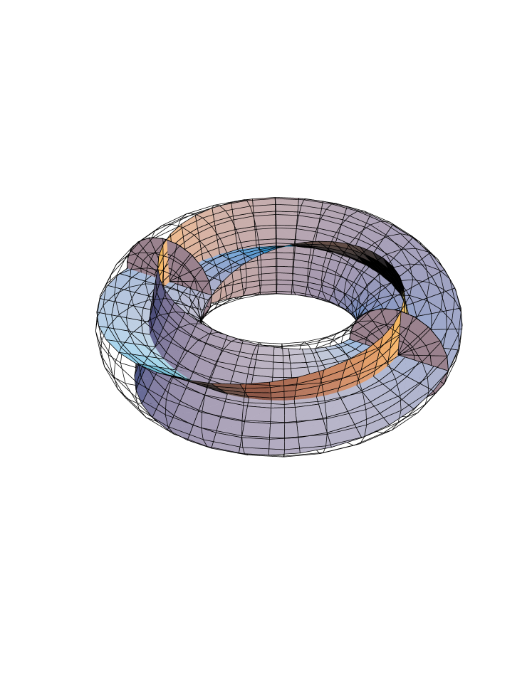
The problem can be reformulated in robotics terms as follows. Consider a mobile robot in the plane that can move forward and backward, and rotate around itself (Reeds-Shepp car). The state of the robot is described by coordinates $(x,y)$ of its center of mass and by angle of orientation $\theta$. Given an initial and a terminal state of the car, one should find the shortest path from the initial state to the terminal one, when the length of the path is measured in the space $(x,y,\theta)$, see Fig. 1.

Figure 1: Problem statement

Cauchy-Schwarz inequality implies that the minimization problem for the sub-Riemannian length functional $(\ref{l})$ is equivalent to the minimization problem for the energy functional

$$J=\frac{1}{2}\int_{0}^{t_{1}}(u_{1}^{2}+u_{2}^{2})\,dt\to\min$$ (2.7)

with fixed $t_{1}$.

System $(\ref{sys2})$ has full rank:

$$\xi_{3}=[\xi_{1},\xi_{2}]=\sin\theta\frac{\partial\,}{\partial\,x}-\cos\theta\frac{\partial\,}{\partial\,y},$$ (2.8)

$$\operatorname{span}\nolimits(\xi_{1}(q),\xi_{2}(q),\xi_{3}(q))=T_{q}M\qquad\forall\ q\in M,$$ (2.9)

so it is completely controllable on $M$.

Another standard reasoning proves existence of solutions to optimal control problem $(\ref{sys2})$, $(\ref{bound})$, $(\ref{J})$. First the problem is equivalently reduced to the time-optimal problem with dynamics $(\ref{sys2})$, boundary conditions $(\ref{bound})$, restrictions on control $u_{1}^{2}+u_{2}^{2}\leq 1$, and the cost functional $t_{1}\to\min$. Then the state space of the problem is embedded into ${\mathbb{R}}^{3}$ (see e.g. [17]), and finally Filippov’s theorem [3] implies existence of optimal controls.

3 Pontryagin Maximum Principle

We apply the version of PMP adapted to left-invariant optimal control problems and use the basic notions of the Hamiltonian formalism as described in [3]. In particular, we denote by $T^{*}M$ the cotangent bundle of a manifold $M$, by $\pi\,:\,T^{*}M\to M$ the canonical projection, and by $\vec{h}\in\operatorname{Vec}\nolimits(T^{*}M)$ the Hamiltonian vector field corresponding to a Hamiltonian function $h\in C^{\infty}(T^{*}M)$.

Consider linear on fibers Hamiltonians corresponding to the vector fields $\xi_{i}$:

$$h_{i}(\lambda)=\langle\lambda,\xi_{i}(q)\rangle,\quad q=\pi(\lambda),\quad\lambda\in T^{*}M,\quad i=1,2,3,$$

and the control-dependent Hamiltonian of PMP

$$h_{u}^{\nu}(\lambda)=\frac{\nu}{2}(u_{1}^{2}+u_{2}^{2})+u_{1}h_{1}(\lambda)+u_{2}h_{2}(\lambda),\quad\lambda\in T^{*}M,\quad u\in{\mathbb{R}}^{2},\quad\nu\in\{-1,0\}.$$

Then the Pontryagin Maximum Principle [12, 3] for the problem under consideration reads as follows.

Theorem 3.1.

Let $u(t)$ and $q(t)$, $t\in[0,t_{1}]$, be an optimal control and the corresponding optimal trajectory in problem $(\ref{sys2})$, $(\ref{bound})$, $(\ref{J})$. Then there exist a Lipschitzian curve $\lambda_{t}\in T^{*}M$, $\pi(\lambda_{t})=q(t)$, $t\in[0,t_{1}]$, and a number $\nu\in\{-1,0\}$ for which the following conditions hold for almost all $t\in[0,t_{1}]$:

$$\dot{\lambda}_{t}=\vec{h}^{\nu}_{u(t)}(\lambda_{t})=u_{1}(t)\vec{h}_{1}(\lambda_{t})+u_{2}(t)\vec{h}_{2}(\lambda_{t}),$$ (3.1)

$$h^{\nu}_{u(t)}(\lambda_{t})=\max_{u\in{\mathbb{R}}^{2}}h^{\nu}_{u}(\lambda_{t}),$$ (3.2)

$$(\nu,\lambda_{t})\neq 0.$$ (3.3)

Relations $(\ref{xi3})$, $(\ref{spanxi123})$ mean that the sub-Riemannian problem under consideration is contact, thus in the abnormal case $\nu=0$ the optimal trajectories are constant.

Consider now the normal case $\nu=-1$. Then the maximality condition $(\ref{PMP2})$ implies that normal extremals satisfy the equalities

$$u_{i}(t)=h_{i}(\lambda_{t}),\qquad i=1,2,$$

thus they are trajectories of the normal Hamiltonian system

$$\dot{\lambda}=\vec{H}(\lambda),\qquad\lambda\in T^{*}M,$$ (3.4)

with the maximized Hamiltonian $H=(h_{1}^{2}+h_{2}^{2})/2$.

In view of the multiplication table

$$[\xi_{1},\xi_{2}]=\xi_{3},\quad[\xi_{1},\xi_{3}]=0,\quad[\xi_{2},\xi_{3}]=\xi_{1},$$

system $(\ref{dlamvH})$ reads in coordinates as follows:

$$\dot{h}_{1}=-h_{2}h_{3},\quad\dot{h}_{2}=h_{1}h_{3},\quad\dot{h}_{3}=h_{2}h_{3},$$ (3.5)

$$\dot{x}=h_{1}\cos\theta,\quad\dot{y}=h_{1}\sin\theta,\quad\dot{\theta}=h_{2}.$$ (3.6)

Along all normal extremals we have $H\equiv C\geq 0$; moreover, for non-constant normal extremal trajectories $C>0$. Since the normal Hamiltonian system $(\ref{dh123})$, $(\ref{dxyth})$ is homogeneous w.r.t. $(h_{1},h_{2})$, we can consider its trajectories only on the level surface $H=1/2$ (this corresponds to the arc-length parametrization of extremal trajectories), and set the terminal time $t_{1}$ free. Then the initial covector $\lambda$ for normal extremals $\lambda_{t}=e^{t\vec{H}}(\lambda)$ belongs to the initial cylinder

$$C=T_{q_{0}}^{*}M\cap\{H(\lambda)=1/2\}.$$

Introduce the polar coordinates

$$h_{1}=\cos\alpha,\quad h_{2}=\sin\alpha,$$

then the initial cylinder decomposes as $C\cong S^{1}_{\alpha}\times{\mathbb{R}}_{h_{3}}$, where $S^{1}_{\alpha}={\mathbb{R}}/(2\pi{\mathbb{Z}})$. In these coordinates the vertical part $(\ref{dh123})$ reads as

$$\dot{\alpha}=h_{3},\quad\dot{h}_{3}=\frac{1}{2}\sin 2\alpha,\quad(\alpha,h_{3})\in C.$$ (3.7)

In the coordinates

$$\gamma=2\alpha+\pi\in 2S^{1}={\mathbb{R}}/(4\pi{\mathbb{Z}}),\qquad c=2h_{3}\in{\mathbb{R}},$$

system $(\ref{dah3})$ takes the form of the standard pendulum

$$\dot{\gamma}=c,\quad\dot{c}=-\sin\gamma,\qquad(\gamma,c)\in C\cong(2S^{1}_{\gamma})\times{\mathbb{R}}_{c}.$$ (3.8)

Here $2S^{1}={\mathbb{R}}/(4\pi{\mathbb{Z}})$ is the double covering of the standard circle $S^{1}={\mathbb{R}}/(2\pi{\mathbb{Z}})$. Then the horizontal part $(\ref{dxyth})$ of the normal Hamiltonian system reads as

$$\dot{x}=\sin\frac{\gamma}{2}\cos\theta,\quad\dot{y}=\sin\frac{\gamma}{2}\sin\theta,\quad\dot{\theta}=-\cos\frac{\gamma}{2}.$$ (3.9)

Summing up, all nonconstant arc-length parametrized optimal trajectories in the sub-Riemannian problem on the Lie group $\operatorname{SE}\nolimits(2)$ are projections of solutions to the normal Hamiltonian system $(\ref{ham_vert})$, $(\ref{ham_hor})$.

4 Exponential mapping

The family of arc-length parametrized normal extremal trajectories is described by the exponential mapping

$$\operatorname{Exp}\nolimits\,:\,N\to M,\qquad N=C\times{\mathbb{R}}_{+},$$

$$\operatorname{Exp}\nolimits(\nu)=\operatorname{Exp}\nolimits(\lambda,t)=\pi\circ e^{t\vec{H}}(\lambda)=\pi(\lambda_{t})=q(t),$$

$$\nu=(\lambda,t)=(\gamma,c,t)\in N.$$

In this section we derive explicit formulas for the exponential mapping in special elliptic coordinates in $C$ induced by the flow of the pendulum $(\ref{ham_vert})$. The general construction of elliptic coordinates was developed in [13, 14, 17], here they are adapted to the problem under consideration.

4.1 Decomposition of the cylinder $C$

The equation of pendulum $(\ref{ham_vert})$ has the energy integral

$$E=\frac{c^{2}}{2}-\cos\gamma\in[-1,+\infty).$$ (4.1)

Consider the following decomposition of the cylinder $C$ into disjoint invariant sets of the pendulum:

$$C=\bigcup_{i=1}^{5}C_{i},$$ (4.2)

$$C_{1}=\{\lambda\in C\mid E\in(-1,1)\},$$

$$C_{2}=\{\lambda\in C\mid E\in(1,+\infty)\},$$

$$C_{3}=\{\lambda\in C\mid E=1,\ c\neq 0\},$$

$$C_{4}=\{\lambda\in C\mid E=-1\}=\{(\gamma,c)\in C\mid\gamma=2\pi n,\ c=0\},$$

$$C_{5}=\{\lambda\in C\mid E=1,\ c=0\}=\{(\gamma,c)\in C\mid\gamma=\pi+2\pi n,\ c=0\}.$$

Here and below we denote by $n$ a natural number.

Denote the connected components of the sets $C_{i}$:

$$C_{1}=\cup_{i=0}^{1}C_{1}^{i},\qquad C_{1}^{i}=\{(\gamma,c)\in C_{1}\mid\operatorname{sgn}\nolimits(\cos(\gamma/2))=(-1)^{i}\},\quad i=0,1,$$

$$C_{2}=C_{2}^{+}\cup C_{2}^{-},\qquad C_{2}^{\pm}=\{(\gamma,c)\in C_{2}\mid\operatorname{sgn}\nolimits c=\pm 1\},$$

$$C_{3}=\cup_{i=0}^{1}(C_{3}^{i+}\cup C_{3}^{i-}),$$

$$\qquad\qquad C_{3}^{i\pm}=\{(\gamma,c)\in C_{3}\mid\operatorname{sgn}\nolimits(\cos(\gamma/2))=(-1)^{i},\ \operatorname{sgn}\nolimits c=\pm 1\},\quad i=0,1,$$

$$C_{4}=\cup_{i=0}^{1}C_{4}^{i},\qquad C_{4}^{i}=\{(\gamma,c)\in C\mid\gamma=2\pi i,\ c=0\},\quad i=0,1,$$

$$C_{5}=\cup_{i=0}^{1}C_{5}^{i},\qquad C_{5}^{i}=\{(\gamma,c)\in C\mid\gamma=\pi+2\pi i,\ c=0\},\quad i=0,1.$$

Decomposition $(\ref{decompC})$ of the cylinder $C$ is shown at Fig. 2.

Figure 2: Decomposition of the cylinder $C$

4.2 Elliptic coordinates on the cylinder $C$

According to the general construction developed in [17], we introduce elliptic coordinates $(\varphi,k)$ on the domain $C_{1}\cup C_{2}\cup C_{3}$ of the cylinder $C$, where $k$ is a reparametrized energy, and $\varphi$ is the time of motion of the pendulum $(\ref{ham_vert})$. We use Jacobi’s functions $\operatorname{am}\nolimits(\varphi,k)$, $\operatorname{cn}\nolimits(\varphi,k)$, $\operatorname{sn}\nolimits(\varphi,k)$, $\operatorname{dn}\nolimits(\varphi,k)$, $\operatorname{E}\nolimits(\varphi,k)$; moreover, $K(k)$ is the complete elliptic integral of the first kind [21].

If $\lambda=(\gamma,c)\in C_{1}$, then:

$$k=\sqrt{\frac{E+1}{2}}=\sqrt{\sin^{2}\frac{\gamma}{2}+\frac{c^{2}}{4}}\in(0,1),$$

$$\sin\frac{\gamma}{2}=s_{1}k\operatorname{sn}\nolimits(\varphi,k),\qquad s_{1}=\operatorname{sgn}\nolimits\cos(\gamma/2),$$

$$\cos\frac{\gamma}{2}=s_{1}\operatorname{dn}\nolimits(\varphi,k),$$

$$\frac{c}{2}=k\operatorname{cn}\nolimits(\varphi,k),\qquad\varphi\in[0,4K(k)].$$

If $\lambda=(\gamma,c)\in C_{2}$, then:

$$k=\sqrt{\frac{2}{E+1}}=\frac{1}{\sqrt{\sin^{2}\frac{\gamma}{2}+\frac{c^{2}}{4}}}\in(0,1),$$

$$\sin\frac{\gamma}{2}=s_{2}\operatorname{sn}\nolimits(\varphi/k,k),\qquad s_{2}=\operatorname{sgn}\nolimits c,$$

$$\cos\frac{\gamma}{2}=\operatorname{cn}\nolimits(\varphi/k,k),$$

$$\frac{c}{2}=(s_{2}/k)\operatorname{dn}\nolimits(\varphi/k,k),\qquad\varphi\in[0,4kK(k)].$$

If $\lambda=(\gamma,c)\in C_{3}$, then:

$$k=1,$$

$$\sin\frac{\gamma}{2}=s_{1}s_{2}\tanh\varphi,\qquad s_{1}=\operatorname{sgn}\nolimits\cos(\gamma/2),\quad s_{2}=\operatorname{sgn}\nolimits c,$$

$$\cos\frac{\gamma}{2}=s_{1}/\cosh\varphi,$$

$$\frac{c}{2}=s_{2}/\cosh\varphi,\qquad\varphi\in(-\infty,+\infty).$$

4.3 Parametrization of extremal trajectories

In the elliptic coordinates the flow of the pendulum $(\ref{ham_vert})$ rectifies:

$$\dot{\varphi}=1,\quad\dot{k}=0,\qquad\lambda=(\varphi,k)\in\cup_{i=1}^{3}C_{i},$$

this is verified directly using the formulas of Subsec. 4.2. Thus the vertical subsystem of the normal Hamiltonian system of PMP $(\ref{ham_vert})$ is trivially integrated: one should just substitute $\varphi_{t}=\varphi+t$, $k\equiv\operatorname{const}\nolimits$ to the formulas of elliptic coordinates of Subsec. 4.2. Integrating the horizontal subsystem $(\ref{ham_hor})$, we obtain the following parametrization of extremal trajectories.

If $\lambda=(\varphi,k)\in C_{1}$, then $\varphi_{t}=\varphi+t$ and:

$$\cos\theta_{t}=\operatorname{cn}\nolimits\varphi\operatorname{cn}\nolimits\varphi_{t}+\operatorname{sn}\nolimits\varphi\operatorname{sn}\nolimits\varphi_{t},$$

$$\sin\theta_{t}=s_{1}(\operatorname{sn}\nolimits\varphi\operatorname{cn}\nolimits\varphi_{t}-\operatorname{cn}\nolimits\varphi\operatorname{sn}\nolimits\varphi_{t}),$$

$$\theta_{t}=s_{1}(\operatorname{am}\nolimits\varphi-\operatorname{am}\nolimits\varphi_{t})\pmod{2\pi},$$

$$x_{t}=(s_{1}/k)[\operatorname{cn}\nolimits\varphi(\operatorname{dn}\nolimits\varphi-\operatorname{dn}\nolimits\varphi_{t})+\operatorname{sn}\nolimits\varphi(t+\operatorname{E}\nolimits(\varphi)-\operatorname{E}\nolimits(\varphi_{t}))],$$

$$y_{t}=(1/k)[\operatorname{sn}\nolimits\varphi(\operatorname{dn}\nolimits\varphi-\operatorname{dn}\nolimits\varphi_{t})-\operatorname{cn}\nolimits\varphi(t+\operatorname{E}\nolimits(\varphi)-\operatorname{E}\nolimits(\varphi_{t}))].$$

In the domain $C_{2}$, it will be convenient to use the coordinate

$$\psi=\varphi/k,\qquad\psi_{t}=\varphi_{t}/k=\psi+t/k.$$

If $\lambda\in C_{2}$, then:

$$\cos\theta_{t}=k^{2}\operatorname{sn}\nolimits\psi\operatorname{sn}\nolimits\psi_{t}+\operatorname{dn}\nolimits\psi\operatorname{dn}\nolimits\psi_{t},$$

$$\sin\theta_{t}=k(\operatorname{sn}\nolimits\psi\operatorname{dn}\nolimits\psi_{t}-\operatorname{dn}\nolimits\psi\operatorname{sn}\nolimits\psi_{t}),$$

$$x_{t}=s_{2}k[\operatorname{dn}\nolimits\psi(\operatorname{cn}\nolimits\psi-\operatorname{cn}\nolimits\psi_{t})+\operatorname{sn}\nolimits\psi(t/k+\operatorname{E}\nolimits(\psi)-\operatorname{E}\nolimits(\psi_{t}))],$$

$$y_{t}=s_{2}[k^{2}\operatorname{sn}\nolimits\psi(\operatorname{cn}\nolimits\psi-\operatorname{cn}\nolimits\psi_{t})-\operatorname{dn}\nolimits\psi(t/k+\operatorname{E}\nolimits(\psi)-\operatorname{E}\nolimits(\psi_{t}))].$$

If $\lambda\in C_{3}$, then:

$$\cos\theta_{t}=1/(\cosh\varphi\cosh\varphi_{t})+\tanh\varphi\tanh\varphi_{t},$$

$$\sin\theta_{t}=s_{1}(\tanh\varphi/\cosh\varphi_{t}-\tanh\varphi_{t}/\cosh\varphi),$$

$$x_{t}=s_{1}s_{2}[(1/\cosh\varphi)(1/\cosh\varphi-1/\cosh\varphi_{t})+\tanh\varphi(t+\tanh\varphi-\tanh\varphi_{t})],$$

$$y_{t}=s_{2}[\tanh\varphi(1/\cosh\varphi-1/\cosh\varphi_{t})-(1/\cosh\varphi)(t+\tanh\varphi-\tanh\varphi_{t})].$$

In the degenerate cases, the normal Hamiltonian system $(\ref{ham_vert})$, $(\ref{ham_hor})$ is easily integrated.

If $\lambda\in C_{4}$, then:

$$\theta_{t}=-s_{1}t,\qquad x_{t}=0,\qquad y_{t}=0.$$

If $\lambda\in C_{5}$, then:

$$\theta_{t}=0,\qquad x_{t}=t\,\operatorname{sgn}\nolimits\sin(\gamma/2),\qquad y_{t}=0.$$

It is easy to compute from the Hamiltonian system $(\ref{ham_vert})$, $(\ref{ham_hor})$ that projections $(x_{t},y_{t})$ of extremal trajectories have curvature $\kappa=-\cot(\gamma_{t}/2)$. Thus they have inflection points when $\cos(\gamma_{t}/2)=0$, and cusps when $\sin(\gamma_{t}/2)=0$. Each curve $(x_{t},y_{t})$ for $\lambda\in\cup_{i=1}^{3}C_{i}$ has cusps. In the case $\lambda\in C_{1}\cup C_{3}$ these curves have no inflection points, and in the case $\lambda\in C_{2}$ each such curve has inflection points. Plots of the curves $(x_{t},y_{t})$ in the cases $\lambda\in C_{1}\cup C_{2}\cup C_{3}$ are given respectively at Figs. 4, 4, 5.

Figure 3: Non-inflexional trajectory: $\lambda\in C_{1}$

Figure 4: Inflexional trajectory: $\lambda\in C_{2}$

Figure 5: Critical trajectory: $\lambda\in C_{3}$

In the cases $\lambda\in C_{4}$ and $\lambda\in C_{5}$ the extremal trajectories $q_{t}$ are respectively Riemannian geodesics in the circle $\{x=y=0\}$ and in the plane $\{\theta=0\}$.

5 Discrete symmetries and Maxwell strata

In this section we continue reflections in the state cylinder of the standard pendulum to discrete symmetries of the exponential mapping.

5.1 Symmetries of the vertical part of Hamiltonian system

5.1.1 Reflections in the state cylinder of pendulum

The phase portrait of pendulum $(\ref{ham_vert})$ admits the following reflections:

$$\varepsilon^{1}\,:\,(\gamma,c)\to(\gamma,-c),$$

$$\varepsilon^{2}\,:\,(\gamma,c)\to(-\gamma,c),$$

$$\varepsilon^{3}\,:\,(\gamma,c)\to(-\gamma,-c),$$

$$\varepsilon^{4}\,:\,(\gamma,c)\to(\gamma+2\pi,c),$$

$$\varepsilon^{5}\,:\,(\gamma,c)\to(\gamma+2\pi,-c),$$

$$\varepsilon^{6}\,:\,(\gamma,c)\to(-\gamma+2\pi,c),$$

$$\varepsilon^{7}\,:\,(\gamma,c)\to(-\gamma+2\pi,-c).$$

These reflections generate the group of symmetries of a parallelepiped $G=\{\operatorname{Id}\nolimits,\varepsilon^{1},\dots,\varepsilon^{7}\}$. The reflections $\varepsilon^{3}$, $\varepsilon^{4}$, $\varepsilon^{7}$ preserve direction of time on trajectories of pendulum, while the reflections $\varepsilon^{1}$, $\varepsilon^{2}$, $\varepsilon^{5}$, $\varepsilon^{6}$ reverse the direction of time.

5.1.2 Reflections of trajectories of pendulum

Proposition 5.1.

The following mappings transform trajectories of pendulum $(\ref{ham_vert})$ to trajectories:

$$\varepsilon^{i}\,:\,\delta=\{(\gamma_{s},c_{s})\mid s\in[0,t]\}\mapsto\delta^{i}=\{(\gamma_{s}^{i},c_{s}^{i})\mid s\in[0,t]\},\quad i=1,\dots,7,$$ (5.1)

where

$$(\gamma_{s}^{1},c_{s}^{1})=(\gamma_{t-s},-c_{t-s}),$$

$$(\gamma_{s}^{2},c_{s}^{2})=(-\gamma_{t-s},c_{t-s}),$$

$$(\gamma_{s}^{3},c_{s}^{3})=(-\gamma_{s},-c_{s}),$$

$$(\gamma_{s}^{4},c_{s}^{4})=(\gamma_{s}+2\pi,c_{s}),$$

$$(\gamma_{s}^{5},c_{s}^{5})=(\gamma_{t-s}+2\pi,-c_{t-s}),$$

$$(\gamma_{s}^{6},c_{s}^{6})=(-\gamma_{t-s}+2\pi,c_{t-s}),$$

$$(\gamma_{s}^{7},c_{s}^{7})=(-\gamma_{s}+2\pi,-c_{s}).$$

Proof.

The statement is verified by substitution to system $(\ref{ham_vert})$ and differentiation. ∎

The action $(\ref{epsi_delta})$ of reflections $\varepsilon^{i}$ on trajectories $\delta$ of the pendulum $(\ref{ham_vert})$ is illustrated at Fig. 6.

Figure 6: Reflections $\varepsilon^{i}\,:\,\delta\mapsto\delta^{i}$ of trajectories of pendulum

5.2 Symmetries of Hamiltonian system

5.2.1 Reflections of extremals

We define action of the group $G$ on the normal extremals $\lambda_{s}=e^{s\vec{H}}(\lambda_{0})\in T^{*}M$, $s\in[0,t]$, i.e., solutions to the normal Hamiltonian system

$$\dot{\gamma}_{s}=c_{s},\qquad\dot{c}_{s}=-\sin\gamma_{s},$$ (5.2)

$$\dot{q}_{s}=\sin\frac{\gamma_{s}}{2}\,X_{1}(q_{s})-\cos\frac{\gamma_{s}}{2}\,X_{2}(q_{s})$$ (5.3)

as follows:

$$\varepsilon^{i}\,:\,\{\lambda_{s}\mid s\in[0,t]\}\mapsto\{\lambda_{s}^{i}\mid s\in[0,t]\},\qquad i=1,\dots,7,$$ (5.4)

$$\lambda_{s}=(\gamma_{s},c_{s},q_{s}),\qquad\lambda_{s}^{i}=(\gamma_{s}^{i},c_{s}^{i},q_{s}^{i}).$$ (5.5)

Here $\lambda_{s}^{i}$ is a solution to the Hamiltonian system $(\ref{Ham_s1})$, $(\ref{Ham_s2})$, and the action of reflections on the vertical coordinates $(\gamma_{s},c_{s})$ was defined in Subsec. 5.1. The action of reflections on the horizontal coordinates $(x_{s},y_{s},\theta_{s})$ is described as follows.

Proposition 5.2.

Let $q_{s}=(x_{s},y_{s},\theta_{s})$, $s\in[0,t]$, be a normal extremal trajectory, and let $q_{s}^{i}=(x_{s}^{i},y_{s}^{i},\theta_{s}^{i})$, $s\in[0,t]$, be its image under the action of the reflection $\varepsilon^{i}$ as defined by $(\ref{epsilam})$, $(\ref{lamsgams})$. Then the following equalities hold:

$$(1) \theta_{1}^{s}=\theta_{t}-\theta_{t-s},$$

$$x^{1}_{s}=\cos\theta_{t}(x_{t}-x_{t-s})+\sin\theta_{t}(y_{t}-y_{t-s}),$$

$$y^{1}_{s}=\sin\theta_{t}(x_{t}-x_{t-s})-\cos\theta_{t}(y_{t}-y_{t-s}),$$

$$(2) \theta_{2}^{s}=\theta_{t}-\theta_{t-s},$$

$$x^{2}_{s}=-\cos\theta_{t}(x_{t}-x_{t-s})-\sin\theta_{t}(y_{t}-y_{t-s}),$$

$$y^{2}_{s}=-\sin\theta_{t}(x_{t}-x_{t-s})+\cos\theta_{t}(y_{t}-y_{t-s}),$$

$$(3) \theta_{3}^{s}=\theta_{s},$$

$$x^{3}_{s}=-x_{s},$$

$$y^{3}_{s}=-y_{s},$$

$$(4) \theta_{4}^{s}=-\theta_{s},$$

$$x^{4}_{s}=-x_{s},$$

$$y^{4}_{s}=y_{s},$$

$$(5) \theta_{5}^{s}=\theta_{t-s}-\theta_{t},$$

$$x^{5}_{s}=\cos\theta_{t}(x_{t-s}-x_{t})+\sin\theta_{t}(y_{t-s}-y_{t}),$$

$$y^{5}_{s}=-\sin\theta_{t}(x_{t-s}-x_{t})+\cos\theta_{t}(y_{t-s}-y_{t}),$$

$$(6) \theta_{6}^{s}=\theta_{t-s}-\theta_{t},$$

$$x^{6}_{s}=\cos\theta_{t}(x_{t}-x_{t-s})+\sin\theta_{t}(y_{t}-y_{t-s}),$$

$$y^{6}_{s}=-\sin\theta_{t}(x_{t}-x_{t-s})+\cos\theta_{t}(y_{t}-y_{t-s}),$$

$$(7) \theta_{7}^{s}=-\theta_{s},$$

$$x^{7}_{s}=x_{s},$$

$$y^{7}_{s}=-y_{s}.$$

Proof.

We prove only the formulas for $\theta^{1}_{s}$ and $x^{1}_{s}$ since all other equalities are proved similarly.

By Proposition 5.1, we have $\gamma_{s}^{1}=\gamma_{t-s}$. Then we obtain from $(\ref{ham_vert})$:

$$\theta^{1}_{s}=\int_{0}^{s}-\cos\frac{\gamma^{1}_{r}}{2}\,dr=-\int_{0}^{s}\cos\frac{\gamma_{t-r}}{2}\,dr=\int_{t}^{t-s}\cos\frac{\gamma_{p}}{2}\,dp=\theta_{t}-\theta_{t-s}$$

and

$$x^{1}_{s} =\int_{0}^{s}\sin\frac{\gamma^{1}_{r}}{2}\cos\theta^{1}_{r}\,dr=\int_{0}^{s}\sin\frac{\gamma_{t-r}}{2}\cos(\theta_{t}-\theta_{t-r})\,dr$$

$$=-\cos\theta_{t}\int_{t}^{t-s}\sin\frac{\gamma_{p}}{2}\cos\theta_{p}\,dp-\sin\theta_{t}\int_{t}^{t-s}\sin\frac{\gamma_{p}}{2}\sin\theta_{p}\,dp$$

$$=\cos\theta_{t}(x_{t}-x_{t-s})+\sin\theta_{t}(y_{t}-y_{t-s}).$$

∎

The action of reflections $\varepsilon^{i}$ on curves $(x_{s},y_{s})$ has a simple visual meaning. Up to rotations of the plane $(x,y)$, the mappings $\varepsilon^{1}$, $\varepsilon^{2}$, $\varepsilon^{3}$ are respectively reflections of the curves $\{(x_{s},y_{s})\mid s\in[0,t]\}$ in the center of the segment $l$ connecting the endpoints $(x_{0},y_{0})$ and $(x_{t},y_{t})$, in the middle perpendicular to $l$, and in $l$ itself (see [14, 17]). The mapping $\varepsilon^{4}$ is the reflection in the axis $y$ perpendicular to the initial velocity vector $(\cos\theta_{0},\sin\theta_{0})$. The rest mappings are represented as follows: $\varepsilon^{i+4}=\varepsilon^{4}\circ\varepsilon^{i}$, $i=1,2,3$.

5.2.2 Reflections of endpoints of extremal trajectories

We define action of reflections in the state space $M$ as the action on endpoints of extremal trajectories

$$\varepsilon^{i}\,:\,M\to M,\qquad\varepsilon^{i}\,:\,q_{t}\mapsto q^{i}_{t},$$ (5.6)

see $(\ref{epsilam})$, $(\ref{lamsgams})$. By virtue of Propos. 5.2, the point $q_{t}^{i}$ depends only on the endpoint $q_{t}$, not on the whole trajectory $\{q_{s}\mid s\in[0,t]\}$.

Proposition 5.3.

Let $q=(x,y,\theta)\in M$, $q^{i}=\varepsilon^{i}(q)=(x^{i},y^{i},\theta^{i})\in M$. Then:

$$(x^{1},y^{1},\theta^{1})=(x\cos\theta+y\sin\theta,x\sin\theta-y\cos\theta,\theta),$$

$$(x^{2},y^{2},\theta^{2})=(-x\cos\theta-y\sin\theta,-x\sin\theta+y\cos\theta,\theta),$$

$$(x^{3},y^{3},\theta^{3})=(-x,-y,\theta),$$

$$(x^{4},y^{4},\theta^{4})=(-x,y,-\theta),$$

$$(x^{5},y^{5},\theta^{5})=(-x\cos\theta-y\sin\theta,x\sin\theta-y\cos\theta,-\theta),$$

$$(x^{6},y^{6},\theta^{6})=(x\cos\theta+y\sin\theta,-x\sin\theta+y\cos\theta,-\theta),$$

$$(x^{7},y^{7},\theta^{7})=(x,-y,-\theta).$$

Proof.

It suffices to substitute $s=0$ to the formulas of Proposition 5.2. ∎

5.3 Reflections as symmetries of exponential mapping

Define action of the reflections in the preimage of the exponential mapping:

$$\varepsilon^{i}\,:\,N\to N,\qquad\varepsilon^{i}\,:\,\nu=(\gamma,c,t)\mapsto\nu^{i}=(\gamma^{i},c^{i},t),$$ (5.7)

where $(\gamma,c)=(\gamma_{0},c_{0})$ and $(\gamma^{i},c^{i})=(\gamma^{i}_{0},c^{i}_{0})$ are the initial points of the corresponding trajectories of pendulum $(\gamma_{s},c_{s})$ and $(\gamma_{s}^{i},c_{s}^{i})$. The explicit formulas for $(\gamma^{i},c^{i})$ are given by the following statement.

Proposition 5.4.

Let $\nu=(\lambda,t)=(\gamma,c,t)\in N$, $\nu^{i}=\varepsilon^{i}(\nu)=(\lambda^{i},t)=(\gamma^{i},c^{i},t)\in N$. Then:

$$(\gamma^{1},c^{1})=(\gamma_{t},-c_{t}),$$

$$(\gamma^{2},c^{2})=(-\gamma_{t},c_{t}),$$

$$(\gamma^{3},c^{3})=(-\gamma,-c),$$

$$(\gamma^{4},c^{4})=(\gamma+2\pi,c),$$

$$(\gamma^{5},c^{5})=(\gamma_{t}+2\pi,-c_{t}),$$

$$(\gamma^{6},c^{6})=(-\gamma_{t}+2\pi,c_{t}),$$

$$(\gamma^{7},c^{7})=(-\gamma,-c).$$

Proof.

Apply Proposition 5.1 with $s=0$. ∎

Formulas $(\ref{epsiq})$, $(\ref{epsinu})$ define the action of reflections $\varepsilon^{i}$ in the image and preimage of the exponential mapping. Since the both actions of $\varepsilon^{i}$ in $M$ and $N$ are induced by the action of $\varepsilon^{i}$ on extremals $\lambda_{s}$ $(\ref{epsilam})$, we obtain the following statement.

Proposition 5.5.

For any $i=1,\dots,7$, the reflection $\varepsilon^{i}$ is a symmetry of the exponential mapping, i.e., the following diagram is commutative:

                  

6 Maxwell strata corresponding to reflections

6.1 Maxwell points and optimality
of extremal trajectories

A point $q_{t}$ of a sub-Riemannian geodesic is called a Maxwell point if there exists another extremal trajectory $\widetilde{q}_{s}\not\equiv q_{s}$ such that $\widetilde{q}_{t}=q_{t}$ for the instant of time $t>0$. It is well known that after a Maxwell point a sub-Riemannian geodesic cannot be optimal (provided the problem is analytic).

In this section we compute Maxwell points corresponding to reflections. For any $i=1,\dots,7$, define the Maxwell stratum in the preimage of the exponential mapping corresponding to the reflection $\varepsilon^{i}$ as follows:

$$\operatorname{MAX}\nolimits^{i}=\{\nu=(\lambda,t)\in N\mid\lambda\neq\lambda^{i},\ \operatorname{Exp}\nolimits(\lambda,t)=\operatorname{Exp}\nolimits(\lambda^{i},t)\}.$$ (6.1)

We denote the corresponding Maxwell stratum in the image of the exponential mapping as

$$\operatorname{Max}\nolimits^{i}=\operatorname{Exp}\nolimits(\operatorname{MAX}\nolimits^{i})\subset M.$$

If $\nu=(\lambda,t)\in\operatorname{MAX}\nolimits^{i}$, then $q_{t}=\operatorname{Exp}\nolimits(\nu)\in\operatorname{Max}\nolimits^{i}$ is a Maxwell point along the trajectory $q_{s}=\operatorname{Exp}\nolimits(\lambda,s)$. Here we use the fact that if $\lambda\neq\lambda^{i}$, then $\operatorname{Exp}\nolimits(\lambda,s)\not\equiv\operatorname{Exp}\nolimits(\lambda^{i},s)$.

6.2 Multiple points of exponential mapping

In this subsection we study solutions to the equation $q=q^{i}$, where $q^{i}=\varepsilon^{i}(q)$, that appears in definition $(\ref{MAX_def})$ of Maxwell strata $\operatorname{MAX}\nolimits^{i}$.

The following functions are defined on $M={\mathbb{R}}^{2}_{x,y}\times S^{1}_{\theta}$ up to sign:

$$R_{1}=y\cos\frac{\theta}{2}-x\sin\frac{\theta}{2},\qquad R_{2}=x\cos\frac{\theta}{2}+x\sin\frac{\theta}{2},$$

although their zero sets $\{R_{i}=0\}$ are well-defined. In the polar coordinates

$$x=\rho\cos\chi,\qquad y=\rho\sin\chi,$$

these functions read as

$$R_{1}=\rho\sin\left(\chi-\frac{\theta}{2}\right),\qquad R_{2}=\rho\cos\left(\chi-\frac{\theta}{2}\right).$$

Proposition 6.1.

• $q^{1}=q\quad\Leftrightarrow\quad R_{1}(q)=0.$

• $q^{2}=q\quad\Leftrightarrow\quad R_{2}(q)=0.$

• $q^{3}=q\quad\Leftrightarrow\quad x=y=0.$

• $q^{4}=q\quad\Leftrightarrow\quad\sin\theta=x=0.$

• $q^{5}=q\quad\Leftrightarrow\quad\theta=\pi\text{ or }(x,y,\theta)=(0,0,0).$

• $q^{6}=q\quad\Leftrightarrow\quad\theta=0.$

• $q^{7}=q\quad\Leftrightarrow\quad\sin\theta=y=0.$

Proof.

We prove only item (1), all the rest items are considered similarly. By virtue of Proposition 5.3, we have

$$q^{1}=q \quad\Leftrightarrow\quad\begin{cases}x\cos\theta+y\sin\theta=x\\ x\sin\theta-y\cos\theta=y\end{cases}\quad\Leftrightarrow\quad\begin{cases}\rho\sin\frac{\theta}{2}\sin\left(\chi-\frac{\theta}{2}\right)=0\\ \rho\cos\frac{\theta}{2}\sin\left(\chi-\frac{\theta}{2}\right)=0\end{cases}$$

$$\quad\Leftrightarrow\quad\rho\sin\left(\chi-\frac{\theta}{2}\right)\quad\Leftrightarrow\quad R_{1}(q)=0.$$

∎

Proposition 6.1 implies that all Maxwell strata corresponding to reflections satisfy the inclusion

$$\operatorname{Max}\nolimits^{i}\subset\{q\in M\mid R_{1}(q)R_{2}(q)\sin\theta=0\}.$$

The equations $R_{i}(q)=0$, $i=1,2$, define two Moebius strips, while the equation $\sin\theta=0$ determines two discs in the state space $M={\mathbb{R}}^{2}_{x,y}\times S^{1}_{\theta}$, see Fig. 7.

Figure 7: Surfaces containing Maxwell strata $\operatorname{Max}\nolimits^{i}$

By virtue of Propos. 6.1, the Maxwell strata $\operatorname{Max}\nolimits^{3}$, $\operatorname{Max}\nolimits^{4}$, $\operatorname{Max}\nolimits^{7}$ are one-dimensional and are contained in the two-dimensional strata $\operatorname{Max}\nolimits^{1}$, $\operatorname{Max}\nolimits^{2}$, $\operatorname{Max}\nolimits^{5}$, $\operatorname{Max}\nolimits^{6}$. Thus in the sequel we restrict ourselves only by the 2-dimensional strata.

6.3 Fixed points of reflections
in preimage of exponential mapping

In this subsection we describe solutions to the equations $\lambda=\lambda^{1}$ essential for explicit characterization of the Maxwell strata $\operatorname{MAX}\nolimits^{i}$, see $(\ref{MAX_def})$.

From now on we will widely use the following variables in the sets $N_{i}$, $i=1,2,3$:

$$\nu=(\lambda,t)\in N_{1}\quad\Rightarrow\quad \tau=(\varphi+\varphi_{t})/2, p=t/2,$$

$$\nu=(\lambda,t)\in N_{2}\quad\Rightarrow\quad \tau=(\varphi+\varphi_{t})/(2k), p=t/(2k),$$

$$\nu=(\lambda,t)\in N_{3}\quad\Rightarrow\quad \tau=(\varphi+\varphi_{t})/2, p=t/2.$$

Proposition 6.2.

Let $(\lambda,t)\in N$, $\varepsilon^{i}(\lambda,t)=(\lambda^{i},t)\in N$. Then:

• $\lambda^{1}=\lambda\quad\Leftrightarrow\quad\begin{cases}\,{\operatorname{cn}\nolimits\tau}\,=0,&\lambda\in C_{1},\\ \text{is impossible for}&\lambda\in C_{2}\cup C_{3},\end{cases}$

• $\lambda^{2}=\lambda\quad\Leftrightarrow\quad\begin{cases}\,{\operatorname{sn}\nolimits\tau}\,=0,&\lambda\in C_{1}\cup C_{2},\\ \tau=0&\lambda\in C_{3},\end{cases}$

• $\lambda^{5}=\lambda$ is impossible,

• $\lambda^{6}=\lambda\quad\Leftrightarrow\quad\begin{cases}\text{is impossible for}&\lambda\in C_{1}\cup C_{3},\\ \,{\operatorname{cn}\nolimits\tau}\,=0,&\lambda\in C_{2}.\end{cases}$

Proof.

We prove only item (1), all other items are proved similarly.

By Propos. 5.4, if $\lambda\in C^{i}_{1}$, then $\lambda^{1}\in C^{i}_{1}$, $i=0,1$. Moreover,

$$\lambda^{1}=\lambda\quad\Leftrightarrow\quad\begin{cases}\gamma_{t}=\gamma\\ -c_{t}=c\end{cases}\quad\Leftrightarrow\quad\begin{cases}\operatorname{sn}\nolimits\varphi_{t}=\operatorname{sn}\nolimits\varphi\\ -\operatorname{cn}\nolimits\varphi_{t}=\operatorname{cn}\nolimits\varphi\end{cases}\quad\Leftrightarrow\quad\,{\operatorname{cn}\nolimits\tau}\,=0.$$

If $\lambda\in C_{2}^{\pm}$, then $\lambda^{1}\in C_{2}^{\mp}$, thus the equality $\lambda^{1}=\lambda$ is impossible.

Similarly, if $\lambda\in C_{3}^{i\pm}$, then $\lambda^{1}\in C_{3}^{i\mp}$, $i=0,1$, and the equality $\lambda^{1}=\lambda$ is impossible. ∎

6.4 General description of Maxwell strata
generated by reflections

We summarize our computations of the previous subsections.

Theorem 6.1.

Let $\nu=(\lambda,t)\in\cup_{i=1}^{3}N_{i}$ and $q_{t}=(x_{t},y_{t},\theta_{t})=\operatorname{Exp}\nolimits(\nu)$.

• $\nu\in\operatorname{MAX}\nolimits^{1}\quad\Leftrightarrow\quad\begin{cases}R_{1}(q_{t})=0,\ \,{\operatorname{cn}\nolimits\tau}\,\neq 0,&\text{for }\lambda\in C_{1},\\ R_{1}(q_{t})=0,&\text{for }\lambda\in C_{2}\cup C_{3}.\end{cases}$

• $\nu\in\operatorname{MAX}\nolimits^{2}\quad\Leftrightarrow\quad R_{2}(q_{t})=0,\ \,{\operatorname{sn}\nolimits\tau}\,\neq 0.$

• $\nu\in\operatorname{MAX}\nolimits^{5}\quad\Leftrightarrow\quad\theta_{t}=\pi\text{ or }(x_{t},y_{t},\theta_{t})=(0,0,0).$

• $\nu\in\operatorname{MAX}\nolimits^{6}\quad\Leftrightarrow\quad\begin{cases}\theta_{t}=0,&\text{for }\lambda\in C_{1}\cup C_{3},\\ \theta_{t}=0,\ \,{\operatorname{cn}\nolimits\tau}\,\neq 0&\text{for }\lambda\in C_{2}.\end{cases}$

Proof.

Apply Propositions 6.1 and 6.2. ∎

6.5 Complete description of Maxwell strata

We obtain bounds for roots of the equations $R_{i}(q_{t})=0$, $\sin\theta_{t}=0$ that appear in the description of Maxwell strata given in Th. 6.1.

We use the following representations of functions along extremal trajectories obtained by direct computation.

If $\lambda\in C_{1}$, then

$$\sin\theta_{t}=-s_{1}\cdot 2\,{\operatorname{cn}\nolimits p}\,\,{\operatorname{sn}\nolimits p}\,\,{\operatorname{dn}\nolimits\tau}\,/\Delta,$$ (6.2)

$$\cos(\theta_{t}/2)=s_{3}\cdot\,{\operatorname{cn}\nolimits p}\,/\sqrt{\Delta},$$ (6.3)

$$\sin(\theta_{t}/2)=s_{4}\cdot\,{\operatorname{sn}\nolimits p}\,\,{\operatorname{dn}\nolimits\tau}\,/\sqrt{\Delta},$$ (6.4)

$$R_{1}(q_{t})=-s_{3}\cdot 2(p-\operatorname{E}\nolimits(p))\,{\operatorname{cn}\nolimits\tau}\,/(k\sqrt{\Delta}),$$ (6.5)

$$R_{2}(q_{t})=-s_{4}\cdot 2f_{2}(p,k)\,{\operatorname{sn}\nolimits\tau}\,/(k\sqrt{\Delta}),$$ (6.6)

$$f_{2}(p,k)=k^{2}\,{\operatorname{cn}\nolimits p}\,\,{\operatorname{sn}\nolimits p}\,-\,{\operatorname{dn}\nolimits p}\,(p-\operatorname{E}\nolimits(p)),$$

$$\Delta=1-k^{2}\,{\operatorname{sn}\nolimits^{2}p}\,\,{\operatorname{dn}\nolimits^{2}\tau}\,,$$

$$s_{3}=\pm 1,\quad s_{4}=\pm 1,\quad s_{1}=-s_{3}s_{4}.$$

If $\lambda\in C_{2}$, then

$$\sin\theta_{t}=-2k\,{\operatorname{sn}\nolimits p}\,\,{\operatorname{dn}\nolimits p}\,\,{\operatorname{cn}\nolimits\tau}\,/\Delta,$$ (6.7)

$$\cos(\theta_{t}/2)=s_{3}\cdot\,{\operatorname{dn}\nolimits p}\,/\sqrt{\Delta},$$ (6.8)

$$\sin(\theta_{t}/2)=s_{4}\cdot k\,{\operatorname{sn}\nolimits p}\,\,{\operatorname{cn}\nolimits\tau}\,/\sqrt{\Delta},$$ (6.9)

$$R_{1}(q_{t})=s_{2}s_{4}\cdot 2(p-\operatorname{E}\nolimits(p))\,{\operatorname{dn}\nolimits\tau}\,/\sqrt{\Delta},$$ (6.10)

$$R_{2}(q_{t})=s_{2}s_{4}\cdot 2kf_{1}(p,k)\,{\operatorname{sn}\nolimits\tau}\,/\sqrt{\Delta},$$ (6.11)

$$f_{1}(p,k)=\,{\operatorname{cn}\nolimits p}\,(\operatorname{E}\nolimits(p)-p)-\,{\operatorname{dn}\nolimits p}\,\,{\operatorname{sn}\nolimits p}\,,$$ (6.12)

$$s_{3}=-s_{4}=\pm 1.$$

Proposition 6.3.

Let $t>0$.

• If $\lambda\in C_{1}$, then $\theta_{t}=0\quad\Leftrightarrow\quad p=2Kn$.

• If $\lambda\in C_{2}$, then $\theta_{t}=0\quad\Leftrightarrow\quad(p=2Kn\text{ or }\,{\operatorname{cn}\nolimits\tau}\,=0)$.

• If $\lambda\in C_{3}$, then $\theta_{t}=0$ is impossible.

Proof.

Apply $(\ref{sinth2C1})$ in item (1), $(\ref{sinth2C2})$ in item (2), and pass to the limit $k\to 1-0$ in item (3). ∎

Proposition 6.4.

Let $t>0$.

• If $\lambda\in C_{1}$, then $\theta_{t}=\pi\quad\Leftrightarrow\quad p=K+2Kn$.

• If $\lambda\in C_{2}$, then $\theta_{t}=\pi$ is impossible.

• If $\lambda\in C_{3}$, then $\theta_{t}=\pi$ is impossible.

Proof.

Apply $(\ref{costh2C1})$ in item (1), $(\ref{costh2C2})$ in item (2), and pass to the limit $k\to 1-0$ in item (3). ∎

Lemma 6.1.

For any $k\in(0,1)$ and any $p>0$ we have $p-\operatorname{E}\nolimits(p)>0$.

Proof.

$\displaystyle p-\operatorname{E}\nolimits(p)=p-\int_{0}^{p}\operatorname{dn}\nolimits^{2}t\,dt=k^{2}\int_{0}^{p}\operatorname{sn}\nolimits^{2}t\,dt>0$. ∎

Proposition 6.5.

Let $t>0$.

• If $\lambda\in C_{1}$, then $R_{1}(q_{t})=0\quad\Leftrightarrow\quad\,{\operatorname{cn}\nolimits\tau}\,=0$.

• If $\lambda\in C_{2}$, then $R_{1}(q_{t})=0$ is impossible.

• If $\lambda\in C_{3}$, then $R_{1}(q_{t})=0$ is impossible.

Proof.

Apply $(\ref{R1C1})$ and Lemma 6.1 in item (1); $(\ref{R1C2})$ and Lemma 6.1 in item (2); and pass to the limit $k\to 1-0$ in item (3). ∎

Lemma 6.2.

For any $k\in(0,1)$ and $p>0$ we have $f_{2}(p,k)>0$.

Proof.

The function $f_{2}(p)$ has the same zeros as the function $g_{2}(p)=f_{2}(p)/\,{\operatorname{dn}\nolimits p}\,$. But $g_{2}(p)>0$ for $p>0$ since $g_{2}(0)=0$ and $g_{2}^{\prime}(p)=k^{2}\,{\operatorname{cn}\nolimits^{2}p}\,/\,{\operatorname{dn}\nolimits^{2}p}\,\geq 0$. ∎

Lemma 6.3.

For any $k\in[0,1)$, the function $f_{1}(p)$ has a countable number of roots

$$p=p_{1}^{n}(k),\qquad n\in{\mathbb{Z}},$$

$$p_{1}^{0}=0,\qquad p_{1}^{-n}(k)=-p_{1}^{n}(k).$$ (6.13)

The positive roots admit the bound

$$p_{1}^{n}(k)\in(-K+2Kn,2Kn),\qquad n\in{\mathbb{N}},\quad k\in(0,1),$$ (6.14)

$$p_{1}^{n}(0)=2\pi n,\qquad n\in{\mathbb{N}}.$$ (6.15)

All the functions $k\mapsto p_{1}^{n}(k)$, $n\in{\mathbb{Z}}$, are smooth at the segment $k\in[0,1)$.

Proof.

The function $f_{1}(p)$ has the same roots as the function $g_{1}(p)=f_{1}(p)/\,{\operatorname{cn}\nolimits p}\,$. We have

$$g_{1}^{\prime}(p)=-\,{\operatorname{dn}\nolimits^{2}p}\,/\,{\operatorname{cn}\nolimits^{2}p}\,,$$ (6.16)

so the function $g_{1}(p)$ decreases at the intervals $p\in(-K+2Kn,\ K+2Kn)$, $n\in{\mathbb{Z}}$. In view of the limits

$$g_{1}(p)\to\pm\infty\text{ as }p\to K+2Kn\pm 0,$$

the function $g_{1}(p)$ has a unique root $p=p_{1}^{n}$ at each interval $p\in(-K+2Kn,K+2Kn)$, $n\in{\mathbb{Z}}$.

For $p=2Kn$, $n\in{\mathbb{N}}$, we have $g_{1}(p)=\,{\operatorname{E}\nolimits(p)}\,-p<0$, thus the bound $(\ref{p1nkin})$ follows.

Further, equality $(\ref{p1n0})$ follows since $f_{1}(p,0)=-\sin p$.

Equalities $(\ref{p1-n})$ follow since the function $f_{1}(p)$ is odd.

By implicit function theorem, the roots $p_{1}^{n}(k)$ of the equation $g_{1}(p)=0$ are smooth in $k$ since $g_{1}^{\prime}(p)<0$ when $\,{\operatorname{cn}\nolimits p}\,\neq 0$, see $(\ref{f1/c'})$. ∎

Corollary 6.1.

• The first positive root of the function $f_{1}(p)$ admits the bound

  $$p_{1}^{1}(k)\in(K(k),2K(k)),\qquad k\in(0,1).$$ (6.17)

• If $p\in(0,p_{1}^{1})$, then $f_{1}(p)<0$.

• $\displaystyle\lim_{k\to+0}p_{1}^{1}(k)=\pi$, $\displaystyle\lim_{k\to 1-0}p_{1}^{1}(k)=+\infty$.

Plots of the functions $K(k)$, $p_{1}^{1}(k)$, $2K(k)$ are given at Fig. 8.

Figure 8: Plots of the functions $K(k)\leq p_{1}^{1}(k)\leq 2K(k)$

Proposition 6.6.

Let $t>0$.

• If $\lambda\in C_{1}$, then $R_{2}(q_{t})=0\quad\Leftrightarrow\quad\,{\operatorname{sn}\nolimits\tau}\,=0$.

• If $\lambda\in C_{2}$, then $R_{2}(q_{t})=0\quad\Leftrightarrow\quad(p=p^{n}_{1}(k)\text{ or }\,{\operatorname{sn}\nolimits\tau}\,=0)$.

• If $\lambda\in C_{3}$, then $R_{2}(q_{t})=0\quad\Leftrightarrow\quad\tau=0$.

Proof.

Apply $(\ref{R2C1})$ and Lemma 6.2 in item (1), $(\ref{R2C2})$ and Lemma 6.3 in item (2), and pass to the limit $k\to 1-0$ in item (3). ∎

Lemma 6.4.

If $\nu\in N_{1}\cup N_{2}\cup N_{3}$, then $(x_{t},y_{t},\theta_{t})\neq(0,0,0)$.

Proof.

The equality $(x_{t},y_{t},\theta_{t})=(0,0,0)$ is equivalent to $(R_{1}(q_{t}),R_{2}(q_{t}),\theta_{t})=(0,0,0)$.

If $\nu\in N_{1}$, then the equalities $R_{1}(q_{t})=0$, $R_{2}(q_{t})=0$ are equivalent to $\,{\operatorname{cn}\nolimits\tau}\,=0$, $\,{\operatorname{sn}\nolimits\tau}\,=0$ (Propos. 6.5, 6.6), which are incompatible.

If $\nu\in N_{2}\cup N_{3}$, then the equality $R_{1}(q_{t})=0$ is impossible (Propos. 6.5). ∎

On the basis of results of the previous subsections we derive the following characterization of the Maxwell strata.

Theorem 6.2.

• $\operatorname{MAX}\nolimits^{1}\cap N_{1}=\operatorname{MAX}\nolimits^{1}\cap N_{2}=\operatorname{MAX}\nolimits^{1}\cap N_{3}=\emptyset.$

• $\operatorname{MAX}\nolimits^{2}\cap N_{1}=\operatorname{MAX}\nolimits^{2}\cap N_{3}=\emptyset$,

  $\operatorname{MAX}\nolimits^{2}\cap N_{2}=\{\nu\in N_{2}\mid p=p_{1}^{n}(k),\,{\operatorname{sn}\nolimits\tau}\,\neq 0\}$.

• $\operatorname{MAX}\nolimits^{5}\cap N_{1}=\{\nu\in N_{1}\mid p=K+2Kn\}$,

  $\operatorname{MAX}\nolimits^{5}\cap N_{2}=\operatorname{MAX}\nolimits^{5}\cap N_{3}=\emptyset$.

• $\operatorname{MAX}\nolimits^{6}\cap N_{1}=\{\nu\in N_{1}\mid p=2Kn\}$,

  $\operatorname{MAX}\nolimits^{6}\cap N_{2}=\{\nu\in N_{2}\mid p=2Kn,\ \,{\operatorname{cn}\nolimits\tau}\,\neq 0\}$,

  $\operatorname{MAX}\nolimits^{6}\cap N_{3}=\emptyset$.

Proof.

Apply Th. 6.1, Propositions 6.3–6.6, and Lemma 6.4. ∎

6.6 Upper bound on cut time

The cut time for an extremal trajectory $q_{s}$ is defined as follows:

$$t_{\operatorname{cut}}=\sup\{t_{1}>0\mid q_{s}\text{ is optimal for }s\in[0,t_{1}]\}.$$

For normal extremal trajectories $q_{s}=\operatorname{Exp}\nolimits(\lambda,s)$, the cut time is a function of the initial covector:

$$t_{\operatorname{cut}}\,:\,C\to[0,+\infty].$$

Denote the first Maxwell time as

$$t_{1}^{\operatorname{MAX}}(\lambda)=\inf\{t>0\mid(\lambda,t)\in\operatorname{MAX}\nolimits\}.$$

A normal extremal trajectory cannot be optimal after a Maxwell point, thus

$$t_{\operatorname{cut}}(\lambda)\leq t_{1}^{\operatorname{MAX}}(\lambda)\qquad\forall\ \lambda\in C.$$

On the basis of this inequality and results of Subsec. 6.5, we derive an effective upper bound on cut time in the sub-Riemannian problem on $\operatorname{SE}\nolimits(2)$. To this end define the following function $\mathbf{t}\,:\,C\to(0,+\infty]$:

$$\lambda\in C_{1}\quad\Rightarrow\quad\mathbf{t}(\lambda)=2K(k),$$ (6.18)

$$\lambda\in C_{2}\quad\Rightarrow\quad\mathbf{t}(\lambda)=2kp_{1}^{1}(k),$$ (6.19)

$$\lambda\in C_{3}\quad\Rightarrow\quad\mathbf{t}(\lambda)=+\infty,$$ (6.20)

$$\lambda\in C_{4}\quad\Rightarrow\quad\mathbf{t}(\lambda)=\pi,$$ (6.21)

$$\lambda\in C_{5}\quad\Rightarrow\quad\mathbf{t}(\lambda)=+\infty.$$ (6.22)

Theorem 6.3.

Let $\lambda\in C$. We have

$$t_{\operatorname{cut}}(\lambda)\leq\mathbf{t}(\lambda)$$ (6.23)

in the following cases:

• $\lambda\in C\setminus C_{2}$,

• $\lambda\in C_{2}$ and $\,{\operatorname{sn}\nolimits\tau}\,\neq 0$.

Proof.

If $\lambda\in C_{1}$, then $(\lambda,4K(k))=(\lambda,\mathbf{t}(\lambda))\in\operatorname{MAX}\nolimits^{6}$ by item (4) of Th. 6.2, thus

$$t_{\operatorname{cut}}(\lambda)\leq t_{1}^{\operatorname{MAX}}(\lambda)\leq\mathbf{t}(\lambda).$$ (6.24)

If $(\lambda,t)\in N_{2}$ and $p=p_{1}^{1}(k)$, $\,{\operatorname{sn}\nolimits\tau}\,\neq 0$, then $(\lambda,t)\in\operatorname{MAX}\nolimits^{2}$ by item (2) of Th. 6.2, and the chain $(\ref{tcutlamless})$ follows.

If $\lambda\in C_{4}$, then the trajectories $\operatorname{Exp}\nolimits(\lambda,t)=(0,0,-s_{1}t)$ and $\operatorname{Exp}\nolimits(\lambda^{4},t)=(0,0,s_{1}t)$ intersect one another at the instant $t=\pi$, thus $(\lambda,\pi)=(\lambda,\mathbf{t}(\lambda))\in\operatorname{MAX}\nolimits^{4}$, and the chain $(\ref{tcutlamless})$ follows as well. ∎

6.7 Limit points of Maxwell set

Here we fill the gap appearing in item (2) of Th. 6.3 via the theory of conjugate points.

A normal extremal trajectory (geodesic) $q_{t}$ is called strictly normal if it is a projection of a normal extremal $\lambda_{t}$, but is not a projection of an abnormal extremal. In the sub-Riemannian problem on $\operatorname{SE}\nolimits(2)$ all geodesics are strictly normal.

A point $q_{t}$ of a strictly normal geodesic $q_{s}=\operatorname{Exp}\nolimits(\lambda,s)$, $s\in[0,t]$, is called conjugate to the point $q_{0}$ along the geodesic $q_{s}$ if $\nu=(\lambda,t)$ is a critical point of the exponential mapping.

It is known that a strictly normal geodesic cannot be optimal after a conjugate point [3]. At the first conjugate point a geodesic loses its local optimality. Below we find conjugate points on geodesics with $\lambda\in C_{2}$ not containing Maxwell points. These conjugate points are limits of pairs of the corresponding Maxwell points, the corresponding theory was developed in [16].

Proposition 6.7 (Propos. 5.1 [16]).

Let $\nu_{n},\ \nu^{\prime}_{n}\in N$, $\nu_{n}\neq\nu^{\prime}_{n}$, $\operatorname{Exp}\nolimits(\nu_{n})=\operatorname{Exp}\nolimits(\nu^{\prime}_{n})$, $n\in{\mathbb{N}}$. If the both sequences $\{\nu_{n}\}$, $\{\nu^{\prime}_{n}\}$ converge to a point $\bar{\nu}=(\lambda,t)$, and the geodesic $q_{s}=\operatorname{Exp}\nolimits(\lambda,s)$ is strictly normal, then its endpoint $q_{t}=\operatorname{Exp}\nolimits(\bar{\nu})$ is a conjugate point.

It is convenient to introduce the following set, which we call the double closure of Maxwell set:

$$\operatorname{CMAX}\nolimits=\left\{\bar{\nu}\in N\mid\exists\ \{\nu_{n}=(\lambda_{n},t_{n})\},\ \{\nu^{\prime}_{n}=(\lambda^{\prime}_{n},t_{n})\}\subset N\ :\vphantom{\operatorname{Exp}\nolimits(\nu^{\prime}_{n})\lim\limits_{n\to\infty}}\right.\\ \left.\nu_{n}\neq\nu^{\prime}_{n},\operatorname{Exp}\nolimits(\nu_{n})=\operatorname{Exp}\nolimits(\nu^{\prime}_{n}),\ n\in{\mathbb{N}},\ \lim\limits_{n\to\infty}\nu_{n}=\lim\limits_{n\to\infty}\nu^{\prime}_{n}=\bar{\nu}\right\}.$$

It is obvious that $\nu_{n}\in\operatorname{MAX}\nolimits$, thus $\operatorname{CMAX}\nolimits\subset\operatorname{cl}\nolimits(\operatorname{MAX}\nolimits)$.

Proposition 6.7 claims that if $\nu=(\lambda,t)\in\operatorname{CMAX}\nolimits$ and the geodesic $q_{s}=\operatorname{Exp}\nolimits(\lambda,s)$ is strictly normal, then its endpoint $q_{t}$ is a conjugate point.

Proposition 6.8.

Let $\nu=(\lambda,t)\in N_{2}$ be such that $p=p_{1}^{1}(k)$, $\,{\operatorname{sn}\nolimits\tau}\,=0$. Then the point $q_{t}=\operatorname{Exp}\nolimits(\nu)$ is conjugate, thus $t\geq t_{\operatorname{cut}}(\lambda)$.

Proof.

Consider the points $\nu_{n}^{\pm}=(p_{1}^{1}(k),\tau\pm 1/n,k)\in N_{2}$. Then $\nu_{n}^{+}\neq\nu_{n}^{-}$ and $\lim_{n\to\infty}\nu^{\pm}=\nu$. Formulas $(\ref{sinthC2})$–$(\ref{R2C2})$ imply that $\operatorname{Exp}\nolimits(\nu_{n}^{-})=\operatorname{Exp}\nolimits(\nu_{n}^{+})$. Thus $\nu\in\operatorname{CMAX}\nolimits$, and the statement follows from Propos. 6.7. ∎

6.8 The final bound of the cut time

Theorem 6.4.

There holds the bound

$$t_{\operatorname{cut}}(\lambda)\leq\mathbf{t}(\lambda)\qquad\forall\lambda\in C.$$ (6.25)

Proof.

Apply Th. 6.3 and Propos. 6.8. ∎

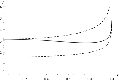
The function $\mathbf{t}(\lambda)$ deserves to be studied in some detail. One can see from its definition $(\ref{ttC1})$–$(\ref{ttC5})$ that the function $\mathbf{t}$ depends only on the elliptic coordinate $k$, i.e., only on the energy $E$ $(\ref{E})$ of pendulum $(\ref{ham_vert})$, but not on its phase $\varphi$. Thus we have a function

$$\mathbf{t}\,:\,E\mapsto\mathbf{t}(E),\qquad\mathbf{t}\,:\,[-1,+\infty)\to(0,+\infty].$$

Proposition 6.9.

• The function $\mathbf{t}(E)$ is smooth for $E\in[-1,1)\cup(1,+\infty)$.

• $\lim\limits_{E\to-1+0}\mathbf{t}(E)=\pi$; $\lim\limits_{E\to 1}\mathbf{t}(E)=+\infty$; $\mathbf{t}\sim 2\sqrt{2}\pi/\sqrt{E+1}\to 0$ as $E\to+\infty$.

Proof.

(1) follows from smoothness of the functions $K(k)$ and $p_{1}^{1}(k)$ for $k\in[0,1)$.

(2) follows from the limits $\lim\limits_{k\to+0}K(k)=\pi/2$, $\lim\limits_{k\to 1-0}K(k)=\lim\limits_{k\to 1-0}p_{1}^{1}(k)=+\infty$, $\lim\limits_{k\to 0}p_{1}^{1}(k)=2\pi$. ∎

A plot of the function $\mathbf{t}(E)$ is given at Fig. 9.

Figure 9: Plot of the function $E\mapsto\mathbf{t}(E)$

In our forthcoming work [19] we show that the inequality  $(\ref{tcut_bound_fin})$ is in fact an equality, i.e., $t_{\operatorname{cut}}(\lambda)=\mathbf{t}(\lambda)$ for $\lambda\in C$.

List of Figures

1. 1 Problem statement
2. 2 Decomposition of the cylinder $C$
3. 4.3 Parametrization of extremal trajectories
4. 5 Critical trajectory: $\lambda\in C_{3}$
5. 6 Reflections $\varepsilon^{i}\,:\,\delta\mapsto\delta^{i}$ of trajectories of pendulum
6. 7 Surfaces containing Maxwell strata $\operatorname{Max}\nolimits^{i}$
7. 8 Plots of the functions $K(k)\leq p_{1}^{1}(k)\leq 2K(k)$
8. 9 Plot of the function $E\mapsto\mathbf{t}(E)$

References

- [1] A. A. Agrachev, Exponential mappings for contact sub-Riemannian structures, Journal Dyn. and Control Systems 2(3), 1996, 321–358.
- [2] A.A. Agrachev, Geometry of optimal control problems and Hamiltonian systems, Springer, Lecture Notes in Mathematics, to appear.
- [3] A.A. Agrachev, Yu. L. Sachkov, Control Theory from the Geometric Viewpoint, Springer-Verlag, Berlin 2004.
- [4] C. El-Alaoui, J.P. Gauthier, I. Kupka, Small sub-Riemannian balls on , Journal Dyn. and Control Systems 2(3), 1996, 359–421.
- [5] U. Boscain, F. Rossi, Invariant Carnot-Caratheodory metrics on , , and Lens Spaces, SIAM J. Control Optim., to appear.
- [6] R. Brockett, Control theory and singular Riemannian geometry, In: New Directions in Applied Mathematics, (P. Hilton and G. Young eds.), Springer-Verlag, New York, 11–27.
- [7] J.P. Laumond, Nonholonomic motion planning for mobile robots, Lecture notes in Control and Information Sciences, 229. Springer, 1998.
- [8] O. Myasnichenko, Nilpotent (3,6) Sub-Riemannian Problem, J. Dynam. Control Systems 8 (2002), No. 4, 573–597.
- [9] O. Myasnichenko, Nilpotent sub-Riemannian problem, J. Dynam. Control Systems 8 (2006), No. 1, 87–95.
- [10] F. Monroy-Perez , A. Anzaldo-Meneses, The step-2 nilpotent sub-Riemannian geometry, J. Dynam. Control Systems, 12, No. 2, 185–216 (2006).
- [11] J.Petitot, The neurogeometry of pinwheels as a sub-Riemannian contact stucture, J. Physiology - Paris 97 (2003), 265–309.
- [12] L.S. Pontryagin, V.G. Boltyanskii, R.V. Gamkrelidze, E.F. Mishchenko, The mathematical theory of optimal processes, Wiley Interscience, 1962.
- [13] Yu. L. Sachkov, Exponential mapping in generalized Dido’s problem, Mat. Sbornik, 194 (2003), 9: 63–90 (in Russian). English translation in: Sbornik: Mathematics, 194 (2003).
- [14] Yu. L. Sachkov, Discrete symmetries in the generalized Dido problem (in Russian), Matem. Sbornik, 197 (2006), 2: 95–116. English translation in: Sbornik: Mathematics, 197 (2006), 2: 235–257.
- [15] Yu. L. Sachkov, The Maxwell set in the generalized Dido problem (in Russian), Matem. Sbornik, 197 (2006), 4: 123–150. English translation in: Sbornik: Mathematics, 197 (2006), 4: 595–621.
- [16] Yu. L. Sachkov, Complete description of the Maxwell strata in the generalized Dido problem (in Russian), Matem. Sbornik, 197 (2006), 6: 111–160. English translation in: Sbornik: Mathematics, 197 (2006), 6: 901–950.
- [17] Yu. L. Sachkov, Maxwell strata in Euler’s elastic problem, Journal of Dynamical and Control Systems, Vol. 14 (2008), No. 2 (April), pp. 169–234.
- [18] Yu. L. Sachkov, Conjugate points in Euler’s elastic problem, Journal of Dynamical and Control Systems, vol. 14 (2008), No. 3 (July), 409–439.
- [19] Yu. L. Sachkov, Cut time in sub-Riemannian problem on the group of motions of a plane, in preparation.
- [20] A.M. Vershik, V.Y. Gershkovich, Nonholonomic Dynamical Systems. Geometry of distributions and variational problems. (Russian) In: Itogi Nauki i Tekhniki: Sovremennye Problemy Matematiki, Fundamental’nyje Napravleniya, Vol. 16, VINITI, Moscow, 1987, 5–85. (English translation in: Encyclopedia of Math. Sci. 16, Dynamical Systems 7, Springer Verlag.)
- [21] E.T. Whittaker, G.N. Watson, A Course of Modern Analysis. An introduction to the general theory of infinite processes and of analytic functions; with an account of principal transcendental functions, Cambridge University Press, Cambridge 1996.