The quantum phase transition in the sub-ohmic spin-boson model:
Quantum Monte-Carlo study with a continuous imaginary time cluster algorithm

Abstract

A continuous time cluster algorithm for two-level systems coupled to a dissipative bosonic bath is presented and applied to the sub-ohmic spin-Boson model. When the power $s$ of the spectral function $J(\omega)\propto\omega^{s}$ is smaller than $1/2$, the critical exponents are found to be classical, mean-field like. Potential sources for the discrepancy with recent renormalization group predictions are traced back to the effect of a dangerously irrelevant variable.

Quantum-mechanical systems embedded into a dissipative environment play an important role in many areas of physics legget-etal ; weiss . Among the numerous applications of models that couple a small quantum-mechanical system to a bosonic bath are noisy quantum dots quantum-dots , decoherence of qubits in quantum computations qbits , and charge transfer in donor-acceptors systems transfer . A major research field are quantum impurity models (i.e. a quantum spin embedded in a crystal lattice, for a review see bulla-etal ), where in particular quantum critical points occurring for instance in the Bose-Fermi Kondo model have been studied intensively kevin ; kevin2 ; si ; si2 .

The paradigmatic model of a two-state system coupled to an infinite number of bosonic degrees of freedom is the spin-boson model legget-etal ; weiss . As a function of the strength of the coupling to its bath it displays a quantum phase transition (QPT) at zero temperature between a delocalized phase, which allows quantum mechanical tunneling between the two states, and a localized phase, in which the system ceases to tunnel in the low-energy limit and behaves essentially classically.

While the phase transition is understood in the case of ohmic dissipation ($s=1$), the sub-ohmic situation ($s<1$) has been investigated in detail only recently. On general grounds, one expects the phase transition to fall into the same universality class as that of the classical Ising spin chain with long-range interactions suzuki . Indeed, a continuous QPT has been found in the spin-boson model for all values of $0<s<1$ BTV , using a generalization of Wilson’s numerical renormalization group (NRG) technique bulla-etal . However, on the basis of these NRG calculations, it was suggested that the quantum-to-classical mapping fails for $s<1/2$ vojta : There, the Ising chain displays a mean-field transition, whereas the critical exponents extracted from NRG were non-mean-field-like and obeyed hyperscaling. Subsequent NRG calculations for the spin-boson karyn and Ising-symmetric Bose-Fermi Kondo model kevin confirmed this claim. Such a breakdown of quantum-to-classical mapping has consequences not only for quantum-dissipative systems, but also for Kondo lattice models studied within extended dynamical mean-field theory, where non-mean-field critical behavior is at the heart of so-called local quantum criticality si .

The purpose of this letter is two-fold: 1) We present a novel and accurate quantum Monte-Carlo (QMC) method to study the low temperature properties of the sub-ohmic spin-boson model, and 2) we determine its critical exponents at the quantum phase transition using this method together with finite temperature scaling and re-confirm the correctness of the quantum-classical mapping for the sub-ohmic bath with $s<1/2$.

The spin-boson Hamiltonian is defined as

$$H=\Delta\frac{\hat{\sigma}^{x}}{2}+\frac{\hat{\sigma}^{z}}{2}\,\sum_{i}\lambda_{i}({\bf a}_{i}+{\bf a}_{i}^{+})+\sum_{i}\omega_{i}\,{\bf a}_{i}^{+}{\bf a}_{i}$$ (1)

where $\sigma^{x,z}$ are Pauli spin-1/2 operators, ${\bf a}_{i}^{+}$, ${\bf a}_{i}$ are bosonic creation and annihilation operators, $\Delta$ the tunnel matrix element, and $\omega_{i}$ the oscillator frequencies of the bosonic degrees of freedom. The coupling between the the spin $\sigma$ and the bath via the $\lambda_{i}$ is determined by the spectral function for the bath:

$$J(\omega)=\pi\sum_{i}\lambda_{i}^{2}\delta(\omega-\omega_{i})=2\pi\alpha\cdot\omega_{c}^{1-s}\omega^{s}$$ (2)

for $0<\omega<\omega_{c}$ and $J(\omega)=0$ otherwise. $\alpha$ represents the coupling strength to the dissipative bath and $\omega_{c}$ is a cut-off frequency. The parameter $s$ specifies the low-frequency behavior of the spectral function: $s=1$ represents an ohmic bath, and $s<1$ a sub-ohmic bath. A system described by (1) and (2) displays for $s\leq 1$ a quantum phase transition (at zero temperature) at a critical coupling strength $\alpha_{c}$. In the following we determine the critical exponents and herewith the universality class of this transition with the help of a continuous time cluster algorithm that samples stochastically the imaginary time path integral for the partition function of the model (1).

Consider a Hamiltonian for an Ising spin in a transverse field of the form

$${\it H}=\Gamma\hat{\sigma}^{x}+{\it G}(\hat{\sigma}^{z},\underline{\hat{a}},\underline{{\omega}})\;,$$ (3)

where $\Gamma$ is the transverse field strength, $\Gamma=\Delta/2$ in (1), $\underline{\hat{a}}$ and $\underline{{\omega}}$ a set of Hermitian operators and parameters, respectively, like the Bose operators and coupling constants and frequencies in the spin-boson model. ${\it G}$ is a function of the $\hat{\sigma}^{z}$ and ($\underline{\hat{a}}$, $\underline{{\omega}}$) alone, it is Hermitian but otherwise arbitrary.

The partition function for this Hamiltonian is derived by implicitly performing the limit of an infinite number of time slices in its Suzuki-Trotter representation pich-etal ; rieger-kawa ; zamponi and yields the imaginary time path integral

$${\it Z} = {\rm Tr}_{\hat{\sigma},\underline{\hat{a}}}\exp(-\beta{\it H})$$ (4)

$$= \int{\it D}\sigma(\tau)\,\exp(-{\it S}_{\underline{{\omega}}}[\sigma(\tau)])$$ (5)

where ${\it S}_{\underline{{\omega}}}[\sigma(\tau)])=-\ln\,{\rm Tr}_{\underline{\hat{a}}}\exp[\int_{0}^{\beta}d\tau\,{\it G}(\sigma(\tau),\underline{\hat{a}},\underline{{\omega}})]$ and $\sigma(\tau)$ is now a real valued function of the imaginary time $\tau\in[0,\beta]$, denoted as a spin-1/2 world line. These world lines represent realizations of a two-valued Poissonian process that is sketched in Fig. 1a: They are piecewise constant functions consisting of consecutive segments of spin-up ($\sigma=+1$) and spin-down ($\sigma=-1$), where the spin-flips occur at stochastic times $0<\tau_{1}<\tau_{1},\ldots\tau_{n}$ ($n$ arbitrary) and the interval lengths $\Delta\tau_{i}=\tau_{i+1}-\tau_{i}$ obey a Poissonian statistics $P(\Delta\tau)=\Gamma^{-1}\exp(-\Gamma\Delta\tau)$ with mean value $1/\Gamma$ rieger-kawa . The path integral (5) can hence be directly sampled by generating stochastically realizations of such world lines and accepting them according to their “Boltzmann”-weight $\exp(-{\it S}_{\underline{{\omega}}}[\sigma(\tau)])$. More efficient sampling procedures like cluster algorithms are based on this principle rieger-kawa .

For a general transverse Ising model (without coupling to a dissipative bath) ${\it G}(\hat{\sigma}^{z})$ represents just the “classical” energy $E(\hat{\sigma}^{z})$ that is diagonal in the $z$-representation of the spin-1/2 degrees degrees of freedom and $S[\sigma(\tau)]=\int_{0}^{\beta}d\tau\,E(\sigma(\tau))$. This form holds for an arbitrary number of spins in a transverse field, and for arbitrary spin-spin interactions.

In the case of the spin-boson model (1) with the spectral function (2) the trace over the oscillator degrees of freedom yields weiss ${\it S}_{\underline{{\omega}}}={\it S}_{SB}$ with

$${\it S}_{SB}[\sigma(\tau)]=-\int_{0}^{\beta}d\tau\int_{0}^{\tau}d\tau^{\prime}\;\sigma(\tau)\,{\it K}_{\beta}(\tau-\tau^{\prime})\,\sigma(\tau^{\prime})\;.$$ (6)

The kernel imposes long-range interactions in imaginary time:

$${\it K}_{\beta}(\tau)=\int_{0}^{\infty}d\omega\,\,\frac{J(\omega)}{\pi}\frac{\cosh(\frac{\hbar\beta}{2}\omega[1-2\tau/\beta])}{\sinh(\frac{\hbar\beta}{2}\omega)}\;.$$ (7)

It has the symmetry ${\it K}(\beta-\tau)={\it K}(\tau)$ and the asymptotics ${\it K}(\tau)\propto\tau^{-(1+s)}$ for $\tau_{c}\ll\tau\ll\beta$, where $\tau_{c}=2\pi/\omega_{c}$. For $\tau<\tau_{c}$ the Kernel $K(\tau)$ is regularized via the frequency cut-off $\omega_{c}$ in (2) and approaches a constant for $\tau\to 0$.

An efficient way of sampling the path integral is a cluster algorithm based on rieger-kawa . It is generalization of the Swendsen-Wang cluster algorithm swendsen-wang to continuous time world lines, in which not individual spins but the world line segments are connected during the cluster-forming procedure, and has to incorporate the long-range interactions luijten . It is sketched in Fig. 1b: Starting from a world line configuration $\sigma(\tau)$ new potential spin-flip sites are introduced according to a Poissonian statistics, then all segments are pairwise “connected” with probability

$$p(s_{I},s_{II})=1-\exp\left(-2\,\int_{a}^{b}d\tau\int_{c}^{d}d\tau^{\prime}\,{\it K}_{\beta}(\tau-\tau^{\prime})\right)\;.$$ (8)

where $a,b$ and $c,d$ denote the limits of segment $S_{I}$ and $S_{II}$, respectively. Finally the connected clusters are identified and flipped with probability 1/2. All potential spin-flip times that do not represent real spin-flips are then removed.

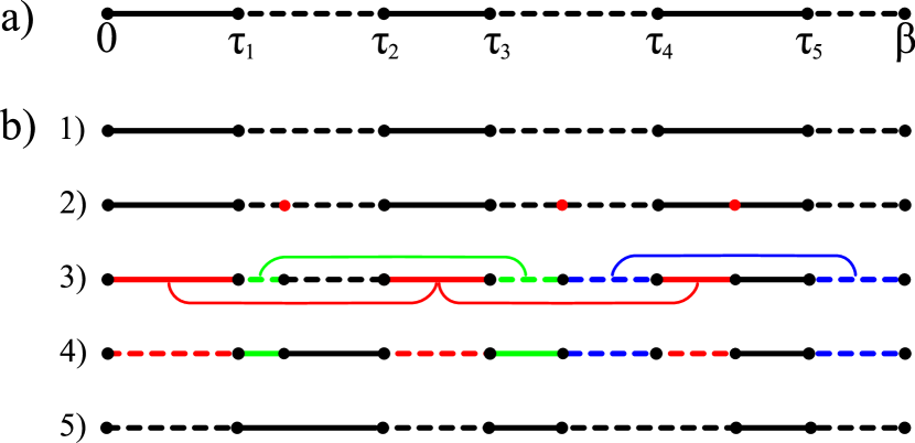
Figure 1: (Color online) a Realization of an imaginary time world line of a spin-1/2 in a transverse field. b) Sketch of the continuous time cluster update: 1) Starting configuration. 2) Random insertion of new potential spin flips (red dots) with Poissonian statistics 3) Connection of segments with probabilities given by eq.(8). Different colors indicate the resulting clusters. 4) Each cluster is flipped with probability 1/2 (the blue one was not flipped). 5) Resulting new imaginary time world line.

We implemented this algorithm and tested it by comparing results with those obtained with conventional Monte-Carlo procedures in discrete imaginary time extrapolated to an infinite number of time-slices. We analyzed the sampling characteristics of the algorithm for the kernel (7) with (2) over the whole range $0<s<1$ and found that on average after 5 updates as sketched in Fig.1b the world line configuration are statistically independent from the starting configuration. The data presented below represent averages over $10^{5}$-$10^{6}$ cluster updates.

To study the phase transition in the sub-ohmic spin-boson model ($s<0.5$) we utilize the finite-$\beta$ scaling forms for thermodynamic observables close to the critical point $\alpha=\alpha_{c}$

$$\langle{\it O}\rangle_{T,\alpha}=\beta^{x_{\it O}}g_{\it O}(\beta^{y_{t}^{*}}\delta)\;,$$ (9)

where $\delta=(\alpha-\alpha_{c})/\alpha_{c}$ denotes the distance from the critical point, $x_{\it O}$ and $g_{\it O}$ are the scaling exponent and scaling function of the observable ${\it O}$, respectively. The exponent $y_{t}^{*}$ is $1/\nu$ below the upper critical dimension ($s>1/2$), $\nu$ being the correlation length exponent, and $y_{t}^{*}=1/\nu+(1/2-s)$ above the upper critical dimension ($s<1/2$). luijten .

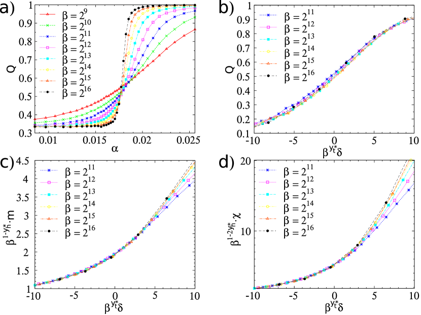
Figure 2: Results for the spin boson model for $s=0.2$ and $\Delta=0.1$. a) Moment-ratio $Q$ as a function of the coupling constant $\alpha$ for different values of $\beta$. The critical coupling is at $\alpha_{c}=0.0175\pm 0.0002$. b-c) Finite $\beta$-scaling for the moment-ratio $Q$, magnetization $m$ and susceptibility $\chi$ ($\delta=(\alpha-\alpha_{c})/\alpha_{c}$, with $\alpha_{c}$ from a). The values for the critical exponents are $y_{t}^{*}=0.5$, $y_{h}^{*}=0.75$. For large positive values of the scaling variable corrections to scaling are stronger.

We use the dimensionless ratio of moments $Q=\langle m^{2}\rangle^{2}/\langle m^{4}\rangle$, which has $x_{Q}=0$ and is therefore asymptotically independent of temperature at $\delta=0$, to locate the critical point $\alpha_{c}$ as shown for $s=0.2$ in Fig.2a. This estimate for $\alpha_{c}$ is then used to perform the finite-$\beta$ scaling analysis for $Q$, $Q=\tilde{Q}(\beta^{y_{t}^{*}}\delta)$ the magnetization $m=\langle|m|\rangle=\beta^{y_{h}^{*}-1}\tilde{m}(\beta^{y_{t}^{*}}\delta)$ and the susceptibility $\chi=\beta\langle m^{2}\rangle=\beta^{2y_{h}^{*}-1}\tilde{\chi}(\beta^{y_{t}^{*}}\delta)$, where $y_{h}^{*}$ is the magnetic exponent. The data collapse that one obtains with the mean-field values for the exponents $y_{t}^{*}$ and $y_{h}^{*}$

$$y_{t}^{*}=1/2\,,\quad y_{h}^{*}=3/4$$ (10)

is good, as shown Fig.2b-d.

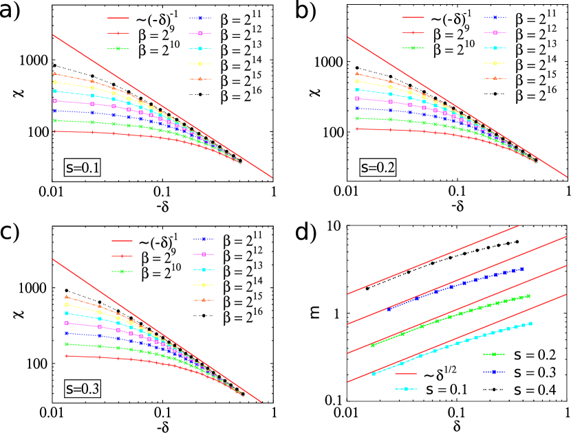
Figure 3: a-c) Data for the susceptibility $\chi$ as a function of the distance from the critical point $\delta>0$ (i.e. in the delocalized phase) for $s=0.1$ (a), $s=0.2$ (b) and $s=0.3$ for different values of $\beta$ ($\Delta$ and $\omega_{c}$ as in Fig.2). For increasing inverse temperature $\beta$ the data points approach the straight line, which is the zero temperature behavior $\chi\propto\delta^{-1}$. d) Magnetization $m$ as a function of $\delta>0$ (i.e. in the localized phase) for $\beta=2^{16}$ for different values of $s$ (multiplied with $2$, $4$ and $8$ for $s=0.2$, $s=0.3$ and $s=0.4$, respectively, for better visibility) The straight lines are guides for the eye proportional to the zero temperature behavior $(\alpha-\alpha_{c})^{-1/2}$. Shown are only the data that are free from finite-$\beta$ corrections.

At the critical point $\alpha=\alpha_{c}$ the scaling forms predict $\chi\propto T^{-x}$ with $x=2y_{h}^{*}-1=1/2$, which is clearly confirmed by our data displayed in Fig.2d: $\chi\cdot T^{1/2}$ collpaes onto one point at $\delta=0$. Moreover the scaling forms imply at $T=0$ $\chi\propto|\alpha-\alpha_{c}|^{-\gamma}$ with $\gamma=(2y_{h}^{*}-1)/y_{t}^{*}=1$, which is demonstrated in Fig.3a-c for different values of $s<1/2$., and $m\propto(\alpha-\alpha_{c})^{\beta_{m}}$ for $\alpha>\alpha_{c}$ with $\beta_{m}=-(y_{h}^{*}-1)/y_{t}^{*}=1/2$, which is demonstrated in Fig.3d.

Next we allow for an unbiased fit of the critical exponents to our data, including corrections to scaling as in luijten . We determined $y_{t}^{*}$ and $y_{h}^{*}$ by finite-$\beta$ scaling of $\partial Q/\partial\alpha\,(\alpha=\alpha_{c})\propto\beta^{y_{t}^{*}}$ and $\chi(\alpha=\alpha_{c})\propto\beta^{2y_{h}^{*}-1}$. The results confirm (10) within the error bars for the whole range of $s<1/2$ that we studied. Only close to $s=1/2$ the finite-$\beta$ scaling analysis is impeded by the presence of logarithmic corrections at the upper critical dimension. Fig.4a-b shows the resulting estimates for the exponents $1/\nu=y_{t}^{*}-(1/2-s)$ and $\beta_{m}=-(y_{h}^{*}-1)/y_{t}^{*}$ as a function of $s$ in comparison with the NRG predictions of vojta .

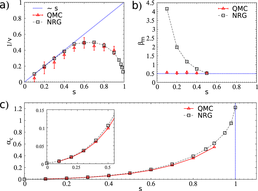
Figure 4: a-b) Numerical estimates of the critical exponents $1/\nu$ and $\beta_{m}$ as a function of $s$. Triangles: QMC result (obtained from finite temperature scaling of the QMC data as described in the text); squares: RG results (from vojta , compare also kevin ); straight lines: mean-filed values for $s<1/2$. c) Critical coupling strength $\alpha_{c}$ as a function of $s$ diagram for the spin-boson model (1-2) with cut-off frequency $\omega_{c}=1$ and tunnel matrix element $\Delta=0.1$. Triangles: QMC result; squares: NRG results for fixed NRG discretization parameter $\Lambda=2$ (from BTV ). Performing the limit $\Lambda\to 1$ moves the NRG-estimates for $\alpha_{c}$ slighlty downward.

Although our results for the critical exponents of the sub-ohmic bath obtained with our continuous imaginary time algorithm deviate from the NRG prediction, results for the phase diagram match: In Fig.4c our estimates for the critical coupling $\alpha_{c}$ are compared with those obtained with the NRG method vojta , they agree very well.

We confirmed the scenario described here for other values of $\Delta$ and $\omega_{c}$, and also for smooth frequency cut-offs as well as for other kernels (7), like one that has a regularization in time (${\it K}(\tau)=0$ for $\tau<\tau_{c}$) rather than in frequency. We also found that the limit $\omega_{c}\to\infty$ (or $\tau_{c}\to 0$) exists and is approached smoothly and fast, and conclude that, concerning the critical exponents, the regularization does not play a significant role.

We also implemented a conventional QMC algorithm in discrete time (with a finite number of Trotter time slices $M$) and found that for any fixed value of $\Delta\tau=\beta/M$ mean-field exponents describe perfectly the scaling at the critical point for $s<1/2$ (see also luijten ; remark ). Moreover we found that the extrapolation $M\to\infty$ of numerical data for $Q$, $m$ and $\chi$ obtained for fixed $M$ reproduces perfectly the results obtained with our continuous imaginary time cluster algorithm and that the convergence is smooth and fast (with $1/M$, as expected).

Our conclusion therefore is that the quantum-to-classical mapping does not fail in the sub-ohmic spin-Boson model. The question remains, why the NRG calculation presented in BTV ; vojta yields apparently correct results for quantities like the critical coupling, i.e. the phase diagram (see Fig. 4c), but fails to predict the correct critical exponents in the case $s<1/2$.

We believe the problem is rooted in a shortcoming of the present NRG implementation. As detailed in Ref. BLTV, , due to the truncation of the bosonic Hilbert space, the NRG – while correctly describing the delocalized phase and the critical point – it is unable to capture the physics of localized phase of the spin-boson model for $s<1$. Technically, a finite expectation value $\langle\sigma_{z}\rangle$ is accompanied by a mean shift of the bath oscillators which diverges in the low-energy limit. Hence, the NRG results are expected to be reliable as far as they do not involve properties of the localized fixed point.

The analysis of critical exponents in Ref. vojta, now assumed that all exponents are properties of the critical fixed point. However, this assumption is invalid for the order-parameter related exponents $\beta_{m}$ and $\delta_{m}$ if the critical fixed point is Gaussian (like in a $\phi^{4}$ theory above its upper critical dimension). Then, the order parameter amplitude is controlled by a dangerously irrelevant variable, and $\beta_{m}$ and $\delta_{m}$ are properties of the flow towards the localized fixed point, which in turn is not correctly captured by NRG. (Note that $\delta_{m}$ involves the non-linear field response at criticality, which is undefined for a purely Gaussian theory.) Therefore, the values of $\beta_{m}$ and $\delta_{m}$ extracted from (present) NRG calculations are unreliable.

Considering that the NRG calculations nevertheless gave well-defined power laws which were moreover consistent with hyperscaling, it is worth asking for the underlying reason. We conjecture that the artificial Hilbert-space truncation, which determines the flow to the “wrong” localized fixed point and limits both the field response and the condensate amplitude, is equivalent to an operator which is exactly marginal at criticality in the $\phi^{4}$ language. Near criticality, this has no consequences below the upper critical dimension, $s>1/2$, as the quartic interaction is relevant here, but for $s<1/2$ the marginal operator instead dominates over the quartic term. It is easy to show that an exactly marginal coupling leads to $y_{h}^{*}=(1+s)/2-y_{i}$ with $y_{i}=0$ such that hyperscaling is fulfilled, while $y_{t}^{*}$ takes its mean-field value – this is what characterizes the set of NRG critical exponents vojta . (The correct result $y_{h}^{*}=3/4$ for $s<1/2$ implies $y_{i}=(2s-1)/4$ arising from the dangerously irrelevant variable.) The above reasoning is supported by analyzing fermionic impurity models, which naturally have the property that a Hilbert space constraint limits the field response. For instance, a resonant-level model with power-law bath density of states, which is controlled by a stable intermediate-coupling fixed point, shows hyperscaling for all bath exponents LFMV .

Finally, the analytical RG argument in Ref. vojta, , based on an epsilon-expansion for small $s$, predicted non-mean-field exponents obeying hyperscaling for a related reason: While the RG equations (9)-(11) of Ref. vojta, are correct, the subsequent analysis overlooked the presence of the dangerously irrelevant variable, resulting again in the incorrect $y_{h}^{*}=(1+s)/2$.

To conclude we have, with the help of an efficient and accurate continuous time cluster Monte-Carlo algorithm, shown that the quantum-to-classical mapping is valid in the case of the sub-ohmic spin-boson model. The presence of a dangerously irrelevant variable for $s<1/2$ impedes the correct extraction of the critical exponents with current versions of the NRG method - work on its extension to produce reliably the necessary determination of magnetic observables in the localized phase is in progress.

References

- (1) A. J. Leggett, et al. Rev. Mod. Phys. 59, 1 (1987).
- (2) U. Weiss, Quantum Dissipative Systems (World Scientific, Singapore, 1999).
- (3) K. Le Hur, Phys. Rev. Lett. 92, 196804 (2004); M. R. Li, K. Le Hur, W. Hofstetter, Phys. Rev. Lett. 95, 086406 (2005).
- (4) M. Thorwart, P. Hänggi, Phys. Rev. A 65, 012309 (2001); T. A. Costi, R. H. McKenzie, Phys. Rev. A 68, 034301 (2003).
- (5) S. Tornow, N.H. Tong, R. Bulla, Europhys. Lett. 73, 913 (2006).
- (6) R. Bulla, T. A. Costi, T. Pruschke, Rev. Mod. Phys. 80, 395 (2008).
- (7) M. T. Glossop and K. Ingersent, Phys. Rev. Lett. 95, 067202 (2005); Phys. Rev. B 75, 104410 (2007).
- (8) M. T. Glossop and K. Ingersent, Phys. Rev. Lett. 99, 227203 (2007).
- (9) Q. Si, S. Rabello, K. Ingersent, and J. L. Smith, Nature (London) 413, 804 (2001); Phys. Rev. B 68, 115103 (2003).
- (10) L. Zhu, S. Kirchner, Q. Si, A. Georges, Phys. Rev. Lett. 93, 267201 (2004); J.-X. Zhu, S. Kirchner, R. Bulla, Q. Si, Phys. Rev. Lett. 99, 227204 (2007); S. Kirchner, Q. Si, Phys. Rev. Lett. 100, 026403 (2008).
- (11) M. Suzuki, Progr. Theor. Phys. 56, 1454 (1976).
- (12) R. Bulla, N.H. Tong, and M. Vojta, Phys. Rev. Lett. 91, 170601 (2003).
- (13) M. Vojta, N.H. Tong, and R. Bulla, Phys. Rev. Lett. 94, 070604 (2005).
- (14) K. Le Hur, P. Doucet-Beaupre, and W. Hofstetter, Phys. Rev. Lett. 99, 126801 (2007).
- (15) C. Pich, A. P. Young, H. Rieger, N. Kawashima, Phys. Rev. Lett. 81, 5916 (1998).
- (16) H. Rieger, N. Kawashima, Europ. Phys. J. B 9, 233 (1999).
- (17) F. Krzakala, A. Rosso, G. Semerjian, F. Zamponi, arXiv:0807.2553.
- (18) R.H. Swendsen, J.-S. Wang, Phys. Rev. Lett. 58, 86 (1987).
- (19) E. Luijten, H. W. J. Blöte, Phys. Rev. B 56, 8945 (1997).
- (20) M. Troyer (private comminication); S. Kircher and Q. Si (unpublished).
- (21) R. Bulla, H.-J. Lee, N.H. Tong, and M. Vojta, Phys. Rev. B 71, 045122 (2005).
- (22) L. Fritz and M. Vojta, Phys. Rev. B 70, 214427 (2004).