The ice-limit of Coulomb gauge Yang-Mills theory

Abstract

In this paper we describe gauge invariant multi-quark states generalising the path integral framework developed by Parrinello, Jona-Lasinio and Zwanziger to amend the Faddeev-Popov approach. This allows us to produce states such that, in a limit which we call the ice-limit, fermions are dressed with glue exclusively from the fundamental modular region associated with Coulomb gauge. The limit can be taken analytically without difficulties, avoiding the Gribov problem. This is illustrated by an unambiguous construction of gauge invariant mesonic states for which we simulate the static quark–antiquark potential.

1 Introduction

Yang-Mills theories are the cornerstone of the standard model. Their success is largely based upon perturbation theory where gauge fixing, implemented using the Faddeev-Popov method [1], plays a key role. However, Gribov [2] has pointed out that, at a non-perturbative level, the Faddeev-Popov method fails since there are always gauge equivalent (Gribov) copies which satisfy a chosen gauge condition. Initially this was shown for Coulomb gauge, but Singer has proven that this is in fact a general problem [3].

There have been various attempts to extend the Faddeev-Popov method to the non-perturbative regime. For example, it was suggested that the various Gribov copies, weighted by the Faddeev-Popov determinant, should contribute to the functional integral with alternating signs. This approach can be viewed as the insertion of a topological invariant into the partition function. Unfortunately, that topological invariant turns out to be zero in SU($N_{c}$) Yang-Mills theory leaving us with the disastrous conclusion that the generalised Faddeev-Popov method results in physical observables being in indeterminate form [4, 5, 6].

This state of affairs is unfortunate as the need for non-perturbative gauge fixing is widely recognised as physically desirable. For example, Dyson-Schwinger equations are widely used in hadron phenomenology, and their construction relies on unambiguous gauge fixing, in particular in the infra-red regime. Using stochastic quantisation to by-pass the Gribov problem [7, 8, 9], Zwanziger showed [10] that the tower of Dyson-Schwinger equations is unchanged but supplemented with additional constraints reflecting that gauge configurations are confined to the first Gribov region. It turns out that the Green’s functions solving the Dyson-Schwinger equations [11, 12, 13] appear to agree to a large extent with lattice simulations [14, 15, 16]. We note, however, that some initial discrepancies [17, 18, 19] in the infra-red [20] behaviour of Green’s functions have been confirmed in large volume simulations [21, 22]. It became clear only recently that these findings can be accommodated by the Gribov-Zwanziger approach when the Gribov-Zwanziger action is appropriately modified while preserving renormalisability and BRST invariance [23, 24].

To go beyond the Faddeev-Popov method, we will here use an alternative construction of the partition function [25, 26] which defines a gauge invariant action by integrating a weight function over the gauge orbit. This method has been studied on the lattice in the strong coupling expansion [27, 28], and in numerical simulations of the weak-coupling regime [29]. The phase diagram was explored in [30], and a phase transition from the weak to the strong gauge fixing regime was reported. Finally, it was argued in [31] that the gluon propagator displays gluon confinement. As we shall show, in a particular limit, which we call the ice-limit, the weight function constrains the gauge configurations to unique representatives of each gauge orbit. Altogether, these form what is called the fundamental modular region.

In a Hamiltonian framework integration over the gauge group may be used to define projection operators onto the different non-Abelian charge (superselection) sectors of the Yang-Mills Hilbert space in the presence of external charges. This was first emphasised by Polyakov [32] and Susskind [33] and subsequently worked out in detail by a number of authors (see e.g. [34, 35]). More recently Zarembo has used this approach to discuss the Yang-Mills mass gap, confinement and the interquark potential [36, 37] (see also [38, 39]). A thorough study of U(1) quantum mechanics along these lines may be found in [40].

In this paper, we introduce gauge invariant external fields (such as heavy quarks) through the projection techniques [32, 33, 34, 35, 36, 37] into the above alternative construction of the partition function [25, 26]. Using lattice regularisation, we will study the ice-limit where the fields are restricted to the fundamental modular region of Coulomb gauge. As an illustration, we will calculate the static heavy quark–antiquark potential.

2 Non-perturbative gauge fixing

2.1 The Gribov problem

Recall that gauge fixing amounts to identifying the space $\mathfrak{A}/\mathfrak{G}$ of gauge inequivalent configurations (that is the space $\mathfrak{A}$ of all configurations $A$ modulo gauge transformations $g\in\mathfrak{G}$) with a subset of the total configuration space: $\mathfrak{A}/\mathfrak{G}\subset\mathfrak{A}$. The original idea of gauge fixing (due to Weyl, see [41] for the historical context) attempts at choosing a gauge ‘slice’ $\Gamma$ (of configurations satisfying the gauge condition) to be identified with the physical configuration space. While this works for the Abelian case, it fails for the non-Abelian theory due to the existence of residual gauge copies, as shown by Gribov [2], who was also the first to suggest a possible solution. As the copies only appear as one moves away from the perturbative small field regime and reaches what is called the ‘Gribov horizon’ it seems appropriate to just stay within its interior, i.e. within the Gribov region. Mathematically, this is defined as that neighbourhood of the classical vacuum ($A=0$) where the Faddeev-Popov operator has a positive spectrum. It turns out, however, that this ‘off-limits’ prescription is not sufficient. Let us briefly recapitulate the problem and its (formal) solution.

Following ‘t Hooft [42] one may formulate the gauge fixing procedure in terms of distance functionals $S_{\mathrm{fix}}[A^{g}]\equiv\|A^{g}\|^{2}$ with $\|\;.\;\|^{2}$ an appropriate $L^{2}$ norm. As shown by Semenov-Tyan-Shanskii and Franke [43] as well as dell’Antonio and Zwanziger [44] the extrema of $S_{\mathrm{fix}}$ define the gauge condition while its Hessian (at the critical points) is the Faddeev-Popov operator such that the Gribov region is the domain of positive curvature containing $A=0$, known to be convex and to cover all orbits [43, 44]. Its boundary is the Gribov horizon where the lowest eigenvalue of the Faddeev-Popov operator vanishes. These authors also realised that there are copies remaining within the Gribov region, and one has to restrict configurations even further to the set $\Lambda$ of global minima,

$$\Lambda\equiv\{A\in\mathfrak{A}:S_{\mathrm{fix}}[A]\leq S_{\mathrm{fix}}[A^{g}],\;\mbox{for all}\;g\in\mathfrak{G}\}\;.$$ (1)

Note that, by construction, this set is included in the Gribov region and hence the gauge slice. As pointed out by van Baal [45] one still requires suitable boundary identifications within $\partial\Lambda$ endowing the subset $\Lambda\subset\mathfrak{A}$ with the appropriate topology before it can finally be identified with the physical configuration space of gauge inequivalent configurations. In this context the latter is denoted the fundamental modular region (FMR), see [46, 47] for reviews on this subject. We emphasise at this point that it is gauge invariant by construction. The details of the embedding $\mathfrak{A}/\mathfrak{G}\subset\mathfrak{A}$, however, will depend on the gauge fixing (functional) chosen as its starting point.

2.2 An alternative implementation of gauge fixing

As we have discussed, a gauge fixing condition $\chi_{a}[A]=0$ can always be identified as a stationary point of a gauge fixing functional $S_{\mathrm{fix}}[A^{g}]$ such that

$$\frac{\delta}{\delta\theta^{a}(x)}\,S_{\mathrm{fix}}[A^{g}]=0\implies\chi_{a}[A]=0\;,$$ (2)

where the fields $\theta^{a}(x)$ parameterise the gauge transformation, $g(x)=\exp\{i\theta^{a}(x)\,t^{a}\}$, with $t^{a}$ being the generator of the SU($N_{c}$) gauge group. The Faddeev-Popov approach is then based on the usual assumption [48, Chapter 16] that one can write 1 as

$$1=\int\!\mathcal{D}\theta\ \delta(\chi_{a}[A^{g}])\ \hbox{Det}\bigg{(}\frac{\delta\chi[A^{g}]}{\delta\theta}\bigg{)}\;\;.$$ (3)

This, though, is not true non-perturbatively (see Appendix A for more details) as, in fact, the right hand side of (3) is zero. We will therefore use a different approach here [25, 26], and, after reviewing it, we will study a series of examples.

The starting point of this approach is the definition of a gauge invariant effective action $S_{\mathrm{eff}}[A]$ derived from the gauge fixing functional via the identity

$$1=\mathrm{e}^{-S_{\mathrm{eff}}[A]}\int{\cal D}g\;\mathrm{e}^{S_{\mathrm{fix}}[A^{g}]},$$ (4)

where ${\cal D}g$ is the Haar measure on the gauge group. As it stands, this is a purely formal definition and one might ask if the right hand side of (4) is genuinely 1. In the continuum this question is hard to address, but using a lattice regulator it becomes clear that this really is a 1. To this end, we need to translate into a lattice formulation where the potential $A_{\mu}(x)$ is replaced by link variables $U_{\mu}(x)$ which transform under a gauge transformation (now conventionally written as $\Omega(x)$) according to

$$U_{\mu}^{\Omega}(x)=\Omega(x)U_{\mu}(x)\Omega^{\dagger}(x+ae_{\mu})\,.$$ (5)

Inserting (4) into the Yang-Mills partition function we obtain

$$Z=\int{\cal D}U_{\mu}\,{\cal D}\Omega\;\mathrm{e}^{S_{\mathrm{fix}}[U^{\Omega}]}\,\mathrm{e}^{-S_{\mathrm{eff}}[U]}\,\mathrm{e}^{S_{\mathrm{YM}}[U]}\;.$$ (6)

For such a lattice regulated partition function, we may interchange the integration over the links $U_{\mu}$ and the gauge transformations $\Omega$:

$$Z = \int{\cal D}\Omega\,{\cal D}U_{\mu}\;\mathrm{e}^{S_{\mathrm{fix}}[U^{\Omega}]}\,\mathrm{e}^{-S_{\mathrm{eff}}[U]}\,\mathrm{e}^{S_{\mathrm{YM}}[U]}=\int{\cal D}\Omega\,{\cal D}U^{\Omega}_{\mu}\;\mathrm{e}^{S_{\mathrm{fix}}[U^{\Omega}]}\,\mathrm{e}^{-S_{\mathrm{eff}}[U^{\Omega}]}\,\mathrm{e}^{S_{\mathrm{YM}}[U^{\Omega}]}$$ (7)

$$= \left(\int{\cal D}\Omega\right)\;\int{\cal D}U_{\mu}\,\mathrm{e}^{S_{\mathrm{fix}}[U]}\,\mathrm{e}^{-S_{\mathrm{eff}}[U]}\,\mathrm{e}^{S_{\mathrm{YM}}[U]},$$

from the invariance of the action and the Haar measure. This means that we have been able to factor out the gauge redundancies into a volume factor in much the same way as the original Faddeev-Popov trick tried to do. However, as we shall see, this procedure is valid non-perturbatively.

We will now investigate how this construction is used in three examples.

2.3 Three examples

2.3.1 The Christ-Lee Model

The Christ–Lee partition function [49] is given by the two dimensional integral

$$Z_{{}_{\text{CL}}}=\int d^{2}x\;\mathrm{e}^{S_{{}_{\mathrm{CL}}}(\boldsymbol{x})},$$ (8)

where $S_{{}_{\text{CL}}}(\boldsymbol{x})$ is a function depending only on $r\equiv\sqrt{x^{2}+y^{2}}$. Gauge transformations are rotations through an angle $\phi$, which we write $\boldsymbol{x}\to\boldsymbol{x}^{\,\phi}$. Taking, for example, $S_{{}_{\text{CL}}}(\boldsymbol{x})=-\boldsymbol{x}^{\,2}$, one may check that $Z_{{}_{\text{CL}}}=2\pi\times 1/2$, where the $2\pi$ comes from the integral over the angle $\phi$ and $1/2$ is the ‘physical’ partition function. We will consider the following gauge fixing functional

$$S_{\text{fix}}[\boldsymbol{x}^{\phi}]=-\frac{\kappa}{2}\left(\boldsymbol{x}^{\phi}-\boldsymbol{v}\right)^{2}\;,$$ (9)

where $\boldsymbol{v}$ is an external “gauge fixing” vector. The corresponding gauge condition

$$\frac{\partial S_{\mathrm{fix}}[\boldsymbol{x}^{\phi}]}{\partial\phi}=0\implies\boldsymbol{v}\cdot\boldsymbol{x}^{\,\phi+\pi/2}=0\;,$$

exhibits two Gribov copies: $\boldsymbol{x}^{\phi}$ parallel or antiparallel to $\boldsymbol{v}$. The FMR is given by those vectors $\boldsymbol{x}$ which (globally) maximise the gauge fixing action. In the present case, these are all vectors of arbitrary length parallel to $\boldsymbol{v}$. Without loss of generality, we choose $\boldsymbol{v}=(1,0)$ so that the gauge fixing condition becomes $y=0$. The FMR is then given by the positive $x$–axis (with Gribov copies appearing on the negative $x$–axis).

In analogy to (4), we find an effective action

$$\exp\big{(}S_{\text{eff}}[\boldsymbol{x}]\big{)}=\int\!\mathrm{d}\phi\ \exp\big{(}S_{\mathrm{fix}}[\boldsymbol{x}^{\phi}]\big{)}=2\pi I_{0}(\kappa r)\,\exp\bigg{(}-\frac{\kappa}{2}\,r^{2}-\frac{\kappa}{2}\bigg{)}\;,$$ (10)

with $I_{0}$ a modified Bessel function of the first kind. The effective action is manifestly gauge invariant as it depends only on $r$. We now insert the associated representation of unity,

$$\begin{split}1&=\exp\big{(}-S_{\text{eff}}[\boldsymbol{x}]\big{)}\int\!\mathrm{d}\phi\ \exp\big{(}S_{\mathrm{fix}}[\boldsymbol{x}^{\phi}]\big{)}\\ &=\frac{1}{2\pi\,I_{0}(\kappa r)}\int\!\mathrm{d}\phi\ \exp\big{(}\,\kappa\,\boldsymbol{x}^{\phi}\cdot\boldsymbol{v}\,\big{)}\;,\end{split}$$ (11)

into the partition function (8) where it follows from the discussion in Section 2.2 that

$$Z_{{}_{\text{CL}}}=\left(\int\!\mathrm{d}\phi\right)\,\int\!\mathrm{d}^{2}x\ \exp\big{(}S_{{}_{\mathrm{CL}}}(x)\big{)}\frac{e^{\,\kappa\,x}}{2\pi\,I_{0}(\kappa r)}\;,$$ (12)

using $\boldsymbol{x}\cdot\boldsymbol{v}=x$. For $S_{{}_{\text{CL}}}=-|\boldsymbol{x}|^{2}$, it is a straightforward matter to perform the $\mathrm{d}^{2}x$ integral in (12) and show that we recover the expected value of $1/2$. The important point is that the Gribov problem does not hamper this calculation. This can be made explicit by considering the limit of large $\kappa$, where the asymptotic behaviour of the modified Bessel function gives

$$Z_{\text{CL}}\simeq\left(\int d\phi\right)\,\int d^{2}x\;\mathrm{e}^{S_{\mathrm{CL}}(x)}\,\sqrt{\frac{\kappa\,r}{2\pi}}\,\mathrm{e}^{-\kappa\,(r-x)}\;.$$ (13)

Importantly, $\kappa(r-x)>0$ so that the $\kappa$ dependent terms of (13) are a Gaussian regularisation of the delta function. The support of the delta function arising in the $\kappa\to\infty$ limit are those vectors $\boldsymbol{x}$ for which

$$\kappa(r-x)=0\qquad\implies\qquad y=0\quad\text{and}\quad x\geq 0.$$

The condition $y=0$ corresponds to our chosen gauge condition, but the condition $x\geq 0$ restricts us to only the FMR, i.e. the Gribov copy at $x<0$ is not seen by the partition function. Explicitly:

$$\lim_{\kappa\to\infty}\sqrt{\frac{\kappa\,r}{2\pi}}\ \mathrm{e}^{-\kappa(r-x)}=|x|\,\theta(x)\,\delta(y)\;,$$ (14)

where $\theta$ is the Heaviside step function. Using this in (13) our final result for the $\kappa\to\infty$ limit is:

$$Z_{{}_{\text{CL}}}=\bigg{(}\int\!\mathrm{d}\phi\bigg{)}\int\!\mathrm{d}^{2}x\ \mathrm{e}^{S_{\mathrm{CL}}(x)}\,\theta(x)\;|x|\;\delta(y),$$ (15)

Our approach has not only correctly produced the gauge fixing constraint in terms of the $\delta$ function and the Faddeev–Popov determinant $|x|$, but also the correct “horizon function” [50, 51] $\theta(x)$, which singles out the FMR to the right of the Gribov horizon at $x=0$.

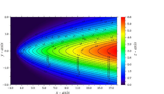
Figure 1: Contour plots of the $\kappa$ dependent fraction in (12), at $\kappa=16$. The support of this combination of $S_{\text{eff}}$ and $S_{\text{fix}}$, and thus of the partition function $Z_{{}_{\text{CL}}}$, is restricted to the FMR at large $\kappa$.

In Figure 1 we give contour plots of the $\kappa$ dependent fraction in (12), at $\kappa=16$. We clearly see the FMR emerging as the domain of support. The discussion of a more general class of gauge fixing functions is left to Appendix B.

2.3.2 Example: U(1) Landau gauge

As a second example we consider U(1) gauge theory in Landau gauge. Although this does not have a traditional Gribov problem, zero-modes must be eliminated in order for the Faddeev-Popov determinant to be non-zero.

The gauge fields $A_{\mu}(x)$ change under gauge transformations as

$$\Omega(x)=\mathrm{e}^{i\lambda(x)}\;,\hbox to28.45274pt{\hfill}A_{\mu}^{\Omega}(x)=A_{\mu}(x)+\partial_{\mu}\lambda(x)\;.$$ (16)

We choose Dirichlet boundary conditions:

$$A_{\mu}(x)|_{x\in\partial V}=0,\hbox to28.45274pt{\hfill}\lambda(x)|_{x\in\partial V}=\lambda_{0}$$ (17)

with $\lambda_{0}$ being constant. The gauge fixing action for Landau gauge is given by

$$S_{\text{fix}}[A]=-m^{2}\int\!\mathrm{d}^{4}x\ A_{\mu}A^{\mu}(x)\;,$$ (18)

where the “mass” $m$ acts as a gauge fixing parameter. This gauge fixing action generates the Landau gauge condition via

$$\frac{\delta}{\delta\lambda(x)}S_{\text{fix}}[A^{\lambda}]=0\implies\partial^{\mu}A^{\lambda}_{\mu}=0\;.$$ (19)

Given the boundary conditions (17), it follows that any $\lambda(x)$ may be written

$$\lambda(x)=\lambda_{0}+{\overline{\lambda}}(x)\;.$$ (20)

where $\lambda_{0}$ is the surface value of $\lambda(x)$ and $\overline{\lambda}(x)$ vanishes on $\partial V$ ($\overline{\lambda}$ may be decomposed as a sum over the non-zero Fourier modes of the Laplace operator). The measure on the algebra elements $\lambda$ is inherited from the group, so that $\mathcal{D}\Omega=\mathrm{d}\lambda_{0}\mathcal{D}\bar{\lambda}$. Note that the gauge fixing action (18) is invariant under constant gauge transformations since $A\to A+\partial\lambda=A+\partial\overline{\lambda}$. We must adopt some prescription to deal with the zero modes and to this end we will include in our measure a delta function $\delta(\lambda_{0})$ which kills the zero mode and makes the d’Alembertian $\square$ invertible. We are therefore led to propose the following form for the effective action:

$$e^{S_{\text{eff}}[A]}=\int\!\mathcal{D}\overline{\lambda}\ \exp\big{(}S_{\text{fix}}[A^{\overline{\lambda}}]\big{)}=\text{det}^{-1/2}(-m^{2}\square)\exp\big{(}-S_{\text{fix}}[A^{T}]\big{)}\;.$$ (21)

The transverse gauge field $A^{T}$ is defined by

$$A^{T}_{\mu}=\bigg{(}\eta_{\mu\nu}-\frac{1}{\square}\partial_{\mu}\partial_{\nu}\bigg{)}A^{\nu}\;,$$ (22)

and is gauge invariant. This result may be used in (7) to obtain the partition function of U(1) gauge theory. We evaluate

$$S_{\text{fix}}[A]-S_{\text{eff}}[A]=-m^{2}\int\!\mathrm{d}^{4}x\ A_{\mu}^{L}A^{L\mu}+\frac{1}{2}\log\text{det}(-m^{2}\square)\;,$$ (23)

where the longitudinal part of the field is defined by $A^{L}\equiv A-A^{T}$ . Inserting our representation of unity into the partition function we find that for this U(1) theory

$$Z=\text{det}^{-1/2}(-m^{2}\square)\ \int\!\mathcal{D}A_{\mu}\ \exp\big{(}-S_{\text{YM}}[A]-m^{2}\int\!\mathrm{d}^{4}x\ A^{L}_{\mu}A^{L\mu}\big{)}\;.$$ (24)

Note that the gauge fixing parameter $m$ acts as a mass for the longitudinal gauge fields. In the large mass limit, these decouple from the partition function leaving us with transverse fields only.

2.3.3 Example: SU(2) and weak gauge fixing

In our final example we consider SU(2) Yang-Mills theory, in lattice regularisation, with the gauge fixing functional

$$S_{\mathrm{fix}}[U^{\Omega}]=\kappa\sum_{x,\mu}\hbox{tr}U_{\mu}^{\Omega}(x),\hbox to28.45274pt{\hfill}\mu=1\ldots 4\;,$$ (25)

which implies (lattice) Landau gauge upon extremisation. When applied to the partition function $Z$, the (local) maxima of $S_{\text{fix}}$ give the dominant contributions at large $\kappa$. We refer to this as the ‘strong gauge fixing’ limit.

As we have illustrated with our previous models the use of the effective action approach is not limited to the large $\kappa$ regime. Here, we take $\kappa\ll 1$, the ‘weak gauge fixing’ limit, and calculate the effective action perturbatively in $\kappa$. Expanding the defining equation (4) and noting that $S_{\mathrm{fix}}$ is of order $\kappa$, we find, up to fourth order in $\kappa$,

$$S_{\mathrm{eff}}[U] = \frac{1}{2}\left\langle S^{2}_{\mathrm{fix}}\right\rangle\,+\,\frac{1}{24}\left[\left\langle S^{4}_{\mathrm{fix}}\right\rangle-3\left\langle S^{2}_{\mathrm{fix}}\right\rangle^{2}\right]+{\cal O}(\kappa^{6})\;,$$ (26)

$$\left\langle S^{n}_{\mathrm{fix}}\right\rangle := \int{\cal D}\Omega\;S^{n}_{\mathrm{fix}}[U^{\Omega}].$$ (27)

For SU(2), terms with an odd power of $\kappa$ vanish upon integration over $\Omega$. The term quadratic in $\kappa$ is independent of the links since there is no gauge invariant combination of two link variables apart from a constant:

$$\left\langle S^{2}_{\mathrm{fix}}\right\rangle=\frac{\kappa^{2}}{4}N_{l},$$ (28)

where $N_{l}$ is the number of links on the lattice. The calculation of the fourth order term is tedious but straightforward. We find:

$$\left\langle S^{4}_{\mathrm{fix}}\right\rangle-3\left\langle S^{2}_{\mathrm{fix}}\right\rangle^{2}=\frac{\kappa^{4}}{8}N_{l}+\frac{\kappa^{4}}{64}\sum_{p}\frac{1}{2}\hbox{tr}P_{p}[U],$$ (29)

where the sum extends over all plaquettes, $P_{p}$. Inserting (29) and (28) in (26), we finally obtain:

$$S_{\mathrm{eff}}[U]=N_{l}\left[\frac{1}{2}\left(\frac{\kappa}{2}\right)^{2}+\frac{1}{12}\left(\frac{\kappa}{2}\right)^{4}\right]+\frac{1}{4}\left(\frac{\kappa}{2}\right)^{4}\sum_{p}\frac{1}{2}\hbox{tr}P_{p}[U]+{\cal O}(\kappa^{6}).$$ (30)

For sufficiently small $\kappa$, the effect of $S_{\mathrm{eff}}[U]$ is just to correct the coefficient $\beta$ of the plaquette in the Wilson action, showing explicitly that $S_{\text{eff}}[U]$ is gauge invariant. Terms such as the $1\times 2$ Wilson loop appear at order $\kappa^{6}$.

3 Non-perturbative dressing

In this section we will introduce gauge invariant heavy quarks into the above approach to the partition function. We will adopt a Schrödinger representation, considering gauge invariant states constructed in a single time slice. Transition amplitudes between such states will be discussed in section 4. We begin by briefly reviewing the construction of gauge invariant charges [52].

A gauge invariant charged state $|\,Q\,\rangle$ may be constructed from a fermionic state $q(\boldsymbol{x})|\,0\,\rangle$ by ‘dressing’ the latter with an appropriate function $h[A]$ of the gauge field $A$,

$$|\,Q\,\rangle:=h[A](\boldsymbol{x})\,q(\boldsymbol{x})|\,q\,\rangle\;.$$ (31)

From the transformation properties of the fermion, $q(\boldsymbol{x})\to\Omega(\boldsymbol{x})q(\boldsymbol{x})$, requiring gauge invariance of the state $|\,Q\,\rangle$ implies that the dressing $h[A]$ transforms as

$$h^{\Omega}[A](\boldsymbol{x})=h[A](\boldsymbol{x})\,\Omega^{\dagger}(\boldsymbol{x})\;.$$ (32)

Dressings may be constructed through a field–dependent gauge transformation which rotates a given field $A$ into a gauge $\chi[A]=0$ . The dressing factor is not unique and should be selected according to its physical properties [53, 54]. For example, the dressing describing a single static quark in SU($N_{c}$) comes from the field dependent rotation into Coulomb gauge defined by

$$\partial_{i}\bigg{(}h\,A_{i}\,h^{-1}+ih\,\partial_{i}h^{-1}\bigg{)}=0\;.$$ (33)

From this example it is clear that the above dressing approach is sensitive to the Gribov problem of Coulomb gauge: although a gauge invariant charge may be constructed perturbatively from a solution of (33), Gribov copies imply that the dressing factor is not well defined non–perturbatively [55]. This offers a route to understanding confinement as this lack of single observable quarks is in agreement with experiment. The open dynamical question is how the Gribov ambiguity produces the physical scale of hadronic multi–quark systems.

3.1 Dressing by projection

In this section we review the projection, or group integration, method of [32, 33, 34, 35, 36, 37] to construct gauge invariant states, and then make the connection with the partition function above. Consider, for illustration, the group integral

$$h[A](\boldsymbol{x}):=\int\!\mathcal{D}\Omega\ \Omega(\boldsymbol{x})\;\mathrm{e}^{W[A^{\Omega}]}\;,$$ (34)

with an, a priori arbitrary, weight function $\exp(W[A])$. It may be checked that (34) obeys the transformation law (32) and therefore gives a dressing for a single charge. Dressings for multi–fermion states may be similarly constructed by inserting the appropriate factors of $\Omega$ or $\Omega^{\dagger}$ under the group integral. In this paper we propose the weight functional $W=S_{\text{fix}}$, which will allow us to combine the projection approach with the construction of the gauge fixed partition function discussed in section 2.

We have made two assumptions in writing down these dressings: (i) the group integration exists (this is certainly the case in, e.g., lattice gauge theory), and (ii) the group integration does not yield a vanishing result for $h[A]$.

The latter assumption is more restrictive. Indeed, we will see below that (ii) is not fulfilled for the Coulomb dressing, and that (34) needs modifications for this important case. In fact we will see that the required changes allow us, importantly, to attribute a global charge to our locally gauge invariant states.

Let us first look at an Abelian example of this.

3.2 Example: U(1) dressing and zero modes

In this example we construct a U(1) dressing from the Coulomb gauge fixing functional. To illustrate the importance of flat directions, i.e. invariance under some class of gauge transformations, in $S_{\text{fix}}$, and how they are related to global charge, we will work in a finite cubic volume $V=L^{3}$, with boundary $\partial V$ (recall our states are defined in an initial time slice). We again take Dirichlet boundary conditions on $A_{i}(\boldsymbol{x})$, and $\lambda(\boldsymbol{x})$ constant on $\partial V$ so that we may write $\lambda(\boldsymbol{x})=\lambda_{0}+\overline{\lambda}(\boldsymbol{x})$, analogously to (20).

The gauge fixing functional for Coulomb gauge is

$$S_{\text{fix}}[A]=-m\int\limits_{V}\!\mathrm{d}^{3}x\ A_{i}(\boldsymbol{x})A_{i}(\boldsymbol{x})\;.$$ (35)

We would now like to perform the U(1) analogue of the group integration (34) to construct a dressing for a U(1) fermion. Again, the measure is $\mathcal{D}\Omega=\mathrm{d}\lambda_{0}\mathcal{D}\overline{\lambda}$. However, $S_{\text{fix}}[A]$ is invariant under constant transformations. It therefore does not see the zero mode $\lambda_{0}$, as $S_{\text{fix}}[A^{\lambda}]=S_{\text{fix}}[A^{\overline{\lambda}}]$. It follows that the integral over $\lambda_{0}$ vanishes, and therefore so does the dressing. To avoid this we once again add $\delta(\lambda_{0})$ to the group measure and find

$$\begin{split}h[A](\boldsymbol{x})&=\int\mathrm{d}\lambda_{0}\mathcal{D}\overline{\lambda}\ \delta(\lambda_{0})\ \exp\big{(}\,i\lambda(\boldsymbol{x})+S_{\text{fix}}[A^{\lambda}]\big{)}\\ &=\int\!\mathcal{D}\overline{\lambda}\ \exp\big{(}\,i\overline{\lambda}(\boldsymbol{x})+S_{\text{fix}}[A^{\overline{\lambda}}]\big{)}\\ &=\mathcal{N}\exp\big{(}S_{\text{fix}}[A^{T}]\big{)}\exp\big{(}\,i\,{\triangle}^{-1}\partial_{i}A_{i}(\boldsymbol{x})\big{)}\;.\end{split}$$ (36)

Here $\mathcal{N}=\text{det}^{-1/2}_{D}(-m\nabla^{2})\exp\big{[}{\triangle}^{-1}_{xx}/4m\big{]}$ is a normalisation factor which is IR finite but UV divergent. The inverse Laplacian ${\triangle}^{-1}$ is well defined on $A_{i}$ as the fields obey Dirichlet boundary conditions. The transverse field $A_{i}^{T}$ is gauge invariant while the longitudinal term ${\triangle}^{-1}\partial_{i}A_{i}$ is non–invariant. One may check using any of the expressions in (36) that the behaviour of $h$ under a gauge transformation $\alpha(\boldsymbol{x})=\alpha_{0}+\overline{\alpha}(\boldsymbol{x})$ is

$$h[A^{\alpha}](\boldsymbol{x})=h[A](\boldsymbol{x})\,\mathrm{e}^{-i\,\overline{\alpha}(\boldsymbol{x})}\;.$$ (37)

We see that excluding the zero modes from the integral (36) has given us a dressing which transforms as in (32) under local transformations, but is insensitive to global transformations. It follows that the dressed fermion state transforms with a constant phase,

$$|\,Q^{\alpha}\,\rangle=h[A](\boldsymbol{x})e^{-i\overline{\alpha}(\boldsymbol{x})}\ e^{i\alpha(\boldsymbol{x})}q|\,0\,\rangle=e^{i\alpha_{0}}\ |\,Q\,\rangle\;,$$ (38)

which allows us to assign a global charge of one to these states. We now consider the analogous Coulomb dressed state in SU($N_{c}$).

3.3 Example: multi-quark states in SU($N_{c}$)

The Coulomb gauge fixing functional in SU($N_{c}$), using lattice regularisation, is

$$S_{\mathrm{fix}}[U^{\Omega}]=\kappa\sum_{x,l=1\ldots 3}\;\frac{1}{N_{c}}\hbox{tr}\,U_{l}^{\Omega}(x)\;.$$ (39)

As in the U(1) example above, $S_{\text{fix}}$ is invariant under constant gauge transformations $C$ because of the cyclic invariance of the colour trace. The corresponding dressing obeys

$$h[U]=\int{\cal D}(\Omega C)\;\Omega\;\mathrm{e}^{S_{\mathrm{fix}}[U^{(\Omega C)}]}=\int{\cal D}(\Omega C)\;(\Omega C)\;\mathrm{e}^{S_{\mathrm{fix}}[U^{\Omega C}]}\,C^{\dagger}=h[U]\,C^{\dagger}\;,$$ (40)

and therefore vanishes. The difference between this and the U(1) example is that the measure on SU($N_{c}$) does not allow us to separate out the constant gauge transformations and preserve the dressing property (32). For the remainder of the paper we confine ourselves to multi–quark singlet states which are invariant under global transformations. Let us concentrate on physically relevant states such as mesons and baryons adapting the methods of [35] for our purposes.

For example, the dressing for a baryonic state in SU($3$) would be

$$h^{(3)}[U]_{ikm}(\boldsymbol{z},\boldsymbol{y},\boldsymbol{x})=\int{\cal D}\Omega\;\epsilon_{rst}\,\Omega_{ri}(\boldsymbol{z})\;\Omega_{sk}(\boldsymbol{y})\;\Omega_{tm}(\boldsymbol{x})\;\mathrm{e}^{S_{\mathrm{fix}}[U^{\Omega}]}\;.$$ (41)

The baryonic trial state is invariant under global transformations $C$ since

$$\epsilon_{rst}\,C_{ri}\;C_{sk}\;C_{tm}\;=\;\hbox{det}(C)\,\epsilon_{ikm}\;=\;\epsilon_{ikm}.$$

The dressing for a quark–antiquark state appears as a straightforward generalisation of (34),

$$h^{(2)}[U](\boldsymbol{y},\boldsymbol{x})=\int{\cal D}\Omega\;\Omega^{\dagger}(\boldsymbol{y})\;\Omega(\boldsymbol{x})\;\mathrm{e}^{S_{\mathrm{fix}}[U^{\Omega}]}\;,$$ (42)

This dressing transforms homogeneously,

$$h^{(2)}[U^{G}](\boldsymbol{y},\boldsymbol{x})=G(\boldsymbol{y})\,h^{(2)}[U](\boldsymbol{y},\boldsymbol{x})\,G^{\dagger}(\boldsymbol{x})\;,$$ (43)

and is invariant under constant transformations. The quark–antiquark state

$$|Q\bar{Q}\,\rangle:=\bar{q}(\boldsymbol{y})\,h^{(2)}[U](\boldsymbol{y},\boldsymbol{x})\,q(\boldsymbol{x})\,|0\rangle$$ (44)

is therefore gauge invariant.

In the strong gauge fixing limit, the dominant contribution to the dressing comes from the gauge transformation which globally maximises the gauge fixing functional. This is the transformation $\Omega_{\text{FMR}}[A](\boldsymbol{x})$ which transforms a given $A$ to its gauge equivalent configuration in the FMR, so for the mesonic states

$$|Q\bar{Q}\,\rangle\sim\bar{q}(\boldsymbol{y})\,\Omega^{\dagger}_{\mathrm{FMR}}(\boldsymbol{y})\;\Omega_{\mathrm{FMR}}(\boldsymbol{x})\,\,q(\boldsymbol{x})\,|0\rangle\ \mathrm{e}^{S_{\text{fix}}[A]}\bigg{|}_{\kappa\gg 1}\;.$$ (45)

In this case, the external quarks are dressed by those gauge transformations which rotate the gauge field into the FMR. In the following section we use this result to derive our main finding – we will be able to carry out the strong gauge fixing limit analytically without constructing the FMR explicitly.

4 Applications

4.1 The heavy quark potential

We now use the formalism above to address, in SU(2) gauge theory, the static potential of a heavy quark–antiquark pair made gauge invariant via Coulomb dressing. The ground state energy in this channel depends on the quark–antiquark separation $r$ and equals the static potential $V(r)$. Using the “mesonic dressing” (42), we calculate the matrix element (where $r=|\boldsymbol{x}-\boldsymbol{y}|$)

$$\rho_{\kappa}(r,T) = \frac{\langle Q\bar{Q}\,|_{\kappa}\,\mathrm{e}^{-HT}\,|Q\bar{Q}\,\rangle_{\kappa}}{\langle 0|\mathrm{e}^{-HT}|0\rangle},$$ (46)

$$|Q\bar{Q}\,\rangle_{\kappa} = \bar{q}(\boldsymbol{y})\,h^{(2)}(\boldsymbol{y};\boldsymbol{x})\,q(\boldsymbol{x})\,|0\rangle\;,$$

where $H$ is the Yang-Mills Hamiltonian. Note the dependence of the states on the gauge fixing parameter $\kappa$. For Coulomb dressing, the gauge fixing functional is separately defined at each time slice and depends on time $t$ through the time dependence of the background field $U_{\mu}(x)$:

$$S_{\mathrm{fix}}[U](t)=\kappa\sum_{\boldsymbol{x},\,l}\frac{1}{2}\hbox{tr}\,U_{l}(\boldsymbol{x},t).$$ (47)

The static quark–antiquark potential $V(r)$ can be extracted from the large $T$ limit of $\rho(r,T)$ via

$$\rho_{\kappa}(r,T)\to\left|\langle 2|Q\bar{Q}\,\rangle_{\kappa}\right|^{2}\;\mathrm{e}^{-V(r)T}\;,$$ (48)

where $|2\rangle$ is the true ground state in the quark–antiquark channel. Our aim will be to consider the strong gauge fixing limit $\kappa\to\infty$ for which the quark–antiquark trial state is dressed with glue from the FMR (see (45)). Given that the static heavy quark propagator from time $0$ to $T$ is proportional to the so-called “short” Polyakov line [56], i.e.,

$$P[U](\boldsymbol{x},0,T)=\prod_{t\in[0,T]}U_{0}(\boldsymbol{x},t)\;.$$ (49)

we finally obtain for $\rho_{\kappa}$ in (46)

$$\rho_{\kappa}(r,T)=\Bigl{\langle}\Omega^{\dagger}(\boldsymbol{x},0)P[U](\boldsymbol{x},0,T)\Omega(\boldsymbol{x},T)\,\Omega^{\dagger}(\boldsymbol{y},T)P^{\dagger}[U](\boldsymbol{y},0,T)\Omega(\boldsymbol{y},0)\,\Bigr{\rangle}_{\mathrm{F}},$$ (50)

where the latter expectation value is defined by

$$\left\langle O\right\rangle_{\mathrm{F}}=N^{-1}\int{\cal D}U_{\mu}\;{\cal D}\Omega\;O\;\mathrm{e}^{S_{\mathrm{YM}}[U]+S_{\mathrm{F}}[U^{\Omega}]}\;,\quad N\equiv\int{\cal D}U_{\mu}\;\mathrm{e}^{S_{\mathrm{YM}}[U]}.$$ (51)

Here the integral $\mathcal{D}\Omega$ is initially taken over the gauge transformations in the initial and final time slices, defining the states. However, with a properly normalised Haar measure this may be extended to the entire lattice, which is how we are to understand $\mathcal{D}\Omega$ here and below. We have also introduced the total gauge fixing action by

$$S_{\mathrm{F}}[U]=S_{\mathrm{fix}}[U](0)+S_{\mathrm{fix}}[U](T).$$ (52)

4.2 The weak gauge fixing limit

The gauge fixing action (52) contains the gauge fixing parameter $\kappa$ which controls the overlap of the Coulomb dressed quark–antiquark state with the true ground state. In fact, for $\kappa=0$, our ansatz for the trial state vanishes, leaving us with a null result for $\rho_{\kappa}(r,t)$ in (46). For small but non-vanishing $\kappa$, the overlap is non-zero, and we should be able to recover the full static potential in this limit of weak gauge fixing.

Let us consider $\rho_{\kappa}(r,T)$ in (50) in leading order of an expansion with respect to $\kappa$. For this purpose, we will first perform the integration of $\Omega$ using techniques familiar from the strong coupling expansion of gauge theories. To leading order, we may expand the gauge fixing action:

$$\mathrm{e}^{S_{\mathrm{F}}[U^{\Omega}]}\stackrel{{\scriptstyle\cdot}}{{=}}\prod_{x,\,l}\left(1+\frac{\kappa}{2}\hbox{tr}\,U^{\Omega}_{l}\right),\hbox to28.45274pt{\hfill}x\in(\boldsymbol{x},0),\;(\boldsymbol{x},T),\hbox to28.45274pt{\hfill}l=1\ldots 3.$$ (53)

Subsequently, we perform the integration over the gauge transformations restricting to the minimal power of $\kappa$ for which (53) produces a non-vanishing result. This technique is standard textbook material [57] so that we only quote our final result,

$$\rho_{\kappa}(r,T)\,=\,\left(\frac{\kappa}{2}\right)^{2(r/a+1)}\,W(r,t)\;,$$ (54)

where $W(r,t)$ is the rectangular Wilson loop of spatial and temporal extent $r$ and $T$, respectively. The static potential can be recovered in the standard fashion

$$W(r,T)\,\approx\,|\langle 2|a\rangle|^{2}\,\mathrm{e}^{-V(r)T}\;,$$ (55)

where $|a\rangle$ is the axially dressed quark–antiquark trial state [58, 59], usually associated with a chromo-electric string joining the quark and antiquark.

There are two important implications of (54): (i) the $\kappa$ dependent prefactor does not influence the static potential $V(r)$ implying that we analytically find the correct potential for small but non-zero $\kappa$; (ii) the overlap of our gauge invariant trial state with the true ground state is quite poor, at least in the weak gauge fixing limit:

$$|\langle 2|Q\bar{Q}\rangle_{\kappa}|^{2}\,=\,\left(\frac{\kappa}{2}\right)^{2(r/a+1)}\,|\langle 2|a\rangle|^{2}\,,$$ (56)

The overlap is even lower than that associated with “thin” Wilson lines. For practical calculations using lattice gauge theory, we will seek values $\kappa$ of order one.

4.3 Strong gauge fixing and the ice-limit

In the last subsection we have shown that we can recover the static quark–antiquark potential in the weak gauge fixing limit without being hindered by the Gribov problem. We now show that this also holds for strong gauge fixing. To contrast our approach with the common difficulties previously encountered we will first show how the Gribov ambiguity reappears for large values of $\kappa$. However, we will then demonstrate how to circumvent the Gribov problem in the dressing approach by taking the limit $\kappa\to\infty$ in an appropriate and novel fashion.

Consider the matrix element $\rho_{\kappa}(r,T)$ given by the functional integral (50), and how we might attempt to perform the orbit integrations $\mathcal{D}\Omega$ before the integration over link variables, $U_{\mu}$. In other words, we integrate over $\Omega$ treating the links $U_{\mu}$ as a fixed background configuration. Hence, in this step, the matrices $\Omega$ are considered as the fundamental degrees of freedom of a theory with probability weight $\exp\{S_{\mathrm{F}}[U^{\Omega}]\}$. For SU(2) gauge theory we have

$$\Omega=\omega_{0}+i\vec{\omega}\cdot\vec{\tau}\,,\hbox to28.45274pt{\hfill}\omega_{0}^{2}+\vec{\omega}\cdot\vec{\omega}=1\;,$$

identifying these degrees of freedom as 4-dimensional vectors (spins) of unit length such that the associated partition function possesses a global $O(4)$ symmetry. These spins interact only with their nearest neighbours. As the background links provide a nontrivial “metric” for these interactions the partition function describes a spin-glass. In the strong gauge fixing limit, $\kappa\to\infty$, this spin-glass will approach its ground state. However, for generic background fields, there exists a variety of highly degenerate near ground-states leading to frustration of the system. Finding the global maximum of $S_{\mathrm{F}}[U^{\Omega}]$,

$$S_{\mathrm{F}}[U^{\Omega}]\stackrel{{\scriptstyle\Omega}}{{\longrightarrow}}\hbox{max}.$$ (57)

amounts to identifying the true ground state of this spin-glass. It is well known that dealing with this problem is extremely costly and beyond the scope of standard numerical techniques such as importance sampling. Hence, the Gribov problem has reappeared in disguise, as the problem of simulating a spin glass at low temperatures.

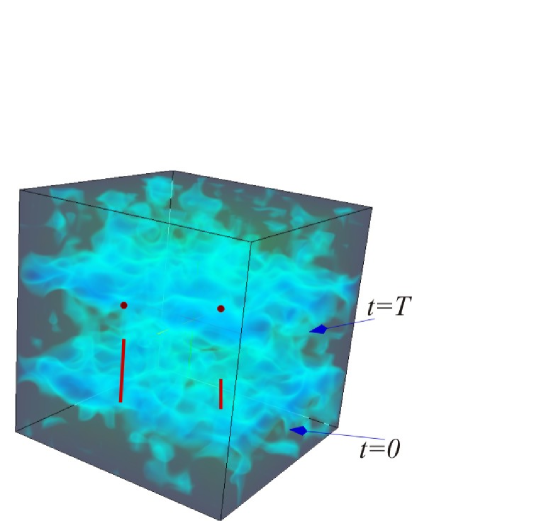
Figure 2: Illustration of the ice-limit: action density and orientation of the finite length Polyakov lines (vertical lines). The low action planes (at $t=0$ and $t=T$) are clearly visible.

The crucial idea to avoid any Gribov (or spin-glass) problem is to trivialise the orbit integration over $\Omega$ by factoring it out altogether. This can be done as follows. First note that in the matrix element $\rho_{\kappa}$ from (50) we may write

$$\Omega^{\dagger}(\boldsymbol{x},0)P[U](\boldsymbol{x},0,T)\Omega(\boldsymbol{x},T)=P[U^{\Omega}](\boldsymbol{x},0,T).$$

Hence, using the gauge invariance of action and Haar measure, we obtain for $N\rho_{\kappa}$

$$\int{\cal D}U_{\mu}\;{\cal D}\Omega\;\Omega^{\dagger}(\boldsymbol{x},0)P[U](\boldsymbol{x},0,T)\Omega(\boldsymbol{x},T)\,\Omega^{\dagger}(\boldsymbol{y},T)P^{\dagger}[U](\boldsymbol{y},0,T)\Omega(\boldsymbol{y},0)\;\mathrm{e}^{S_{\mathrm{YM}}[U]+S_{\mathrm{F}}[U^{\Omega}]}$$

$$= \int{\cal D}U_{\mu}\;{\cal D}\Omega\;P[U^{\Omega}](\boldsymbol{x},0,T)P^{\dagger}[U^{\Omega}](\boldsymbol{y},0,T)\;\mathrm{e}^{S_{\mathrm{YM}}[U]+S_{\mathrm{F}}[U^{\Omega}]}$$

$$= \int{\cal D}U^{\Omega}_{\mu}\;{\cal D}\Omega\;P[U^{\Omega}](\boldsymbol{x},0,T)P^{\dagger}[U^{\Omega}](\boldsymbol{y},0,T)\;\mathrm{e}^{S_{\mathrm{YM}}[U^{\Omega}]+S_{\mathrm{F}}[U^{\Omega}]}$$

$$= \Bigl{(}\int{\cal D}\Omega\Bigr{)}\,\int{\cal D}U_{\mu}\;P[U](\boldsymbol{x},0,T)P^{\dagger}[U](\boldsymbol{y},0,T)\;\mathrm{e}^{S_{\mathrm{YM}}[U]+S_{\mathrm{F}}[U]},$$

and, indeed, the gauge group integration factors out as a trivial volume factor, $\int{\cal D}\Omega=1$. Thus, our final answer for $\rho_{\kappa}$ becomes

$$\rho_{\kappa}(r,T) = N^{-1}\,\int{\cal D}U_{\mu}\;P[U](\boldsymbol{x},0,T)P^{\dagger}[U](\boldsymbol{y},0,T)\;\mathrm{e}^{S_{\mathrm{YM}}[U]+S_{\mathrm{F}}[U]}$$ (58)

$$N = \int{\cal D}U_{\mu}\;\mathrm{e}^{S_{\mathrm{YM}}[U]}.$$ (59)

It remains to discuss the strong gauge fixing limit. In contrast to (57) we now need to find the maximum of the gauge fixing action with respect to the links, $U_{\mu}$,

$$S_{\mathrm{F}}[U]\stackrel{{\scriptstyle U_{\mu}}}{{\longrightarrow}}\hbox{max}.$$ (60)

Crucially, this does not constitute a spin-glass problem as the global maximum of (60) is easily obtained:

$$U_{l}(\boldsymbol{x},t=0)=1,\hbox to28.45274pt{\hfill}U_{l}(\boldsymbol{x},t=T)=1,\hbox to28.45274pt{\hfill}l=1\ldots 3.$$ (61)

Hence, for infinitely large $\kappa$, the spatial links of the time-slices $t=0$ and $t=T$ are both frozen to the perturbative vacuum. We therefore call the limit $\kappa\to\infty$ the “ice-limit” of the integral dressing approach. The (finite length) Polyakov lines start and end on the frozen time slices. Figure 2 shows the action density in the cube consisting of the time axis and two spatial directions.

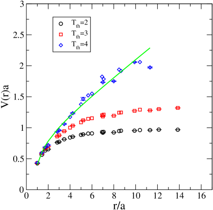
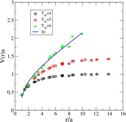
Figure 3: The static quark–antiquark potential from simulations with $\kappa=2.0$ (left) and in the ice-limit $\kappa=\infty$ (right).

We now present our numerical results. For finite values of $\kappa$ (with $\kappa$ not too large to avoid ergodicity problems in the spin-glass limit), we generated configurations $(U_{\mu},\Omega)$ corresponding to the partition function

$$\int{\cal D}U_{\mu}\;\mathrm{e}^{S_{\mathrm{YM}}[U]+S_{\mathrm{F}}[U]} = \int{\cal D}U_{\mu}\;{\cal D}\Omega\;\mathrm{e}^{S_{\mathrm{YM}}[U]+S_{\mathrm{F}}[U^{\Omega}]}\,,$$ (62)

$$S_{\mathrm{YM}}[U] = \beta\sum_{x,\mu>\nu}\frac{1}{2}\hbox{tr}\,P_{\mu\nu}[U](x)\,,$$ (63)

recalling $\int{\cal D}\Omega=1$. In order to ensure that the excited states are sufficiently suppressed, the Euclidean time $T$ must be chosen large enough. Here, we have considered all values $T\geq T_{\mathrm{th}}$ for the straight-line fit of

$$-\ln\rho(r,t)_{\kappa}=V(r)\,T\,-\,\ln|\langle 2|Q\bar{Q}\rangle|_{\kappa}^{2}$$ (64)

where the asymptotic form (48) of $\rho_{\kappa}(r,t)$ was used. Our final result for $V(r)a$ using a $16^{4}$ lattice, $\beta=2.3$ and $10000$ independent configurations is shown in Figure 3 (left panel). The line is a fit of the $T_{\mathrm{th}}=4$ data to

$$V(r)a=\sigma a^{2}\,\frac{r}{a}-\alpha/(r/a)+V_{0},\hbox to28.45274pt{\hfill}\sigma a^{2}(\beta=2.3)=0.14\;,$$ (65)

where the known value for the string tension in lattice units was used. We find that $T_{\mathrm{th}}=4$ is sufficient to decouple the excited states. A good agreement with the potential obtained with standard overlap enhancing techniques is observed.

We finally study the ice-limit $\kappa\to\infty$. In this case, configurations were generated using the standard partition function except that the spatial links in time slices $t=0$ and $t=T$ were fixed to unity. Using $\beta=2.3$ and a $16^{4}$ lattice, the static potential was extracted from $10,000$ independent configurations in the ice-limit. The result is shown in Figure 3 (right panel). We observe that rather large values for $T_{\mathrm{th}}$ are required to decouple the excited states in this case. One needs $T_{\mathrm{th}}=6$ to achieve good results for $V(r)$. Note, however, that no smearing was involved and gauge fixing ambiguities (‘Gribov noise’ [56]) are absent.

5 Conclusions

Non-perturbative gauge fixing is a key ingredient of many approaches to Yang-Mills theory. In order to have full analytic or numerical control all such approaches must confront and understand the Gribov problem as this unavoidably arises in any direct imposition of a gauge fixing condition. In this paper we have seen how to by-pass this problem both in the definition of an unambiguous partition function and in the construction of suitable mesonic states. To this end we have designed a novel and unified framework that combines the properly gauge fixed path integral introduced in [25, 26] and a generalised dressing approach based on group integration to construct gauge invariant states. The feasibility of this framework has been explicitly demonstrated for various examples ranging from the Christ-Lee model, U(1) gauge theory to SU(2) Yang-Mills theory.

From our new vantage point, the emergence of the Gribov problem could be traced back technically to a problem associated with the order of two integrations extending over the gauge orbits and field configurations, respectively. If the gauge group integration is performed before the average over the gluon fields, the Gribov problem arises as the problem to find the ground state of a spin-glass. However, since gauge invariance is manifest in our approach, the Gribov problem can be avoided by interchanging the integrations over gauge group and gluon fields. In this case, the (‘ice’) limit of strong gauge fixing can be performed analytically, and the external matter fields become properly dressed by gauge transformations unambiguously connected to the FMR of Coulomb gauge. The numerical feasibility of the method was finally demonstrated by a lattice calculation of the static quark antiquark potential from trial states in the ice limit, living on (initial and final) time slices frozen to the perturbative vacuum.

Acknowledgments: The authors thank Andreas Wipf for helpful discussions. The numerical calculations in this paper were carried out on the HPC and PlymGrid facilities at the University of Plymouth.

Appendix A Faddeev-Popov method and Gribov problem

The standard approach to (nonabelian) gauge fixing is the Faddeev-Popov method. Let us briefly recall it in the slightly generalised framework of [4, 5, 6]. In this modified approach one generalises the usual representation of unity (3) to the topological invariant

$$N[A] = \int{\cal D}\theta^{a}\;\hbox{Det}M[A]\;\delta\Bigl{(}\frac{\delta S_{\mathrm{fix}}[A^{\Omega}]}{\delta\theta^{a}(x)}\Bigr{)}$$ (66)

$$M[A]_{ab}(x,y) = \frac{\delta^{2}S_{\mathrm{fix}}[A^{\Omega}]}{\delta\theta^{a}(x)\delta\theta^{b}(y)}.$$ (67)

Under the idealising assumption that there is a unique solution to the gauge fixing condition (featuring in the $\delta$-function in (66)) the standard identity (3) is recovered,

$$N[A]=1\;,$$ (68)

with a gauge invariant Faddeev-Popov determinant, $\hbox{Det}M[A]=\hbox{Det}M[A^{g}]$. This may in turn be used to remove the gauge group volume from the partition function,

$$Z = \int{\cal D}A_{\mu}\;\mathrm{e}^{S[A]}=\int{\cal D}A_{\mu}\;{\cal D}\theta^{b}\;\hbox{Det}M[A]\;\delta\Bigl{(}\frac{\delta S_{\mathrm{fix}}[A^{\Omega}]}{\delta\theta^{a}(x)}\Bigr{)}\mathrm{e}^{S_{\mathrm{YM}}[A]}$$

$$= \int{\cal D}A^{\Omega}_{\mu}\;{\cal D}\theta^{b}\;\hbox{Det}M[A^{\Omega}]\;\delta\Bigl{(}\frac{\delta S_{\mathrm{fix}}[A^{\Omega}]}{\delta\theta^{a}(x)}\Bigr{)}\;\mathrm{e}^{S_{\mathrm{YM}}[A^{\Omega}]},$$

exploiting the invariance of the Haar measure, the action and the Faddeev-Popov determinant. Interchanging the order of integration and renaming $A^{\Omega}_{\mu}\rightarrow A_{\mu}$ finally yields

$$Z=\left(\int{\cal D}\theta^{b}\right)\;\int{\cal D}A_{\mu}\;\hbox{Det}M[A]\;\delta\Bigl{(}\frac{\delta S_{\mathrm{fix}}[A]}{\delta\theta^{a}(x)}\Bigr{)}\;\mathrm{e}^{S_{\mathrm{YM}}[A]}.$$ (69)

The latter equation is the desired result: the trivial factor from the gauge degeneracy has been factored out from the partition function, and the residual integration can be straightforwardly evaluated by means of perturbation theory.

The crucial observation, due to Gribov [2], is that the gauge fixing condition has many solutions. Hence, the group integration in (66) becomes a sum over all residual gauge transformations which cast a given background field $A_{\mu}$ into one of its Gribov copies. Due to the compactness of the group integration this implies that (68) is actually replaced by

$$N[A]=0\;,$$ (70)

so that also this generalised Faddeev-Popov approach remains ill-defined [5, 6] .

Appendix B Christ-Lee model revisited

In order to make contact with the Faddeev-Popov method we need to evaluate, from (12), the expression

$$S_{\mathrm{eff}}[\boldsymbol{x}]=S_{\mathrm{fix}}[\boldsymbol{x}]-\ln\int d\phi\;\mathrm{e}^{S_{\mathrm{fix}}[\boldsymbol{x}^{\phi}]}$$

for large values of $\kappa$, and for an arbitrary $S_{\text{fix}}$. To this end, let $\phi_{0}$ denote the gauge transformation which transports the vector $\boldsymbol{x}$ along its orbit to the global maximum of the gauge fixing action. For large $\kappa$ we may use a semi-classical approximation to evaluate $S_{\text{eff}}$, via:

$$\ln\int d\phi\;\mathrm{e}^{S_{\mathrm{fix}}[\boldsymbol{x}^{\phi}]} = S_{\mathrm{fix}}[\boldsymbol{x}^{\phi_{0}}]-\frac{1}{2}\ln M[\boldsymbol{x}]+\ln\sqrt{2\pi},$$ (71)

$$M[\boldsymbol{x}] = -\frac{\partial^{2}S_{\mathrm{fix}}[\boldsymbol{x}^{\phi}]}{\partial\phi^{2}}\Bigl{|}_{\phi=\phi_{0}},$$ (72)

where $M$ is the gauge invariant “Faddeev-Popov matrix”. It follows that (12) becomes

$$Z=\left(2\pi\right)\,\int d^{2}x\;\mathrm{e}^{S_{{}_{\mathrm{CL}}}(\boldsymbol{x})}\,\mathrm{e}^{S_{\mathrm{fix}}[\boldsymbol{x}]-S_{\mathrm{fix}}[\boldsymbol{x}^{\phi_{0}}]}\,\mathrm{e}^{\frac{1}{2}\ln M[x]-\ln\sqrt{2\pi}}\;.$$ (73)

For $S_{\mathrm{fix}}[\boldsymbol{x}^{\phi}]$ as in (9) with $\boldsymbol{v}=(1,0)$ and for a given vector $\boldsymbol{x}=(x,y)$, $\phi_{0}[\boldsymbol{x}]$ is defined by

$$x\,\cos\phi_{0}\,-\,y\,\sin\phi_{0}\stackrel{{\scriptstyle\phi_{0}}}{{\to}}\hbox{max}.$$

This implies

$$x\,\cos\phi_{0}[\boldsymbol{x}]\,-\,y\,\sin\phi_{0}[\boldsymbol{x}]=r,\hbox to28.45274pt{\hfill}S_{\mathrm{fix}}[\boldsymbol{x}^{\phi_{0}}]=-\frac{\kappa}{2}\big{(}r-1)^{2}.$$

and indeed the Faddeev-Popov matrix is gauge invariant, $M[\boldsymbol{x}]=\kappa r$.

Returning to a general $S_{\text{fix}}$, consider the weight factor $P(\boldsymbol{x})=\exp\{S_{\mathrm{fix}}[\boldsymbol{x}]-S_{\mathrm{fix}}[\boldsymbol{x}^{\phi_{0}}]\}$. This will restrict the field (here, $\boldsymbol{x}$) integration to the FMR for large values of $\kappa$. To show this, it is convenient to decompose the vector $\boldsymbol{x}$ into a part $\boldsymbol{x}_{{}_{\mathrm{FMR}}}\in\hbox{FMR}$ and a fluctuation along the gauge orbit,

$$\boldsymbol{x}=\boldsymbol{x}_{{}_{\mathrm{FMR}}}^{\varphi}.$$

In contrast to the Faddeev-Popov approach, this must not be done for the 2-dimensional space as a whole but only locally for $\boldsymbol{x}$ close to the FMR. Since

$$\frac{\partial S_{\mathrm{fix}}[\boldsymbol{x}^{\varphi}]}{\partial\varphi}\Bigl{|}_{\boldsymbol{x}\in\boldsymbol{x}_{{}_{\mathrm{FMR}}}}=0,$$

we are led to

$$\mathrm{e}^{S_{\mathrm{fix}}[\boldsymbol{x}]-S_{\mathrm{fix}}[\boldsymbol{x}^{\varphi_{0}}]}=h(\boldsymbol{x}_{{}_{\mathrm{FMR}}})\,\delta\left(\frac{\partial S_{\mathrm{fix}}[\boldsymbol{x}^{\varphi}]}{\partial\varphi}\Bigl{|}_{\boldsymbol{x}\in\boldsymbol{x}_{{}_{\mathrm{FMR}}}}\right).$$ (74)

The weight function $h(\boldsymbol{x}_{{}_{\mathrm{FMR}}})$ can be calculated by integrating $\varphi$ over a small interval around zero. We will assume that the map $\boldsymbol{x}\leftrightarrow(\boldsymbol{x}_{{}_{\mathrm{FMR}}},\varphi)$ is invertible for $\boldsymbol{x}$ in a region around the FMR. We stress, however, that this depends on the gauge choice and might not be the case for more general settings thus hinting at a shortcoming of the Faddeev-Popov approach. Under the above assumption, we use

$$\int d\varphi\;M(\boldsymbol{x}_{{}_{\mathrm{FMR}}})\delta\left(\frac{\partial S_{\mathrm{fix}}[\boldsymbol{x}^{\varphi}]}{\partial\varphi}\Bigl{|}_{\boldsymbol{x}\in\boldsymbol{x}_{{}_{\mathrm{FMR}}}}\right)=1\;$$

and find

$$h(\boldsymbol{x}_{{}_{\mathrm{FMR}}})=\int d\varphi\;M(\boldsymbol{x}_{{}_{\mathrm{FMR}}})\;\mathrm{e}^{S_{\mathrm{fix}}[\boldsymbol{x}]-S_{\mathrm{fix}}[\boldsymbol{x}^{\varphi_{0}}]}\stackrel{{\scriptstyle\cdot}}{{=}}M(\boldsymbol{x}_{{}_{\mathrm{FMR}}})\int d\varphi\;\mathrm{e}^{-\frac{1}{2}M(\boldsymbol{x}_{{}_{\mathrm{FMR}}})\,\varphi^{2}}=\sqrt{2\pi M(\boldsymbol{x}_{{}_{\mathrm{FMR}}})}.$$ (75)

Inserting (75) and (74) in (73), we finally obtain the desired result,

$$Z=\left(2\pi\right)\,\int d^{2}x\;\mathrm{e}^{S_{{}_{\text{CL}}}(\boldsymbol{x})}\,M(\boldsymbol{x}_{{}_{\mathrm{FMR}}})\,\delta\left(\frac{\partial S_{\mathrm{fix}}[\boldsymbol{x}^{\varphi}]}{\partial\varphi}\Bigl{|}_{\boldsymbol{x}\in\boldsymbol{x}_{{}_{\mathrm{FMR}}}}\right),$$ (76)

which is the starting point of the Faddeev-Popov method.

References

- [1] L. D. Faddeev and V. N. Popov, Phys. Lett. B 25, 29 (1967).
- [2] V. N. Gribov, Nucl. Phys. B 139, 1 (1978).
- [3] I. M. Singer, Commun. Math. Phys. 60, 7 (1978).
- [4] H. Neuberger, Phys. Lett. B 183, 337 (1987).
- [5] L. Baulieu, A. Rozenberg and M. Schaden, Phys. Rev. D 54, 7825 (1996) [arXiv:hep-th/9607147].
- [6] L. Baulieu and M. Schaden, Int. J. Mod. Phys. A 13, 985 (1998) [arXiv:hep-th/9601039].
- [7] D. Zwanziger, Nucl. Phys. B 192, 259 (1981).
- [8] L. Baulieu and D. Zwanziger, Nucl. Phys. B 193, 163 (1981).
- [9] M. Horibe, A. Hosoya and J. Sakamoto, Prog. Theor. Phys. 70, 1636 (1983).
- [10] D. Zwanziger, Phys. Rev. D 69, 016002 (2004) [arXiv:hep-ph/0303028].
- [11] L. von Smekal, A. Hauck and R. Alkofer, Annals Phys. 267, 1 (1998) [Erratum-ibid. 269, 182 (1998)] [arXiv:hep-ph/9707327].
- [12] L. von Smekal, R. Alkofer and A. Hauck, Phys. Rev. Lett. 79, 3591 (1997) [arXiv:hep-ph/9705242].
- [13] R. Alkofer and L. von Smekal, Phys. Rept. 353, 281 (2001) [arXiv:hep-ph/0007355].
- [14] H. Suman and K. Schilling, Phys. Lett. B 373, 314 (1996) [arXiv:hep-lat/9512003].
- [15] A. Cucchieri, Nucl. Phys. B 508, 353 (1997) [arXiv:hep-lat/9705005].
- [16] J. C. R. Bloch, A. Cucchieri, K. Langfeld and T. Mendes, Nucl. Phys. B 687, 76 (2004) [arXiv:hep-lat/0312036].
- [17] D. B. Leinweber, J. I. Skullerud, A. G. Williams and C. Parrinello [UKQCD Collaboration], Phys. Rev. D 60, 094507 (1999) [Erratum-ibid. D 61, 079901 (2000)] [arXiv:hep-lat/9811027].
- [18] F. D. R. Bonnet, P. O. Bowman, D. B. Leinweber, A. G. Williams and J. M. Zanotti, Phys. Rev. D 64, 034501 (2001) [arXiv:hep-lat/0101013].
- [19] K. Langfeld, H. Reinhardt and J. Gattnar, Nucl. Phys. B 621, 131 (2002) [arXiv:hep-ph/0107141].
- [20] C. S. Fischer, R. Alkofer and H. Reinhardt, Phys. Rev. D 65, 094008 (2002) [arXiv:hep-ph/0202195].
- [21] I. L. Bogolubsky, E. M. Ilgenfritz, M. Muller-Preussker and A. Sternbeck, PoS LATTICE, 290 (2007) [arXiv:0710.1968 [hep-lat]].
- [22] A. Cucchieri and T. Mendes, arXiv:0804.2371 [hep-lat].
- [23] D. Dudal, S. P. Sorella, N. Vandersickel and H. Verschelde, Phys. Rev. D 77, 071501 (2008) [arXiv:0711.4496 [hep-th]].
- [24] D. Dudal, J. Gracey, S. P. Sorella, N. Vandersickel and H. Verschelde, arXiv:0806.4348 [hep-th].
- [25] C. Parrinello and G. Jona-Lasinio, Phys. Lett. B 251, 175 (1990).
- [26] D. Zwanziger, Nucl. Phys. B 345, 461 (1990).
- [27] S. Fachin and C. Parrinello, Phys. Rev. D 44, 2558 (1991).
- [28] C. Parrinello and S. Fachin, Nucl. Phys. Proc. Suppl. 26, 429 (1992).
- [29] D. S. Henty, O. Oliveira, C. Parrinello and S. Ryan [UKQCD Collaboration], Phys. Rev. D 54, 6923 (1996) [arXiv:hep-lat/9607014].
- [30] V. K. Mitrjushkin and A. I. Veselov, JETP Lett. 74, 532 (2001) [Pisma Zh. Eksp. Teor. Fiz. 74, 605 (2001)] [arXiv:hep-lat/0110200].
- [31] C. Aubin and M. C. Ogilvie, Phys. Rev. D 70, 074514 (2004) [arXiv:hep-lat/0406014].
- [32] A. M. Polyakov, Phys. Lett. B 72, 477 (1978).
- [33] L. Susskind, Phys. Rev. D 20, 2610 (1979).
- [34] D. J. Gross, R. D. Pisarski and L. G. Yaffe, Rev. Mod. Phys. 53, 43 (1981).
- [35] G. Marchesini and E. Onofri, Nuovo Cim. A 65, 298 (1981).
- [36] K. Zarembo, Mod. Phys. Lett. A 13, 2317 (1998) [arXiv:hep-th/9806150].
- [37] K. Zarembo, arXiv:hep-th/9808189.
- [38] J. R. Klauder, Annals Phys. 254, 419 (1997) [arXiv:quant-ph/9604033].
- [39] J. R. Klauder, Nucl. Phys. B 547, 397 (1999) [arXiv:hep-th/9901010].
- [40] V. M. Villanueva, J. Govaerts and J. L. Lucio-Martinez, J. Phys. A 33, 4183 (2000) [arXiv:hep-th/9909033].
- [41] J. D. Jackson and L. B. Okun, Rev. Mod. Phys. 73, 663 (2001) [arXiv:hep-ph/0012061].
- [42] G. ’t Hooft, Nucl. Phys. B 190, 455 (1981).
- [43] M.A. Semenov-Tyan-Shanskii and V.A. Franke, Zapiski Nauchnykh Seminarov Leningradskogo Otdeleniya Matematicheskogo Instituta im. V.A. Steklov AN SSSR, 120 159 (1982); [Translation: (Plenum, New York, 1986), p. 1999.
- [44] D. Zwanziger, Nucl. Phys. B 209, 336 (1982).
- [45] P. van Baal, Nucl. Phys. B 369, 259 (1992).
- [46] J. Fuchs, M. G. Schmidt and C. Schweigert, Nucl. Phys. B 426, 107 (1994) [arXiv:hep-th/9404059].
- [47] P. van Baal, arXiv:hep-ph/0008206.
- [48] M. E. Peskin and D. V. Schroeder, “An Introduction To Quantum Field Theory”, Addison-Wesley (1995).
- [49] N. H. Christ and T. D. Lee, Phys. Rev. D 22, 939 (1980) [Phys. Scripta 23, 970 (1981)].
- [50] D. Zwanziger, Nucl. Phys. B 323, 513 (1989).
- [51] D. Zwanziger, Nucl. Phys. B 412, 657 (1994).
- [52] M. Lavelle and D. McMullan, Phys. Rept. 279, 1 (1997) [arXiv:hep-ph/9509344].
- [53] E. Bagan, M. Lavelle and D. McMullan, Annals Phys. 282 (2000) 471 [arXiv:hep-ph/9909257].
- [54] E. Bagan, M. Lavelle and D. McMullan, Annals Phys. 282 (2000) 503 [arXiv:hep-ph/9909262].
- [55] A. Ilderton, M. Lavelle and D. McMullan, JHEP 0703 (2007) 044 [arXiv:hep-th/0701168].
- [56] T. Heinzl, K. Langfeld, M. Lavelle and D. McMullan, Phys. Rev. D 76, 114510 (2007) [arXiv:0705.2718 [hep-lat]].
- [57] I. Montvay and G. Münster, “Quantum fields on a lattice”, Cambridge University Press (1994).
- [58] T. Heinzl, A. Ilderton, K. Langfeld, M. Lavelle, W. Lutz and D. McMullan, Phys. Rev. D 77, 054501 (2008) [arXiv:0709.3486 [hep-lat]].
- [59] T. Heinzl, A. Ilderton, K. Langfeld, M. Lavelle, W. Lutz and D. McMullan, arXiv:0806.1187 [hep-lat].