Higher Powers in Gravitation

Abstract

We consider the Friedmann-Robertson-Walker cosmologies of theories of gravity that generalise the Einstein-Hilbert action by replacing the Ricci scalar, $R$, with some function, $f(R)$. The general asymptotic behaviour of these cosmologies is found, at both early and late times, and the effects of adding higher and lower powers of $R$ to the Einstein-Hilbert action is investigated. The assumption that the highest powers of $R$ should dominate the Universe’s early history, and that the lowest powers should dominate its future is found to be inaccurate. The behaviour of the general solution is complicated, and while it can be the case that single powers of $R$ dominate the dynamics at late times, it can be either the higher or lower powers that do so. It is also shown that it is often the lowest powers of $R$ that dominate at early times, when approach to a bounce or a Tolman solution are generic possibilities. Various examples are considered, and both vacuum and perfect fluid solutions investigated.

1 Introduction

We study here the dynamics of Friedmann-Robertson-Walker (FRW) universes in $f(R)$ theories of gravity. These theories are derived from generalisations of the usual Einstein-Hilbert Lagrangian of General Relativity (GR), such that

$$\mathcal{L}=f(R),$$ (1)

and have been considered extensively in the literature (see e.g. [1, 2, 3, 4]). Specification of the function $f(R)$ defines the theory, and GR can be seen to be the special case $f=R$. Such theories have drawn considerable interest as they found success in early attempts to create a perturbatively re-normalisable quantum field theory of gravity [5], as well as turning up more recently in the effective actions of string theory [6, 7]. In cosmology these theories have been used extensively in attempts to explain the late-time accelerating expansion of the Universe [8, 9], cosmological inflation [10, 11, 12] and the nature of the initial singularity [13, 14, 15]. For a recent review see [16].

In considering generalised $f(R)$ theories of gravity it is often implicitly assumed that at late times in the evolution of the Universe it should be the lowest powers of $R$ that dominate the gravitational Lagrangian. That is, at late times we should have $R\rightarrow 0$, and the Universe should behave as if it were governed by a gravitational Lagrangian of the form

$$\mathcal{L}_{0}=\lim_{R\to 0}f(R),$$ (2)

which is often presumed to correspond to the Einstein-Hilbert Lagrangian, although other limits have been considered in attempts to address the apparent late-time acceleration of the Universe [8, 9]. Conversely, the introduction of higher powers of $R$ into the gravitational Lagrangian has often been assumed to mean that at early times the Universe should behave as if governed by the vacuum dynamics of a Lagrangian

$$\mathcal{L}_{\infty}=\lim_{R\to\infty}f(R).$$ (3)

The picture is then one of a universe that starts off at high $R$, dominated by a Lagrangian of the form (3), and that subsequently expands until $R$ becomes small and the gravitational dynamics are dominated by a Lagrangian of the form (2). It is the purpose of this paper to determine the veracity of such assumptions. This is achieved by studying the dynamical evolution of FRW universes, governed by theories with general $f(R)$. The asymptotic behaviour of the general solution to the Friedmann equations is then investigated, and used to evaluate the extent to which the afore mentioned behaviour may be considered generic.

The general solutions of FRW cosmologies governed by $f(R)$ theories of gravity have been studied previously by a number of authors, in a number of different contexts. Much of this work has made use of the dynamical systems approach, which has been used to study specific classes of $f(R)$ in isotropic cosmologies in [17, 18, 19], and anisotropic cosmologies in [20, 21, 22]. Exact analytic expressions have been found for the general FRW solutions of some $f(R)$ theories in [23], and the dynamical systems approach applied to general $f(R)$ has been considered in [24]. For studies of spherically symmetric and weak field solutions see [16, 17, 26, 27], and references therein. The approach used here is a generalisation of the analysis performed in [17], where theories of the form $f\propto R^{n}$ were considered.

We find here that the late-time attractors of FRW cosmologies for general $f(R)$ have various different forms, and that the asymptote toward which the general solution is attracted depends upon the initial conditions. Some of these solutions correspond to the lowest powers of $f(R)$ dominating at late-times, and others to the highest powers. Expanding universes with powers of $R$ lower than $R^{2}$ dominating their dynamics generically appear to exhibit the former behaviour, while universes with powers of $R$ greater than $R^{2}$ dominating appear to generically exhibit the latter. Expanding universes with higher powers of $R$ dominating their early evolution therefore appear unlikely to evolve to a state where the Einstein-Hilbert term dominates.

We also find that there usually exist multiple early-time attractors for the general solution. These can take on different forms, but generically it appears that they either evolve as $a\sim t^{\frac{1}{2}}$, toward a big bang singularity in the past, or that they approach a point of inflexion, where the scale factor is constant. This is in good agreement with the analytic general solutions for $f\propto R^{n}$ found in [23]. These results do not mean that a period of inflation cannot occur (as indeed it appears to if $f\sim R^{2}$), but it does mean that the general solution does not generally start off inflating (even if $f\sim R^{2}$). It also means that the picture of the highest powers of $R$ dominating the earliest stages of the Universe’s evolution may not be an accurate one.

We begin in section 2 by giving the FRW field equations for $f(R)$ theories, together with some simple power-law particular solutions that will later appear as asymptotes of the general solution. In section 3 we use a dynamical systems approach to determine the form of the general solution for vacuum cosmologies. The phase space of the general solution is two dimensional, and the location and stability of critical points in this space is determined. In section 4 we perform a similar analysis for the case of perfect fluid cosmologies. The phase space of the general solution is now three dimensional, and the location and stability of critical points is again determined. In section 5 we consider the effect of adding higher and lower powers of $R$ to the Einstein-Hilbert action. Section 6 provides a discussion of the results, and the appendix gives some special cases that are of particular interest.

2 f(R) Cosmology

2.1 Field Equations

Replacing the Ricci scalar, $R$, in the Einstein-Hilbert action by a more general function, $f(R)$, gives the Lagrangian density

$$\mathcal{L}=f(R)+\mathcal{L}_{m},$$ (4)

where $\mathcal{L}_{m}$ is the Lagrangian density of matter fields. Variation of the corresponding action, with respect to the metric, gives the field equations

$$f_{R}R_{ab}-\frac{1}{2}fg_{ab}+{f_{R;}}^{cd}(g_{ab}g_{cd}-g_{ac}g_{bd})=8\pi T_{ab},$$ (5)

where $f_{R}\equiv\delta f/\delta R$, and $T_{ab}$ is the energy-momentum tensor of matter fields, defined in the usual way. The Lagrangian formulation of the theory guarantees the conservation equations ${T^{ab}}_{;b}=0$.

Substituting the FRW metric into the field equations, (5), gives the analogue of the Friedmann equations

$$-3\frac{\ddot{a}}{a}f_{R}+\frac{1}{2}f+3\frac{\dot{a}}{a}\dot{f}_{R} =8\pi\rho$$ (6)

$$-f_{R}R+2f+3\left(\ddot{f}_{R}+3\frac{\dot{a}}{a}\dot{f}_{R}\right) =8\pi(4-3\gamma)\rho,$$ (7)

where $a=a(t)$ is the scale factor, and here we have assumed the matter fields are well described by a perfect fluid, with barotropic equation of state $p=(\gamma-1)\rho$. The conservation equations are then, as usual,

$$\dot{\rho}+3\gamma\frac{\dot{a}}{a}\rho=0,$$ (8)

and the Ricci scalar is

$$R=\frac{1}{6}\left(\frac{\ddot{a}}{a}+\frac{\dot{a}^{2}}{a^{2}}+\frac{k}{a^{2}}\right),$$ (9)

where $k$ is the constant curvature of homogeneous spatial 3-surfaces. Henceforth, unless explicitly stated otherwise, we will be considering only the spatially flat class of models, where $k=0$. Spatially curved models will be investigated elsewhere.

2.2 Particular Solutions

The field equations (6)-(9) have a number of particular solutions that are of interest. These solutions often act as attractors, toward which the general solutions can asymptote. Such behaviour will be shown in subsequent sections.

First let us consider the ‘vacuum dominated’ solution

$$\hskip 150.0pta\sim(t-t_{0})^{\frac{B_{0}(1+B_{0})}{1-3B_{0}+2B_{0}^{2}}}$$ [vacuum dominated solution] (10)

where $t_{0}$ is a constant, and $B_{0}$ is defined as

$$B_{0}\equiv 1-\frac{f}{Rf_{R}}\rightarrow\text{constant}.$$ (11)

That $B_{0}\rightarrow$constant is a requirement on the theory in order for the solution to exist. Equation (10) represents a cosmology in which the evolution of the scale factor is dominated by the dynamics of the Ricci curvature itself. It is this type of evolution that is often invoked to account for the late-time acceleration of the Universe, or its inflation at early times. In the limit that GR is approached, and $B_{0}\rightarrow 0$, this solution reduces to Minkowski space.

Another solution of interest is the ‘matter dominated’ solution

$$\hskip 150.0pta\sim(t-t_{0})^{\frac{2}{3\gamma(1-B_{0})}}.$$ [matter dominated solution] (12)

Again, this solution exists if $B_{0}\rightarrow$constant (not necessarily the same constant as in (10)). This solution, if it exists, is dependent on the matter content of the space-time, as can be seen from the explicit dependence on $\gamma$. As $B_{0}\rightarrow 0$, and GR is approached, this solution reduces to the usual spatially flat, perfect fluid dominated Friedmann solution.

The last particular solution of interest is the Tolman solution

$$\hskip 150.0pta\sim(t-t_{0})^{\frac{1}{2}}.$$ [Tolman solution] (13)

This solution is independent of both the matter content of the Universe, and of the form of $f(R)$. We call it the Tolman solution as it is identical to the radiation dominated Friedmann solution of GR. However, this solution does not necessarily require the presence of either radiation ($\gamma=4/3$), or of an Einstein-Hilbert term in the action.

We will now proceed to investigate the form of the general solutions to equations (6)-(9), first for the vacuum case ($\rho=0$), and then for the perfect fluid case ($\rho\neq 0$). The particular solutions above will often appear as the asymptotic form of the general solution, as $t\rightarrow\pm\infty$ or $t_{0}=$constant.

3 Vacuum Cosmologies

3.1 The Dynamical System

In the case of vacuum cosmologies we have $\rho=0$. The field equations (6)-(9) can now be transformed into a system of first-order differential equations, by defining the time coordinate $d\tau\equiv\sqrt{|R|}dt$, and the new variables $x\equiv a^{\prime}/a$, $y\equiv f_{R}^{\prime}/f_{R}$ and $z\equiv\ln|R|$. The equations (6)-(9) then become

$$x^{\prime} =\frac{Q}{6}-2x^{2}-Axy$$ (14)

$$y^{\prime} =4x^{2}+xy-y^{2}-\frac{Q}{3}-Ay^{2}$$ (15)

$$z^{\prime} =2Ay,$$ (16)

with the constraint

$$x^{2}+xy-\frac{1}{6}BQ=0,$$ (17)

where primes denote differentiation with respect to $\tau$, and $Q\equiv$sign$(R)$. These definitions ensure $\tau$ is always real, and monotonically increasing in $t$. The two new functionals $A=A(z)$ and $B=B(z)$ are defined by $A\equiv f_{R}/2Rf_{RR}$ and $B\equiv 1-f/Rf_{R}$. Specifying $f(R)$ gives $A(z)$ and $B(z)$, and the system of equations (14)-(17) is closed. However, even before specifying $f(R)$ it is possible to determine some generic features of the system above, and hence of vacuum $f(R)$ FRW cosmologies in general. The form of equations (14)-(17) allow us to treat the problem as a dynamical system, in which the general solutions for $f(R)$ vacuum FRW cosmologies are given as trajectories in the phase space ($x$,$y$,$z$). Such an analysis will allow insight into the behaviour of these models.

First we note that the surface $R=0$ is an invariant sub-manifold of the ($x$,$y$,$z$) phase space. From (17) it can be seen that $R=0$ corresponds to $x^{2}+xy=0$. Equations (14)-(17) then give

$$(x^{2}+xy)^{\prime}=-y(x^{2}+xy)(1+2A-1/B),$$ (18)

so there are no trajectories in ($x$, $y$,$z$) that allow $R$ to change sign along them. This justifies our choice of $z$.

It is now convenient to perform a transformation from the infinite plane spanned by ($x$, $y$), to a finite closed space. This can be achieved by the re-definitions $x\equiv r\cos\theta$ and $y\equiv r\sin\theta$, which give

$$\theta^{\prime} =-Q\left[2(1-2B)\cos\theta+(1+B)\sin\theta\right]\sqrt{\frac{1+\cos(2\theta)+\sin(2\theta)}{12BQ}}$$ (19)

$$z^{\prime} =2AP\sqrt{\frac{BQ}{6\cot\theta(1+\cot\theta)}},$$ (20)

where the constraint (17) has been used, $P$ is the sign of $y$, and $\theta$ runs from $0$ to $2\pi$. It can now be seen that, independent of the value of $B$, there exist stationary points in ($x$,$y$) at

$$\theta_{1}=-\pi/2,\qquad\theta_{2}=\pi/2,\qquad\theta_{3}=-\pi/4\qquad\text{and}\qquad\theta_{4}=3\pi/4.$$ (21)

In the limit $B\rightarrow B_{0}=$constant or $\pm\infty$, if this exists, there are two further stationary points in the ($x$,$y$) plane at

$$\tan\theta_{5,6}=\frac{2(2B_{0}-1)}{(B_{0}+1)}.$$ (22)

The value of $B_{0}$, and the existence of these last two points, depends on the form of $f(R)$, and can be straight-forwardly deduced once this function is specified. Various cases will be considered in later sections. First we will investigate the behaviour of the scale factor at the points $1-6$, identified above.

From the definitions of $x$ and $y$ we have, at stationary $\theta_{i}$, that

$$\frac{f_{R}^{\prime}}{f_{R}}=\tan\theta_{i}\frac{a^{\prime}}{a},$$ (23)

which can be integrated to obtain $f_{R}\propto a^{\tan\theta_{i}}$. Eliminating $f$ in equations (6) and (7), and substituting for $f_{R}$, then gives

$$\frac{\ddot{a}_{i}}{a_{i}}=\frac{(2+2\tan\theta_{i}-\tan^{2}\theta_{i})}{(2+\tan\theta_{i})}\frac{\dot{a}^{2}_{i}}{a^{2}_{i}},$$ (24)

which, for $\tan\theta_{i}\neq 0$ or $1$, integrates to

$$a_{i}=a_{0}|t-t_{0}|^{\frac{(2+\tan\theta_{i})}{\tan\theta_{i}(\tan\theta_{i}-1)}},$$ (25)

where $a_{0}$ and $t_{0}$ are constants. Substituting $\theta_{i}$ from points $1-6$ then gives the form of the scale factor as these points are approached. For the special cases $\tan\theta_{i}=0$ or $1$ we instead have

$$a_{i}=a_{0}e^{c(t-t_{0})},$$ (26)

where $c$ is a constant. For points $5$ and $6$ this corresponds to $B_{0}=1/2$ or $1$.

The stationary points $1$ and $2$ can now be seen to correspond to $a^{\prime}/a=0$, and points $3$ and $4$ to the Tolman solution, (13). For $B\neq 1/2$ or $1$ we find points $5$ and $6$ correspond to the vacuum dominated solution, (10). These results are summarised in Table 1, where symbols refer to those used in Figure 1.

Point	a(t)	Symbol
1, 2	$a^{\prime}/a=0$	Circle
3, 4	Tolman solution, (13)	Square
5, 6	Vacuum dominated solution, (10)	Triangle

Table 1: The evolution of the scale factor, $a(t)$, at the critical points $1$-$6$ in vacuum $f(R)$ cosmologies. The listed symbols correspond to those used in Figure 1.

3.2 Stability Properties

Having determined the location of the stationary points in the ($x$,$y$) plane, and the scale factors to which they correspond, we will now investigate their stability properties. This will allow us to determine which points are stable, and can act as asymptotic attractors of the general solution, and which are unstable, and can act as repellors (i.e. attractors in the asymptotic past, if time is run backwards).

The stability of points $1$ to $6$ can be determined as follows. Begin by perturbing $\theta$ as

$$\theta\rightarrow\theta_{i}+\delta\theta_{i},$$ (27)

where $\delta\theta_{i}$ is small. For points at finite $z=z_{i}$ also perturb $z$, $A$ and $B$ as

$$z \rightarrow z_{i}+\delta z_{i}$$ (28)

$$A \rightarrow A(z_{i})+\left(\frac{dA}{dz}\right)_{z=z_{i}}\delta z_{i}$$ (29)

$$B \rightarrow B(z_{i})+\left(\frac{dB}{dz}\right)_{z=z_{i}}\delta z_{i}.$$ (30)

For points at infinite $z$ we need only to perturb $\theta$, and to check the sign of $z^{\prime}$, in order to determine stability.

Points $1$ and $2$, to linear order in perturbations, then give

$$\delta\theta_{1,2}^{\prime} \rightarrow\mp\frac{(1+B_{1,2})}{2B_{1,2}}\sqrt{\frac{QB_{1,2}}{3(1+\cos(2\theta_{1,2})+\sin(2\theta_{1,2}))}}\delta\theta_{1,2}$$ (31)

$$\sim\text{sign}\left\{\mp\frac{(1+B_{1,2})}{B_{1,2}}\right\}\delta\theta_{1,2}$$ (32)

where the upper sign is for point $1$, and the lower sign for point $2$. This expression is independent of any $\delta z$, and so is valid for all points at finite or infinite $z$.

For points $3$ and $4$ we have

$$\delta\theta_{3,4}^{\prime} \rightarrow\pm\frac{(5B_{3,4}-1)}{4B_{3,4}}\sqrt{\frac{2QB_{3,4}}{3(1+\cos(2\theta_{3,4})+\sin(2\theta_{3,4}))}}\delta\theta_{3,4}$$ (33)

$$\sim\text{sign}\left\{\pm\frac{(5B_{3,4}-1)}{B_{3,4}}\right\}\delta\theta_{3,4},$$ (34)

where the upper sign is for point $3$, and the lower for point $4$. Again, this is independent of any $\delta z$. Points $1$ to $4$ are therefore stable attractors if $\delta\theta^{\prime}/\delta\theta<0$, and unstable repellors if $\delta\theta^{\prime}/\delta\theta>0$.

Now consider the stability of points $5$ and $6$. In this case a knowledge of the behaviour of $z$ is necessary to determine stability in the ($x$,$y$) plane. For $B_{0}\neq 1/2$ or $1$ the Ricci scalar corresponding to the vacuum solution (10) is given by

$$R_{5,6} =\frac{B_{0}(1+B_{0})(5B_{0}-1)}{6(1-3B_{0}+2B_{0}^{2})^{2}(t-t_{0})^{2}}$$ (35)

$$\propto\exp\left\{\mp 2\sqrt{\frac{6(1-3B_{0}+2B_{0}^{2})^{2}}{|B_{0}(1+B_{0})(5B_{0}-1)|}}(\tau-\tau_{0})\right\},$$ (36)

where the upper branch in the final line is for $t>t_{0}$, and the lower branch for $t<t_{0}$. As $\tau\rightarrow\pm\infty$, we then have that $R_{5,6}\rightarrow\pm\infty$ or $0$. These points therefore exist at finite $\theta$ and infinite $z$. As such we can check their stability by perturbing $\theta$, as before, and checking the sign of $z^{\prime}$ as $\tau\rightarrow\pm\infty$. From (36) it can be immediately seen that for $t>t_{0}$ we have $z^{\prime}<0$, so when $\delta\theta^{\prime}/\delta\theta<0$ this is a stable point in ($x$,$y$,$z$), and corresponds to $R\rightarrow 0$ as $\tau\rightarrow\infty$. Similarly, for $t>t_{0}$ it can be seen that when $\delta\theta^{\prime}/\delta\theta>0$ this is an unstable point, corresponding to $R\rightarrow\pm\infty$ as $\tau\rightarrow-\infty$. The condition for the existence of points $5$ and $6$, when $t>t_{0}$, can now be seen to be $B\rightarrow B_{0}$ as $z\rightarrow\mp\infty$, for stable or unstable points, respectively. Similar behaviour can be seen to be true when $t<t_{0}$, with the opposite limits taken for $z$ in each case. Substituting $\theta\rightarrow\theta_{5,6}+\delta\theta_{5,6}$ into (19) now gives

$$\delta\theta_{5,6}^{\prime} \rightarrow\mp\frac{(5B_{0}-1)}{B_{0}\sqrt{1+\frac{4(1-2B_{0})^{2}}{(1+B_{0})^{2}}}}\sqrt{\frac{QB_{0}}{3(1+\cos(2\theta_{0})+\sin(2\theta_{0}))}}\delta\theta_{5,6}$$ (37)

$$\sim\text{sign}\left\{\mp\frac{(5B_{0}-1)}{B_{0}}\right\}\delta\theta_{5,6}.$$ (38)

The upper sign here corresponds to $\theta_{5}\in(-\pi/2,\pi/2)$, and the lower sign to $\theta_{6}\in(\pi/2,3\pi/2)$. For the special cases $B_{0}=1/2$ or $1$ the asymptotic value of $z$ is a finite constant. In these cases the stability analysis must include a perturbation to $z$, and the corresponding perturbations this induces in $A(z)$ and $B(z)$. We perform this analysis in Appendix A. For these cases we find that it is possible for points $5$ or $6$ to initially act as attractors, while later acting as saddle points. We call this behaviour ‘semi-stable’, and describe it more fully in the appendix.

The stability properties of the critical points $1-6$ are summarised in Table 2. Here ‘A’ stands for (stable) Attractor, and ‘R’ for (unstable) Repellor.

Point	Stability
	$\mathbf{B<-1}$	$\mathbf{-1<B<0}$	$\mathbf{0<B<1/5}$	$\mathbf{1/5<B}$
1	A	R	A	A
2	R	A	R	R
3	R	R	A	R
4	A	A	R	A
5	A	A	R	A
6	R	R	A	R

Table 2: The stability properties of the critical points $1$-$6$ in vacuum $f(R)$ cosmologies. ‘A’ denotes a stable Attractor, and ‘R’ denotes an unstable Repellor.

3.3 The General Solution

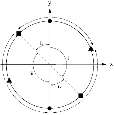
(a) The ($x$,$y$) plane when $B<-1$ or $B>1/5$. In this case the triangles, corresponding to the critical points (39), are located in the intervals ($-\pi/4$,$\pi/2$) and ($3\pi/4$,$-\pi/2$). Arrows denote the direction of trajectories around the circle.

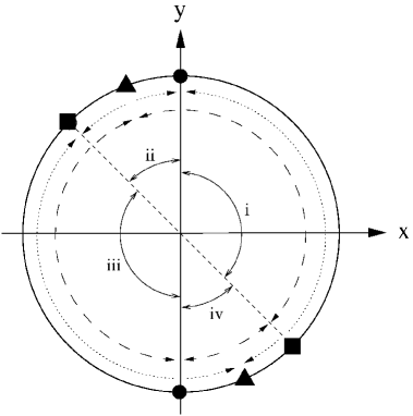
(b) The ($x$,$y$) plane when $-1<B<1/5$. Triangles now correspond to (39), and are located in the intervals ($-\pi/2$,$-\pi/4$) and ($\pi/2$,$3\pi/4$). The dashed arrows denote the direction of trajectories when $0<B<1/5$, and the dotted ones when $-1<B<0$.

Figure 1: The ($x$,$y$) plane in the phase space of vacuum solutions, defined by equations (14)-(16). The arrows indicate the trajectories of solutions, confined to the circle in each plot by the constraint equation, (17). Stationary points are indicated by dots, squares and triangles, and divide the phase space into the four sub-spaces $i$ to $iv$, between which trajectories cannot pass. Dots correspond to the points $1$ and $2$, and do not move. Squares correspond to points $3$ and $4$, and also do not move. The Triangles correspond to the critical points defined by (39), which can move. They approach the stationary points $5$ and $6$ in the limit $B\rightarrow B_{0}=$constant.

We now know the location and stability properties of all stationary points in the ($\theta$,$z$) phase space. The possible trajectories of solutions in this space can therefore be deduced, and are represented in the plots of Figure 1, which show slices through the ($x$,$y$) plane. Trajectories on these diagrams are confined to the black circles, and are separated into four sub-spaces by the circles and squares that denote $\theta_{1,2}$ and $\theta_{3,4}$, respectively. These four regions are labelled $i$ to $iv$, and trajectories that begin in one region are confined to that region for all $\tau$. The triangles correspond to the points

$$\tan\theta_{c}=\frac{2(2B-1)}{(B+1)}.$$ (39)

Other than points $1-4$, these are the only places at which $\theta^{\prime}$ can be momentarily zero. The triangles can move, as $R$ evolves, and in the limit $B\rightarrow B_{0}$ they approach the stationary points $5$ and $6$. Plot 1(a) corresponds to the cases $B<-1$ and $B>1/5$, when the triangles are in regions $i$ and $iii$. Plot 1(b) corresponds to $-1<B<1/5$, when they are in regions $ii$ and $iv$.

Let us first consider the cases depicted in Figure 1(a): $B<-1$ and $B>1/5$. In this figure the arrows show the direction of trajectories. Expanding cosmologies have $x>0$, and so are restricted to regions $i$ and $iv$. All trajectories in region $iv$ start at point $3$ and end at point $1$. The other expanding trajectories, in region $i$, begin at either point $2$ or point $3$, and all end on point $5$, if that point exists. If point $5$ does not exist then either $\theta_{c}$ is in perpetual motion in region $i$, or it moves out of region $i$ into either region $ii$ or $iv$. In the former case there is then no simple late-time attractor: trajectories are constantly evolving toward the moving $\theta_{c}$. In the latter case $B$ enters the interval $-1<B<1/5$, and the trajectories are simply attracted to either point $3$ or point $4$, as shown in Figure 1(b), and described below. The collapsing cosmologies with $x<0$, and described by trajectories in regions $ii$ and $iii$, can be seen to behave in a similar way, but with the direction of time reversed, and with points $2$ and $3$ inter-changed with points $1$ and $4$.

Now consider the cases in Figure 1(b): $-1<B<1/5$. The triangles are now found in regions $ii$ and $iv$. Here the dashed arrows show the direction of trajectories when $0<B<1/5$, and the dotted arrows show them for $-1<B<0$. First consider the former case, with $0<B<1/5$. Expanding cosmologies again have $x>0$, and so again must be confined to regions $i$ and $iv$. Now all trajectories in region $i$ begin at point $2$ and end at point $3$. Trajectories in region $iv$ are attracted to point $1$ or $3$ in the future, and in the past can be seen to approach $\theta_{c}$. If the stationary point $5$ exists, then trajectories in this region will approach it in the past. The collapsing cosmologies in regions $ii$ and $iii$, can again be seen to behave in a similar fashion to the expanding solutions, but with the direction of time reversed. The cases in which $-1<B<0$, depicted by dotted arrows, have exactly the opposite behaviour to the description just given. Past and future attractors must then be interchanged, but the description is otherwise the same.

Let us now consider further the asymptotic form of the scale factor as the stationary points are approached. The functional form of the scale-factor, $a(t)$, at points $5$ and $6$ has been determined above, and is given by (10). If

$$\frac{B_{5}(1+B_{5})}{(1-3B_{5}+2B_{5}^{2})}>0$$ (40)

then the late-time behaviour of the expanding point $5$ approaches a simple scaling solution as $t\rightarrow\infty$. If this condition on $B_{5}$ is not met, then in order to maintain $H>0$ it must be the case that $t<t_{0}$. In the limit that $t\rightarrow t_{0}$ the scale factor then diverges, and a big-rip singularity occurs. It can be seen that divergent behaviour occurs if $-1<B_{5}<0$, or $1/2<B_{5}<1$. This range of $B$ contains some interesting $f(R)$ theories, as we will show later on. Again, the behaviour of $a(t)$ as point $6$ is approached is similar, but with the direction of time reversed.

The points $3$ and $4$ have a simpler interpretation, as, independent of $B$, the scale factor evolves like a radiation dominated flat Friedmann universe when they are approached. Point $3$ always corresponds to an expanding universe. For $0<B<1/5$ this expanding solution is stable, and trajectories that are attracted toward it then approach the simple scaling behaviour (13) as $t\rightarrow\infty$. For $B<0$ or $B>1/5$ the expanding solution at $3$ is a repellor. Trajectories that originate from this point therefore have a big-bang singularity in their past, which they approach as $a\propto(t-t_{0})^{\frac{1}{2}}$ when $t\rightarrow t_{0}$. The collapsing trajectories corresponding to point $4$ have a similar interpretation, with the direction of time reversed.

Finally, consider the points $1$ and $2$, where $x/y\rightarrow 0$ and $1/y\rightarrow 0$. These points correspond to $a^{\prime}/a\rightarrow$0, which is either a stationary point in the evolution of $a(t)$, an approach to Minkowski space or a divergence in $R$. In order to determine which of these is the case it appears necessary to have a knowledge of the functional form of $f(R)$, so that equations (14)-(17) can be solved for in these limits. We can, however, make some progress in the cases in which $A_{1,2}$ and $B_{1,2}\rightarrow$constant. Equations (15), (16) and (17) can then be integrated to give

$$x \rightarrow\frac{1}{6}QB(1+A)(\tau-\tau_{0})$$ (41)

$$y \rightarrow\frac{1}{(1+A)(\tau-\tau_{0})}$$ (42)

$$z \rightarrow z_{0}+\frac{2A}{(1+A)}\ln(\tau-\tau_{0}),$$ (43)

where $\tau_{0}$ and $z_{0}$ are constants. The definition $d\tau=\sqrt{|R|}dt$ can also be integrated to give

$$(\tau-\tau_{0})\propto(t-t_{0})^{(1+A)}.$$ (44)

It can now be seen that $y\rightarrow\pm\infty$ corresponds to $\tau\rightarrow\tau_{0}$. For $A>-1$ this corresponds to $t\rightarrow t_{0}$, while for $A<-1$ it corresponds to $t\rightarrow\pm\infty$. The scale factor is now found to be

$$\ln\left(\frac{a}{a_{0}}\right)=(\tau-\tau_{0})^{2}\propto(t-t_{0})^{2(1+A)},$$ (45)

where $a_{0}$ is a constant. A solution that approaches $\theta_{1,2}$ with $A>-1$ reaches a stationary point in its expansion at a finite time, $t_{0}$. This solution must then be matched onto another solution with a similar stationary point in its past. If $A<-1$ as $\theta_{1,2}$ is approached, then these points are reached only as $t\rightarrow\infty$. These trajectories then approach Minkowski space asymptotically.

4 Perfect Fluid Cosmologies

4.1 The Dynamical System

Now consider the case $\rho\neq 0$ in equations (6)-(9). In this case we begin by transforming the time coordinate from $t$ to $T$ via

$$dT\equiv\sqrt{\frac{8\pi\rho}{3|f_{R}|}}dt,$$ (46)

where it has been assumed $\rho\geqslant 0$, so that $T$ is always real and increases monotonically in $t$. Defining the new variables $w\equiv\sqrt{|f_{R}||R|/8\pi\rho}$, $x\equiv a^{\prime}/a$, $y\equiv f_{R}^{\prime}/f_{R}$ and $z\equiv\ln|R|$ the equations (6)-(9) can then be written as

$$w^{\prime} =w\left(\left(\frac{1}{2}+A\right)y+\frac{3}{2}\gamma x\right)$$ (47)

$$x^{\prime} =\left(\frac{3}{2}\gamma-2\right)x^{2}+\frac{1}{2}xy+\frac{1}{2}Qw^{2}$$ (48)

$$y^{\prime} =\left(\frac{3}{2}\gamma+1\right)xy-\frac{1}{2}y^{2}-Qw^{2}-3\gamma S+4x^{2}$$ (49)

$$z^{\prime} =2Ay,$$ (50)

with the constraint equation

$$x^{2}+xy-\frac{1}{2}QBw^{2}-S=0,$$ (51)

where primes are now understood to denote differentiation with respect to $T$, and $Q$ and $S$ are the signs of $R$ and $f_{R}$, respectively. The functionals $A=A(z)$, and $B=B(z)$ are the same as before.

It can again be seen that the surfaces $R=0$ are invariant sub-manifolds of the phase space. These surfaces are now given by (51) as $x^{2}+xy-S=0$, and it can be seen that

$$(x^{2}+xy-S)^{\prime}=(x^{2}+xy-S)(3\gamma x+y/B),$$ (52)

showing that there exist no trajectories in this space along which $R$ changes sign, justifying our choice of $z$.

To find the stationary points, at finite distances in $x$ and $y$, we can eliminate $w$ using the constraint equation, (51). The dynamical system is then described by a three-dimensional closed system of equations, with four stationary points at finite distance in the ($x$,$y$) plane. These points are at

$$x_{7,8}=\frac{\pm\sqrt{S}}{\sqrt{5-3\gamma}}\qquad\qquad\qquad\qquad y_{7,8}=\pm\frac{(4-3\gamma)}{\sqrt{5-3\gamma}}\sqrt{S}$$ (53)

and

$$x_{9,10}=\frac{\pm\sqrt{2S}}{\sqrt{2-3\gamma B_{0}^{2}-B_{0}(4+3\gamma)}}\qquad\qquad y_{9,10}=\frac{\mp 3\gamma B_{0}\sqrt{2S}}{\sqrt{2-3\gamma B_{0}^{2}-B_{0}(4+3\gamma)}},$$ (54)

where the $\pm$ signs should be chosen consistently for each point, and where $B\rightarrow B_{0}=$constant. If the limit $B\rightarrow B_{0}=$constant does not occur, then points $9$ and $10$ do not exist. These points must also have real $x_{i}$ and $y_{i}$ in order to exist.

We will now find the form of the scale factor for the points $7$-$10$. From the definitions of $x$ and $y$ it is clear that at $x=x_{i}$ and $y=y_{i}$ we should have $f_{R}\propto e^{y_{i}(T-T_{0})}$, and $a\propto e^{x_{i}(T-T_{0})}$. The conservation equation (8) then yields $\rho\propto a^{-3\gamma}\propto e^{-3\gamma x_{i}(T-T_{0})}$, which, for $B\neq 1$, allows (46) to be integrated to

$$(t-t_{0})\propto e^{\frac{1}{2}(y_{i}+3\gamma x_{i})(T-T_{0})}.$$ (55)

The scale factor can then be written, as a function of $t$, in the power law form

$$a_{i}\propto(t-t_{0})^{\frac{2}{3\gamma+y_{i}/x_{i}}}.$$ (56)

At points $7$ and $8$ the scale factor can be seen to evolve like the Tolman solution, (13), while at points $9$ and $10$ it evolves like the matter dominated solution, (12). One may expect a different behaviour at these points when $B=1$, but for this value of $B$ points $9$ and $10$ do not exist for any positive $\gamma$.

Now consider stationary points at infinite distances in the ($x$,$y$) plane. To identify these points it is convenient to transform to polar coordinates via $x\equiv\hat{r}\cos\phi$ and $y\equiv\hat{r}\sin\phi$. Re-defining the radial coordinate as $\hat{r}\equiv r/(1-r)$ maps the infinite ($x$,$y$) plane to a unit disk, where $r\rightarrow 1$ in the limit $\hat{r}\rightarrow\infty$. In these coordinates equations (48) and (49) become

$$r^{\prime} =\frac{1}{4}\Big{[}(6\gamma-5)r^{2}\cos\phi-3\cos(3\phi)r^{2}-3(4\gamma S(1-r)^{2}-r^{2})\sin\phi$$

$$\qquad\qquad\qquad\qquad\qquad\qquad+5r^{2}\sin(3\phi)+2Q(1-r)^{2}(\cos\phi-2\sin\phi)w^{2}\Big{]}$$

$$\phi^{\prime} =\frac{1}{2r(1-r)}\Big{[}\cos\phi(3r^{2}-6\gamma S(1-r)^{2}+5r^{2}\cos(2\phi)$$

$$\qquad\qquad\qquad\qquad\qquad\qquad+3r^{2}\sin(2\phi))-Q(1-r)^{2}(2\cos\phi+\sin\phi)w^{2}\Big{]},$$

where $w$ is given by (51) as

$$w^{2}=\frac{(r^{2}-2S(1-r)^{2}+r^{2}\cos(2\phi)+r^{2}\sin(2\phi))}{BQ(1-r)^{2}}.$$ (57)

As $r\rightarrow 1$, and infinite distances in the ($x$,$y$) plane are approached, these equations become

$$r^{\prime} \rightarrow\frac{1}{4B}\Big{[}(1-(5-6\gamma)B)\cos\phi+3(1-B)\cos(3\phi)-(1-3B)\sin\phi-(1-5B)\sin(3\phi)\Big{]}$$ (58)

$$\phi^{\prime} \rightarrow-\frac{(1+\cos(2\phi)+\sin(2\phi))}{2B(1-r)}\Big{[}(1+B)\sin\phi+2(1-2B)\cos\phi\Big{]},$$ (59)

independent of the behaviour of $B$. It can now be seen from (59) that stationary points at infinite distances, as $r\rightarrow 1$, can exist only if $1+\cos(2\phi)+\sin(2\phi)=0$, or $\tan\phi=2(2B-1)/(B+1)$. This gives stationary points at

$$\phi_{1}=-\pi/2,\qquad\phi_{2}=\pi/2,\qquad\phi_{3}=-\pi/4,\qquad\phi_{4}=3\pi/4,$$ (60)

and at the two solutions of

$$\tan\phi_{5,6}=2(2B_{0}-1)/(B_{0}+1)$$ (61)

that exist in the range ($0$,$2\pi$). These points can be seen to be in similar positions to those in the vacuum cosmologies, and we will see that the scale factor evolves in a similar way as they are approached. Points $1$ to $4$ exist for any $B$, while $5$ and $6$ require $B\rightarrow B_{0}=$constant as they are approached, in order to be stationary.

To find the evolution of the scale factor at points $3$-$6$ we first see that the definitions of $x$ and $y$ allow an integral such that $f_{R}\propto a^{\tan\phi_{i}}$, just as in the vacuum FRW case. Substituting this into (48) and (49) allows us to obtain

$$\frac{a^{\prime\prime}}{a}\rightarrow\frac{((3\gamma+2)+\frac{3}{2}(2+\gamma)\tan\phi_{i}-\frac{1}{2}\tan^{2}\phi_{1})}{(2+\tan\phi_{i})}\frac{a^{\prime 2}}{a^{2}}-\frac{3\gamma S}{(2+\tan\phi_{i})}$$ (62)

as these points are approached. This equation can then be integrated to give

$$x^{2}=\frac{a^{\prime 2}}{a^{2}} =\frac{6\gamma S}{6\gamma+(4+3\gamma)\tan\phi_{i}-\tan^{2}\phi_{i}}+c_{1}a^{3\gamma+\tan\phi_{i}\frac{(4-\tan\phi_{i})}{(2+\tan\phi_{i})}}$$ (63)

$$\rightarrow c_{1}a^{3\gamma+\tan\phi_{i}\frac{(4-\tan\phi_{i})}{(2+\tan\phi_{i})}},$$ (64)

where the second line is in the limit $x^{2}\rightarrow\infty$, as is the case for all of points $3$-$6$. This equation can be integrated again, for $\tan\phi_{i}\neq 0$ or $1$, to find the form of the scale factor, as points $3$-$6$ are approached, to be

$$a \propto(T-T_{0})^{-\frac{2(2+\tan\phi_{i})}{(6\gamma+(4+3\gamma)\tan\phi_{i}-\tan^{2}\phi_{i})}}$$ (65)

$$\propto(t-t_{0})^{\frac{2\cot\phi_{i}+1}{\tan\phi_{i}-1}},$$ (66)

where $T_{0}$ and $t_{0}$ are constants of integration, and the second line has been obtained by an integration of equation (46), the definition of $T$. Substituting $\phi_{i}$ into the expression above shows that points $3$ and $4$ correspond to the Tolman solution, (13), and points $5$ and $6$ to the vacuum dominated solution, (10). This is as may have been expected by analogy to the vacuum cosmologies, investigated above. The special cases $\tan\phi_{i}=0$ and $1$, corresponding to points $5$ and $6$ when $B_{0}=1/2$ or $1$, give $a_{5,6}\propto\exp\{c(t-t_{0})\}$. Points $1$ and $2$ correspond to $a^{\prime}/a=0$.

The evolution of the scale factor at the stationary points $1$ to $10$ is summarised in Table 3. The symbols in this table refer to those used in Figures 2-6.

Point	a(t)	Symbol
1, 2	$a^{\prime}/a=0$	Circle
3, 4	Tolman solution, (13)	Square
5, 6	Vacuum dominated solution, (10)	Triangle
7, 8	Tolman solution, (13)	Square
9, 10	Matter dominated solution, (12)	Star

Table 3: The evolution of the scale factor, $a(t)$, at the critical points $1$-$10$ in perfect fluid filled $f(R)$ cosmologies. The listed symbols correspond to those used in Figures 2-6.

4.2 Stability Properties

Having found all stationary points, at both finite and infinite distances in the ($x$,$y$) plane, we will now proceed to establish their stability properties. This will allow some insight into the degree to which they can be considered the asymptotic limits of the general solutions to the Friedmann equations, (6) and (7).

First consider the points at finite distances in ($x$,$y$), points $7$-$10$. As these points are approached $z$ can be seen to diverge to $\pm\infty$. We can therefore check stability in the ($x$,$y$) plane by perturbing $x$ and $y$ as

$$x\rightarrow x_{i}+u\qquad\qquad\text{and}\qquad\qquad y\rightarrow y_{i}+v,$$ (67)

and checking the signs of the eigenvalues, $\lambda_{i}$, of the linearised equations

$$u^{\prime}=\lambda_{i}u\qquad\qquad\text{and}\qquad\qquad v^{\prime}=\lambda_{i}v.$$ (68)

Substituting (67) into (48) and (49) gives the linearised system

$$u^{\prime} =\frac{(2(2x_{i}+y_{i})+((6\gamma-8)x_{i}+y_{i})B)}{2B}u+\frac{x_{i}(2+B)}{2B}v$$ (69)

$$v^{\prime} =\frac{((16x_{i}+2y_{i}+3\gamma y_{i})B-4(2x_{i}+y_{i}))}{2B}u+\frac{(((2+3\gamma)x_{i}-2y_{i})B-4x_{i})}{2B}v,$$ (70)

where $B$ in these expressions is in the limit $R\rightarrow 0$ or $\infty$, whichever is appropriate. The eigenvalues, $\lambda_{i}$, are then given by the roots of a quadratic equation of the form $\lambda_{i}^{2}+\alpha\lambda_{i}+\beta=0.$ If $\alpha>0$ and $\beta>0$ we have a stable point in the ($x$,$y$) plane. If $\alpha<0$ and $\beta>0$ we have an unstable point, and if $\beta<0$ we have a saddle point. The behaviour of $z$ can be found by checking the sign of $z^{\prime}$. For points $7$ and $8$ we find that

$$\alpha=\mp\frac{((4-3\gamma)-(5-6\gamma)B)\sqrt{S}}{B\sqrt{5-3\gamma}}\qquad\qquad\text{and}\qquad\qquad\beta=-\frac{(4-3\gamma(1-B))S}{B},$$ (71)

where the branch of $\mp$ should be chosen consistently with equation (53). Similarly, for points $9$ and $10$ we find

$$\alpha=\mp\frac{3((1+B)\gamma-2)\sqrt{S}}{\sqrt{2(2-B(4+3\gamma(1+B)))}}\qquad\ \qquad\text{and}\qquad\qquad\beta=\frac{(4-3\gamma(1-B))S}{B},$$ (72)

with $\mp$ chosen consistent with (54). It can immediately be seen that one of these two sets of points always corresponds to a pair of saddles, as $\beta$ has opposite signs in (71) and (72). The other set can then be seen to contain one attractor and one repellor, as $\alpha$ has a different sign for each point in both (71) and (72). Which two points are saddles, which is the attractor and which is the repellor depends on the values of $B$, $\gamma$ and $S$. We will consider various cases below.

Now consider the stability of the stationary points at infinite distances in ($x$,$y$). In this case we perturb $\phi$ so that $\phi\rightarrow\phi_{i}+\delta\phi$. For points $1$ and $2$ we must also consider a perturbation to $z$ such that $z\rightarrow z_{i}+\delta z$, and $B\rightarrow B+(dB/dz)\delta z$. The evolution equation (58) and (59) then become

$$\delta\phi^{\prime}_{1,2}=\mp\frac{(1+B)}{(1-r)B}\delta\phi_{1,2}\qquad\qquad\text{and}\qquad\qquad r^{\prime}_{1,2}=\pm\frac{1}{2},$$ (73)

independent of $\delta z$. The upper sign here is for point $1$, and the lower sign for point $2$. These points are considered stable if $r^{\prime}>0$ and $\delta\phi/\phi<0$, unstable if $r^{\prime}<0$ and $\delta\phi/\phi>0$, and as saddle points otherwise. Therefore, if $B>0$ or $<-1$ then one of these points is stable and the other unstable. If $-1<B<0$ then both points are saddles.

For points $3$-$6$ both $r$ and $z\rightarrow\infty$, while $\phi$ is finite (for $B\neq 1/2$ or $1$). It is therefore sufficient to perturb $\phi$ as $\phi\rightarrow\phi_{i}+\delta\phi$, and to check the signs of $r$ and $z$. As $\phi\rightarrow\phi_{i}$, and $r\rightarrow\infty$, we then have for points $\phi_{3,4}$

$$\delta\phi^{\prime}_{3,4}=\mp\frac{(1-5B)}{\sqrt{2}B}\frac{\delta\phi_{3,4}}{(1-r)}\qquad\qquad\text{and}\qquad\qquad r^{\prime}_{3,4}=\mp\frac{(5-3\gamma)}{2\sqrt{2}},$$ (74)

where the upper sign is for $\phi_{3}$, and the lower sign for $\phi_{4}$. For points $5$ and $6$

$$\delta\phi^{\prime}_{5,6}=\pm\frac{(1-5B)}{B\sqrt{1+\frac{4(1-2B)^{2}}{(1+B)^{2}}}}\frac{\delta\phi_{5,6}}{(1-r)}\qquad\qquad\text{and}\qquad\qquad r^{\prime}_{5,6}=\mp\frac{(2-(4+3\gamma(1+B))B)}{2B(1+B)\sqrt{1+\frac{4(1-2B)^{2}}{(1+B)^{2}}}},$$ (75)

where the upper sign is for point $5$, and the lower for point $6$. It can be seen from the $\delta\phi$ equations that for $0<B<1/5$ the only points that can be stable are $3$ and $6$, and that the only points that can be unstable are $4$ and $5$. For $B<0$ or $B>1/5$ this behaviour is reversed and $4$ and $5$ are the only points that can be stable, while $3$ and $6$ are the only unstable points. The special cases $B=1/2$ and $1$ can have $z$ asymptoting to a finite value, and so in this case the stability analysis must include a perturbation to $z$. In Appendix A we perform this analysis, and find similar behaviour to the corresponding vacuum cosmologies investigated above.

The stability of the critical points $1$-$10$ can be seen to be strongly dependent on the value of the parameter $B$, as in the vacuum case. Now, however, the additional parameters $\gamma$ and $S$ are also involved in determining stability. The results for the different cases $S=\pm 1$, and $\gamma\gtrless 5/3$ are summarised in Tables 4-7. Having determined the stability properties of all stationary points, at both finite and infinite distances in the ($x$,$y$) plane, we will now proceed to investigate what this can tell us about the behaviour of the general solution.

Point	Stability when $\mathbf{S=-1}$ and $\mathbf{\gamma>5/3}$
	$\mathbf{B<-1}$	$\mathbf{-1<B<0}$	$\mathbf{0<B<1/5}$	$\mathbf{1/5<B}$
1	A	S	A	A
2	R	S	R	R
3	S	S	A	S
4	S	S	R	S
5	$m<0$: A	A	$m<0$: S	A
	$m>0$: S		$m>0$: R
6	$m<0$: R	R	$m<0$: S	R
	$m>0$: S		$m>0$: A
7	R	R	S	$n<0$: S
				$n>0$: R
8	A	A	S	$n<0$: S
				$n>0$: A
9	$m<0$: S	–	$m<0$: R	$n<0$: R
	$m>0$: –		$m>0$: –	$n>0$: S
10	$m<0$: S	–	$m<0$: A	$n<0$: A
	$m>0$: –		$m>0$: –	$n>0$: S

Table 4: The stability properties of the critical points $1$-$10$ in perfect fluid $f(R)$ cosmologies, when $S=-1$ and $\gamma>5/3$. Here ‘A’ denotes a stable Attractor, ‘R’ an unstable Repellor and ‘S’ a Saddle point. The quantities $m$ and $n$ are defined as $m\equiv 2-3\gamma B^{2}-B(4+3\gamma)$, and $n\equiv 3\gamma B^{2}+B(4-3\gamma)$. Dashes indicate that a point is not present for that range of $B$.

Point	Stability when $\mathbf{S=-1}$ and $\mathbf{0<\gamma<5/3}$
	$\mathbf{B<-1}$	$\mathbf{-1<B<0}$	$\mathbf{0<B<1/5}$	$\mathbf{1/5<B}$
1	A	S	A	A
2	R	S	R	R
3	R	R	S	R
4	A	A	S	A
5	$m<0$: A	A	R	$m<0$: A
	$m>0$: S			$m>0$: S
6	$m<0$: R	R	A	$m<0$: R
	$m>0$: S			$m>0$: S
7	–	–	–	–
8	–	–	–	–
9	$m<0$: S	–	–	$m<0$: S
	$m>0$: –			$m>0$: –
10	$m<0$: S	–	–	$m<0$: S
	$m>0$: –			$m>0$: –

Table 5: The stability properties of the critical points $1$-$10$ in perfect fluid $f(R)$ cosmologies, when $S=-1$ and $0<\gamma<5/3$. Here A, R, S, and $m$ are defined as in Table 4. Dashes again indicate the absence of a point.

Point	Stability when $\mathbf{S=1}$ and $\mathbf{\gamma>5/3}$
	$\mathbf{B<-1}$	$\mathbf{-1<B^{\ast}<0}$	$\mathbf{0<B<1/5}$	$\mathbf{1/5<B}$
1	A	S	A	A
2	R	S	R	R
3	S	S	A	S
4	S	S	R	S
5	$m<0$: A	A	$m<0$: S	A
	$m>0$: S		$m>0$: R
6	$m<0$: R	R	$m<0$: S	R
	$m>0$: S		$m>0$: A
7	–	–	–	–
8	–	–	–	–
9	$m<0$: –	$\;\text{A}^{\dagger}$	$m<0$: –	–
	$m>0$: A		$m>0$: S
10	$m<0$: –	$\;\text{R}^{\dagger}$	$m<0$: –	–
	$m>0$: R		$m>0$: S

Table 6: The stability properties of the critical points $1$-$10$ in perfect fluid $f(R)$ cosmologies, when $S=1$ and $\gamma>5/3$. A, R, S, and $m$ are defined as in Table 4. Dashes indicate the absence of a point. The $\dagger$ here indicates that these points have the indicated stability as long as $\gamma<2$. The $\ast$ indicates the range of $B$ for which, in this case, there exist regions of the phase space without either an attractor or a repellor.

Point	Stability when $\mathbf{S=1}$ and $\mathbf{0<\gamma<5/3}$
	$\mathbf{B<-1}$	$\mathbf{-1<B^{\ast}<0}$	$\mathbf{0<B<1/5}$	$\mathbf{1/5<B}$
1	A	S	A	A
2	R	S	R	R
3	R	R	S	R
4	A	A	S	A
5	$m<0$: A	A	R	$m<0$: A
	$m>0$: S			$m>0$: S
6	$m<0$: R	R	A	$m<0$: R
	$m>0$: S			$m>0$: S
7	$m<0$: S			S
	$m>0,n<0$: A	$n<0$: A	$n<0$: A
	$m>0,n>0$: S	$n>0$: S	$n>0$: S
8	$m<0$: S			S
	$m>0,n<0$: R	$n<0$: R	$n<0$: R
	$m>0,n>0$: S	$n>0$: S	$n>0$: S
9	$n<0$: S	$n<0$: S	$n<0$: S	$m<0$: –
	$n>0$: A	$n>0$: A	$n>0$: A	$m>0$: A
10	$n<0$: S	$n<0$: S	$n<0$: S	$m<0$: –
	$n>0$: R	$n>0$: R	$n>0$: R	$m>0$: R

Table 7: The stability properties of the critical points $1$-$10$ in perfect fluid $f(R)$ cosmologies, when $S=1$ and $0<\gamma<5/3$. A, R, S, and $m$ are defined as in Table 4. Dashes indicate the absence of a point.

4.3 The General Solution

The general solutions to the Friedmann equations (6)-(7) in the presence of a perfect fluid are more complicated than the vacuum case. The phase space of solutions is now, in general, three dimensional. Nevertheless, it is still possible to make progress in understanding the general solution.

As was previously noted, the surfaces $x^{2}+xy=S$ (corresponding to $R=0$) are invariant sub-manifolds of the phase space. This equation has two roots, describing two non-intersecting surfaces that separate the the phase space into three different regions, between which trajectories cannot cross. The shape of these regions depends on the sign of $S$, and is illustrated in Figures 2-6 by the grey and white areas. These plots show the ($x$,$y$) plane, and some representative trajectories within it, for various values of $\gamma$ and $B$. The left-hand plot, (a), in each of these figures corresponds to $S=-1$, and the right-hand plot, (b), to $S=1$.

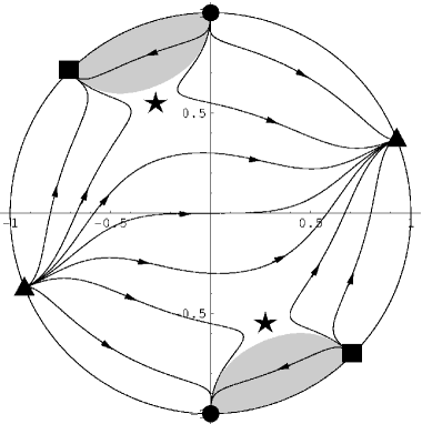
(a) $S=-1$

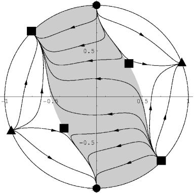
(b) $S=1$

Figure 2: The ($x$,$y$) plane in the phase space of solutions defined by equations (47)-(51). Here the infinite ($x$,$y$) plane has been compacted to a unit disk. Dots, squares, triangles and stars indicate the position of stationary points. Squares correspond to points $3$, $4$, $7$ and $8$, and hence the Tolman solution, (13). Stars correspond to points $9$ and $10$, and the matter dominated solution, (12). Triangles are at points $5$ and $6$, corresponding to the vacuum dominated solution, (10). Dots are at points $1$ and $2$, where $a^{\prime}/a=0$. The phase plane is separated into three different regions by the invariant sub-manifolds where $R=0$. Grey regions have $R<0$, and white regions have $R>0$. In these plots we take $B=2/3$ and $\gamma=1$, corresponding to pressureless dust and a gravitational Lagrangian dominated by a term $\sim R^{3}$.

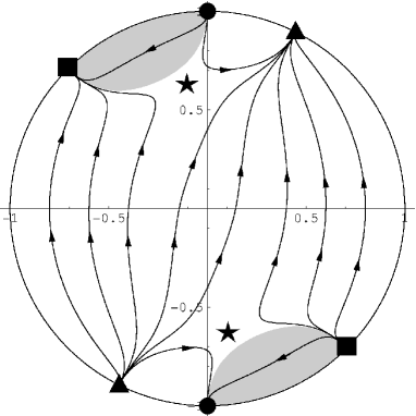
(a) $S=-1$

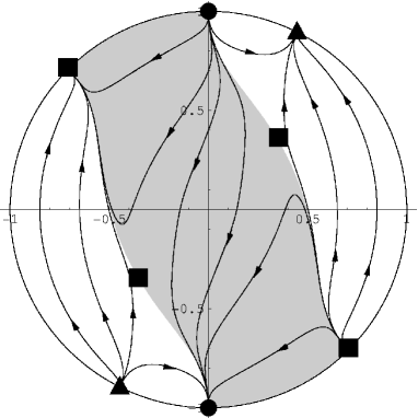
(b) $S=1$

Figure 3: These plots show the ($x$,$y$) plane in the phase space of solutions when $B=2$ and $\gamma=1$, corresponding to pressureless dust and a gravitational Lagrangian dominated by a term $\sim R^{-1}$. See the caption of Figure 2 for further details.

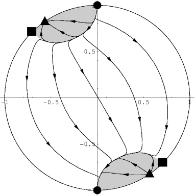
(a) $S=-1$

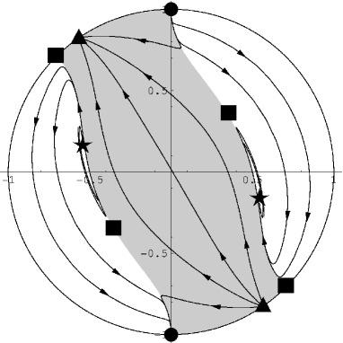
(b) $S=1$

Figure 4: Plots showing the ($x$,$y$) plane in the phase space of solutions when $B=1/10$ and $\gamma=1$, corresponding to pressureless dust and a gravitational Lagrangian dominated by a term $\sim R^{\frac{10}{9}}$. See the caption of Figure 2 for further details.

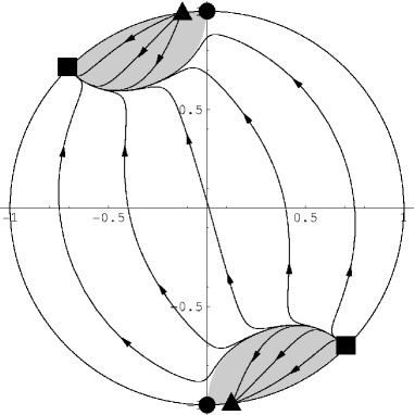
(a) $S=-1$

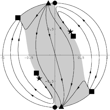
(b) $S=1$

Figure 5: Plots showing the ($x$,$y$) plane in the phase space of solutions when $B=-1/2$ and $\gamma=1$, corresponding to pressureless dust and a gravitational Lagrangian dominated by a term $\sim R^{\frac{2}{3}}$. See the caption of Figure 2 for further details.

A number of parallels can be drawn between the perfect fluid cosmologies, illustrated in Figures 2-6, and the vacuum cosmologies, illustrated in Figure 1. The circle at $r=1$ in Figures 2-6 can be seen to be quite similar to the circle in Figure 1. They both have stationary points at $\pi/2$ and $-\pi/2$, corresponding to $a^{\prime}/a=$constant, and at $-\pi/4$ and $3\pi/4$, corresponding to $a\sim t^{\frac{1}{2}}$ (although the coordinates have different definitions in each case). Whatsmore, in both cases these points mark the boundaries of regions between which trajectories cannot pass. A further similarity is in the position of the triangles, which correspond to the vacuum dominated solution, (10). In both cases, for $B>1/5$ or $<-1$, these points exist in what are labelled as region $i$ and $iii$ in Figure 1, and for $-1<B<1/5$, they exist in regions $ii$ and $iv$.

All of the points at $r=1$ therefore have analogous points in the vacuum cosmology case, and all of these points can be seen to exist for any $\gamma$, $B$ and $S$ (as long as $B\rightarrow B_{0}=$constant in the case of points $5$ and $6$). As $r$ increases these perfect fluid cosmologies therefore approach the behaviour of the vacuum cosmologies studied above. The principle difference between the perfect fluid case and the vacuum case is due to the existence of the extra dimension in the phase space. Points that were previously attractors (or repellors) in vacuo, can now be saddles in the presence of a perfect fluid, as they can be unstable (or stable) in the extra dimension. Whether these points maintain the attractor/repellor nature they exhibited in vacuo, or become saddles, can be read off from Tables 4-7.

As well as the points at $r=1$, there can exist four further points at finite distances in the ($x$,$y$) plane. These are points $7$-$10$, given by equations (53) and (54). They have no analogy in the vacuum cosmologies considered above, and do not exist for all $\gamma$, $B$ and $S$. Points $7$ and $8$ correspond to the Tolman solution, (13), and exist on the boundaries between grey and white regions. Points $9$ and $10$, correspond to the matter dominated solution (12), and can exist in either the grey or white regions. For $S=-1$ they are saddles if they exist in the the white region, and attractor/repellors if they exist in the grey regions. For $S=1$ this behaviour is reversed. If both of these sets of points exist then one of them will be a pair of saddle points, while the other will be an attractor/repellor pair. In general, the existence and stability of these points are functions of $\gamma$, $B$ and $S$, the details of which can be read off from Tables 4-7.

The existence, location and stability of the critical points, in the presence of a perfect fluid, is more complicated than the vacuum case. Rather than discuss all possible trajectories, we will therefore show a number of examples that we consider to be illustrative. In these examples $B$ will taken as a constant. It should be emphasised that in general $B$ is not a constant. However, for the purposes of illustrating the existence and attractor/repellor nature of the stationary points, for various different values of $B$, it is convenient to take it as so.

Figure 2 shows the ($x$,$y$) plane for a universe filled with pressureless dust, $\gamma=1$, for the case $B=2/3$. Such a value of $B$ may be expected if $f(R)\sim R^{3}$, and so may be of interest when higher powers of the curvature are expected to dominate the gravitational Lagrangian. Here the points at $r=1$ have locations and stability analogous to the vacuum case. There are also two points at finite distance, corresponding to the matter dominated solution, (12), when $S=-1$, and the Tolman solution, (13), when $S=1$. These points, however, are both saddles, and asymptotic behaviour in this case is therefore very similar to the corresponding vacuum cosmology.

Consider now the effect of lower orders of $R$ dominating the gravitational Lagrangian. If $f(R)\sim 1/R$ dominates then we may expect $B\rightarrow 2$. This case, with a dust equation of state, is illustrated in Figure 3. The asymptotes of the trajectories in Figure 3 can be seen to be very similar to those in Figure 2, and again the stability and location of the critical points are analogous to the corresponding vacuum cosmology. Only saddle points are introduced at finite distances in ($x$,$y$).

Let us now consider some ranges of $B$ for which we know the stability properties of the critical points to change. First consider $B$ in the range $0<B<1/5$, say $B=1/10$. This case would be expected from $f(R)\sim R^{\frac{10}{9}}$, and is shown in Figure 4, for $\gamma=1$. For $S=-1$ the points 3 and 4, at $-\pi/4$ and $3\pi/4$, are now no longer attractor/repellors, but saddle points. Trajectories that would otherwise have ended on them are now therefore drawn to points 1 and 2, at $-\pi/2$ and $\pi/2$. There are no new points at finite distances in this case, and the behaviour is otherwise the same as the corresponding vacuum cosmology. For $S=1$ points 3 and 4 are again saddles. Now, however, all four possible points at finite distances exist. The points 9 and 10 are now attractor/repellors, and so this case is qualitatively different from the corresponding vacuum cosmology, with new asymptotes possible. The case with $S=1$ is that which was considered in [17].

Another range of $B$ which we may wish to consider is $-1<B<0$, which is shown in Figure 5 for $B=-1/2$, corresponding to $f(R)\sim R^{\frac{2}{3}}$. The stability of the triangular points, corresponding to the vacuum solution (10), is now reversed, as would be expected from analogy with the vacuum cosmology. Now the circular points at $-\pi/2$ and $\pi/2$ are saddles, and the squares again have the attractor/repellor behaviour that would be expected from the corresponding vacuum cosmologies. The case $S=-1$ contains no extra critical points at finite distances, and so again has asymptotics that are otherwise the same as the vacuum case. For $S=1$ all four points at finite distances are present, and again points 9 and 10 act as attractor/repellors.

These examples have been intended to show some representative illustrations of the ($x$,$y$) phase plane, for different values of $B$. The figures shown above do not show all possible behaviours, and should not be considered exhaustive. It is, for example, quite possible to have points 7 and 8 acting as attractor/repellors, although this was not explicitly the case in any of the examples above. The reader will be able to find ranges of $B$ and $\gamma$ where this behaviour occurs, for either $S$, by referencing Tables 4-7, above.

It is of interest to note that for all but one configurations of $B$, $\gamma$ and $S$, there exists in each region of the ($x$,$y$) plane at least one attractor and one repellor. This is a necessary condition for there to exist no closed orbits, and for there to be at least one available attractor for each trajectory to end one, and one repellor from which it can begin. The exceptional case is $S=1$, $-1<B<0$ and $\gamma>5/3$. In this case there exist regions which are either without an attractor, or without a repellor. An example is shown in Figure 6. The star in the right-hand white region can be seen to act as an attractor, but following trajectories in this region backwards shows that they continue to spiral outwards forever. Such a trajectories therefore has no simple asymptote in the past. Similarly, in the left-hand white region of this plot all trajectories begin on the star, and spiral outwards forever as they are followed forward in time.

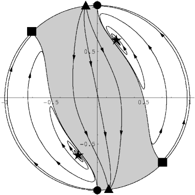
Figure 6: Plots showing the ($x$,$y$) plane in the phase space of solutions when $B=-1/2$, $S=1$ and $\gamma=2$. This situation corresponds to a stiff fluid and a gravitational Lagrangian dominated by a term $\sim R^{\frac{2}{3}}$. The left-hand white region in this plot has only a single repellor, and no attractor. Trajectories in this region can then be seen to originate from the repellor, but have no stable critical point to attract them in the future. They therefore spiral outwards forever, away from the repellor. The right-hand white region can similarly be seen to have an attractor but no repellor. See the caption of Figure 2 for further details.

Let us now consider further the behaviour of the scale factor, $a(t)$, as the critical points are approached. Trajectories approaching the points $1$-$6$ all have evolutions similar to those approaching the analogous points in the vacuum case. If condition (40) is met, then expanding trajectories with these points in their past all start with a big-bang singularity. Expanding trajectories that asymptote toward these points exhibit power-law behaviour, as $t\rightarrow\infty$. If condition (40) is not met, then expanding trajectories approaching points $5$ and $6$ have a big-rip singularity in their future.

The matter dominated points, $9$ and $10$, have no analogy in the vacuum cosmologies. Trajectories ending on these points approach the matter dominated solution (12). When $B<1$ these points correspond to a big bang in the past of expanding solutions, and to power-law expansion in their future. If $B>1$, for expanding solutions, then there is a big rip in the future, where $a\rightarrow\infty$ at finite $t$.

The two remaining points, $1$ and $2$, are at $y\rightarrow\pm\infty$, and $x/y\rightarrow 0$. In general it is required to solve the dynamical equation (47)-(51), for some particular $f(R)$, in order to find the form of $a(t)$ as these points are approached. If $A$ and $B\rightarrow$constant in this limit then (47)-(51) give

$$w \rightarrow w_{0}(T-T_{0})^{1+2A}$$ (76)

$$x \rightarrow\frac{1}{2}S(T-T_{0})+\frac{1}{4}QBw_{0}^{2}(T-T_{0})^{1+\frac{2}{B}}$$ (77)

$$y \rightarrow\frac{2}{(T-T_{0})}$$ (78)

$$z \rightarrow z_{0}+4A\ln(T-T_{0}),$$ (79)

where $T_{0}$, $w_{0}$ and $z_{0}$ are constants. The definition of $T$, (46), can then be integrated to

$$(t-t_{0})=\frac{\sqrt{3}w_{0}}{2e^{\frac{z_{0}}{2}}}(T-T_{0})^{2},$$ (80)

where $t_{0}$ is another constant. The limit $y\rightarrow\infty$ can now be seen to be reached as $T\rightarrow T_{0}$, and hence $t\rightarrow t_{0}$. The scale factor can then be found, by integrating $x$, to be

$$\ln\left(\frac{a}{a_{0}}\right) =\frac{1}{4}S(T-T_{0})^{2}+\frac{Qw_{0}^{2}B^{2}}{8(1+B)}(T-T_{0})^{\frac{2(1+B)}{B}}$$ (81)

$$=\frac{Se^{\frac{z_{0}}{2}}}{\sqrt{12}w_{0}}(t-t_{0})+\frac{Qw_{0}^{2}B^{2}}{8(1+B)}\left(\frac{2e^{\frac{z_{0}}{2}}}{\sqrt{3}w_{0}}\right)^{\frac{(1+B)}{B}}(t-t_{0})^{\frac{(1+B)}{B}}.$$ (82)

For $B>0$ or $B<-1$ the scale factor therefore reaches a finite value, $a_{0}$, as $t\rightarrow t_{0}$. The trajectory must then be matched onto another solution at this point, in order to make a complete history. If $-1<B<0$ then $a\rightarrow\infty$ as these points are approached, and there is a big rip as $t\rightarrow t_{0}$.

5 The Effect of Higher Powers

Most of the asymptotic behaviours found above correspond to scale factors obeying power laws of the form $a\sim(t-t_{0})^{k}$, where $k$ is some constant. In such cases the Ricci scalar is given by

$$R=\frac{6k(2k-1)}{(t-t_{0})}.$$ (83)

Solutions approaching these asymptotes, as $t\rightarrow\pm\infty$ or $t_{0}$, therefore have $R\rightarrow 0$ or $\pm\infty$. It is then straightforward to read off the values of $A$ and $B$ for different $f(R)$. Consider, for example, a theory of the type

$$f(R)=\sum_{i}c_{i}R^{i},$$ (84)

where the $c_{i}$ are constants, and the sum is over finite $i$. In this case the functions $A$ and $B$ are given by

$$A =\frac{\sum_{i}ic_{i}R^{i-1}}{2\sum_{j}j(j-1)c_{j}R^{j-1}}$$ (85)

$$B =\frac{\sum_{i}(i-1)c_{i}R^{i}}{\sum_{j}jc_{j}R^{j}}.$$ (86)

It can then be seen that as $R\rightarrow 0$, $A$ and $B$ approach the constant values

$$A\rightarrow\frac{1}{2(i_{-}-1)}\qquad\qquad\text{and}\qquad\qquad B\rightarrow\frac{(i_{-}-1)}{i_{-}},$$ (87)

where $i_{-}$ is the lowest power in $f(R)$. Similarly, as $R\rightarrow\pm\infty$ we have

$$A\rightarrow\frac{1}{2(i_{+}-1)}\qquad\qquad\text{and}\qquad\qquad B\rightarrow\frac{(i_{+}-1)}{i_{+}},$$ (88)

where $i_{+}$ is the highest power in $f(R)$. In such limits these theories behave as if $f(R)=R^{n}$, with the lowest power in (84) dominating as $R\rightarrow 0$, and the highest power dominating as $R\rightarrow\pm\infty$. Even in the absence of a highest power in $f(R)$ (that is, for an infinite power series) $A$ and $B$ can still approach constant values, a necessary condition to allow the existence of the vacuum dominated solutions, (10), and matter dominated solutions, (12).

The behaviour of $R$ at late times, and hence the possible asymptotic behaviour of $a(t)$, can now be determined from the behaviour of $R$ in that limit. If the vacuum dominated evolution (10) is approached, as often is the case, then this behaviour can be read off from condition (40). For $1/2<B<1$ we have at late times that $t\rightarrow t_{0}$, which corresponds to $R\rightarrow\pm\infty$ and, therefore, the asymptotic behaviour of $a(t)$ being dominated by the highest power of $R$ in the Lagrangian. This range of $B$ corresponds to a power $R^{n}$ with $n>2$. Conversely, for $B>1$ or $<-1$ we have that $t\rightarrow\infty$ at late times, so that $R\rightarrow 0$, and there can exist an asymptote in which $a(t)$ is dominated by the lowest power of $R$. These ranges of $B$ correspond to $R^{n}$ with $n<1/2$. If a theory contains a low power of $R$ in its Lagrangian there can then exist a vacuum dominated asymptote where $R\rightarrow 0$, and in which the lowest power of $R$ dominates. However, if that same theory contains high powers of $R$ in its Lagrangian there can also exist an asymptote where $R\rightarrow\infty$, and in which the highest power of $R$ dominates. Theories with multiple powers of $R$ can therefore have their late-time asymptotics dominated by either the lowest or highest power of $R$.

To illustrate these points further will now consider some example theories.

5.1 Adding Higher Powers to General Relativity

Consider adding to the Einstein-Hilbert action higher powers of $R$, such as $R^{2}$ and $R^{3}$. Such modifications have often been considered as possible UV ‘corrections’ to gravity, motivated by attempts to construct a perturbatively re-normalisable quantum field theory of gravity. It is frequently assumed that these higher-order ‘corrections’ to gravity should dominate the earliest stages of the Universe’s evolution. Let us investigate this possibility in the frame-work that has been constructed above.

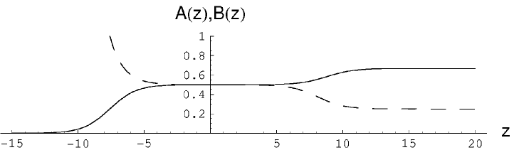
Figure 7: The functions $A(z)$ and $B(z)$ for the theory $f(R)=R+10^{3}R^{2}+0.1R^{3}$. The dashed line corresponds to $A$, and the solid line to $B$.

Figure 7 shows the functions $A(z)$ and $B(z)$ when $f(R)=R+10^{3}R^{2}+0.1R^{3}$. The dashed line in this plot is $A$, and the solid line is $B$. One can see the linear term dominates at low $R$, the quadratic term at intermediate $R$, and the cubic term at high $R$.

Consider a trajectory in the ‘high-curvature’ regime, $z\gtrsim 12$, so that $B\simeq 2/3$. In this case the stability of the various critical points, and their locations, are shown in Figure 2. The only expanding attractor is the vacuum dominated solution, (10), which in this case corresponds to $a\sim(t-t_{0})^{-10}$. As this attractor is approached we have $z^{\prime}>0$, so trajectories are pushed further into the the high $R$ regime, and toward an eventual big rip. For a trajectory at high-curvature to find its way down into the intermediate curvature regime, where $R^{2}$ dominates, it must therefore be either collapsing, or possibly in the early transient stages before an asymptotic attractor is approached.

Now consider a trajectory in the $R^{2}$ dominated regime, $-3\lesssim z\lesssim 5$, where $B\simeq 1/2$. The ($x$,$y$) plane looks very similar to Figure 2 in this case, but with the vacuum dominated points $5$ and $6$ displaced a little. Again, the only expanding attractor is the vacuum dominated solution, which in this case corresponds to exponential expansion, (26). This point is then semi-stable, in the sense described in Appendix A. Here we have $AB_{,z}>0$, so the vacuum dominated exponential expansion will eventually end with the point becoming a saddle in the phase space. Trajectories can then move to the higher or lower $R$ regimes.

The picture of a universe starting off expanding with the highest power in $f(R)$ dominating, and moving successively down through lower powers of $R$ until $f\sim R$ is reached does not appear to be a generic situation. In fact, if a higher power of $R$ (other than $R^{2}$) dominates the gravitational dynamics, then it appears that expanding trajectories are generically forced to higher $R$, rather than lower. The $R^{2}$ case is exceptional, and in this case expanding vacuum dominated trajectories do appear able to move to the lower $R$ regime, although even in this case it does not seem generic.

5.2 General Relativity as a Higher Power

Consider now a gravitational Lagrangian with an Einstein-Hilbert term, and both higher and lower powers of $R$. Lower powers of $R$ have been of interest recently, as they can correspond to cosmologies that accelerate at late times.

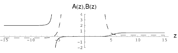
Figure 8: The functions $A(z)$ and $B(z)$ for the theory $f(R)=R+10^{-5}/R+10^{-5}R^{3}$. The dashed line corresponds to $A$, and the solid line to $B$.

In Figure 8 we show the form of $A(z)$ and $B(z)$ for the theory $f(R)=R+10^{-5}/R+10^{-5}R^{3}$. At high $R$ the $R^{3}$ term dominates, at intermediate $R$ the Einstein-Hilbert term dominates, and at low $R$ the inverse power, $1/R$, dominates. As before, when $R^{3}$ dominates the only expanding attractor at late times corresponds to increasing $R$. So again, only contracting solutions, or trajectories in the early transient stages, can make it down to the lower curvature regimes. A solution in the intermediate curvature regime, $-3\lesssim z\lesssim 3$, is dominated here by the Einstein-Hilbert term, with $B\simeq 0$. In this case the dynamical equations reduce to the usual Friedmann ones, and so $R$ decreases for expanding solutions, allowing for a transition to the $1/R$ regime, $z\lesssim-12$, where $B\simeq 2$.

The stability properties and location of critical points in the $1/R$ regime are shown in Figure 3. In this situation we again have that the only expanding attractor is the vacuum dominated solution, (10). In this case, however, $A<0$, so this attractor corresponds to decreasing $R$. Trajectories asymptoting toward this point are then pushed further and further into the $1/R$ dominated regime. If we were to have included an even lower power of $R$, say $1/R^{2}$, then expanding solutions heading toward the attractor solution would be pushed toward the regime in which this power dominates.

Expanding solutions in regimes dominated by the Einstein-Hilbert term, or lower powers of $R$, generically appear to move to lower and lower $R$ as they continue to expand. The term $R^{2}$ then acts as a watershed: expanding universes dominated by higher powers of $R$ appear to evolve toward higher $R$, while expanding universes dominated by lower powers move to lower $R$. For the case of high $R$ this corresponds to divergent expansion toward a big rip, and for low $R$ it corresponds to (possibly accelerating) eternal expansion.

5.3 Infinite Power Series

Having considered the case of single higher or lower powers dominating the gravitational Lagrangian, let us now consider infinite power series. There are, of course, very many functional forms that one may choose for $f(R)$ to illustrate the case of an infinite power series. Here we consider $f(R)=(R+100R^{3})e^{10^{-5}R}$. The corresponding functions $A(z)$ and $B(z)$ are shown in Figure 9. It can be seen that there are three different regimes: low $R$ at $z\lesssim-5$, where the Einstein-Hilbert term dominates with $B\simeq 0$, intermediate $R$ at $0\lesssim z\lesssim 10$, where $R^{3}$ dominates with $B\simeq 2/3$, and high $R$ at $z\gtrsim 15$, where the exponential dominates with $B\simeq 1$.

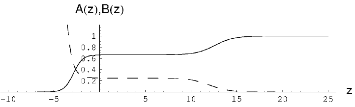
Figure 9: The functions $A(z)$ and $B(z)$ for the theory $f(R)=(R+100R^{3})e^{10^{-5}R}$. The dashed line corresponds to $A$, and the solid line to $B$.

The high $R$ regime now corresponds to $B\simeq 1$, which is one of the special cases in Appendix A. The vacuum dominated point $5$ is again the only expanding attractor, and now this point corresponds to exponential growth of the scale factor, as in (26). This point is then stable, as $A_{z}\leqslant 0$, but with $z^{\prime}=0$. While it can be the case that single higher powers dominate at intermediate regimes ($R^{3}$ in the region $0\lesssim z\lesssim 10$, here), the solutions heading toward the expanding attractor in such regimes are forced to higher $R$. The highest $R$ regime here, however, is at $B\simeq 1$. The late-time attractor then no longer corresponds to a big rip, but to exponential expansion, with $R\rightarrow$constant, instead of $\infty$. The behaviour of infinite power series in $R$ is therefore qualitatively different to the finite series considered previously. As before, only collapsing solutions, or possibly those in the early transient stages of their evolution, appear able to make it down to the low curvature regime.

6 Discussion

We have considered in this paper the evolution of spatially flat FRW universes governed by $f(R)$ theories of gravity. The Friedmann equations (6)-(8) were transformed into an autonomous system of first-order differential equations, and a dynamical systems analysis was performed. The location and stability of all critical points in the phase space were found, for both vacuum and perfect fluid cosmologies, and for general $f(R)$. It was shown that the simple power-law solutions, given by equations (10)-(13), often act as the early and late-time asymptotes of the general solution.

The general behaviour of $f(R)$ FRW cosmologies is complicated. The phase space of solutions is often divided into sub-spaces by invariant manifolds, through which the trajectories describing the general solution cannot pass. The asymptotic past of general solutions can contain points of inflexion, or big-bang singularities that can be approached in different ways. Similarly, future behaviour can be seen to be able to asymptote toward matter dominated expansion, (12), vacuum domination, (10), or various other forms. Whatsmore, the three dimensional phase space of solutions, in the presence of a perfect fluid, allows for the possible existence of strange attractors, and chaotic behaviour.

Nevertheless, despite the complicated behaviour exhibited by the general solutions, it is still possible to make statements about the effects of modifying the Einstein-Hilbert action to more general functions of $R$. It can be said that theories that contain lower powers of $R$ often have a stable asymptote that corresponds to the expanding vacuum dominated solution, (10), of that lowest power, and that therefore behave as if governed by a gravitational Lagrangian of the form (2) at late times. However, if a theory contains any higher powers of $R$ then there is also often a stable asymptote that corresponds to the expanding vacuum dominated solution, (10), of that highest power, and that therefore behaves as if governed by a Lagrangian of the form (3) at late times. Theories containing both higher and lower powers of $R$ can then asymptote, at late times, to regimes in which either the lowest or highest powers or $R$ dominate. In either case the consequent evolution is that of a gravitational Lagrangian dominated by a single power of $R$.

Which solutions asymptote to high $R$ domination, and which to low $R$ domination, depends on the initial conditions, and the form of $f(R)$. Using illustrative examples we have shown that if a power of $R$ higher than $R^{2}$ dominates at some point then the generic behaviour of expanding solutions is to higher $R$. If a power of $R$ lower than $R^{2}$ dominates, then the trend is to lower $R$. A term $R^{2}$ in the Lagrangian is then a special case; if it dominates then the expanding attractor corresponds to exponential growth, and acts as a separatrix between the higher or lower powers of $R$ dominating the future dynamics of the Universe. Those solutions with low $R$ dominating at late-times expand eternally, while those with high $R$ dominating approach either a big-rip singularity, or exponential expansion. Big-rips often occur if there exists a single power of $R$ that dominates at late times, and exponential expansion occurs if $B\rightarrow 1$, as is the case for some infinite power series, such as $f\sim\exp\{R\}$. This late-time acceleration does not appear to be a good candidate for the apparent acceleration we observe, however, as it cannot follow from a period of Einstein-Hilbert domination in which $R\rightarrow 0$.

The asymptotic past of the general solutions is similarly complicated. A variety of behaviours seems possible, including big-bang singularities and bounces, where the scale factor reaches a non-zero minimum. Big-bang singularities are often approached with the scale-factor behaving as in the Tolman solution, (13). It is interesting to note that even trajectories which undergo an early period of inflation (such as those solutions in which a power of $R^{2}$ dominates at some point) do not generically follow such expansion indefinitely into the past, but rather have a big bang or bounce at some point in their past, prior to the onset of inflation.

While the behaviour found here is quite complicated, with numerous different asymptotes possible, it is certainly not the most general case that one may consider. We have limited ourselves here to spatially flat FRW universes. Relinquishing the criterion of spatial flatness would lead to more complicated behaviours still, and one may also consider inhomogeneous and/or anisotropic cosmologies, or cosmologies with multiple fluids. It is not clear whether or not the behaviour identified above would hold in these more general cases or not. What does seem clear, however, is that the simple picture of the highest powers of $R$ dominating at early times, and lower powers dominating at late times, is unlikely to be accurate.

Appendix A Stability of ‘Vacuum Dominated’ Solutions when $\mathbf{B=1/2}$ or $\mathbf{1}$

When $B=1/2$ or $1$ the vacuum dominated solutions take an exponential form $a\sim e^{c(t-t_{0})}$, instead of the usual power-law form, (10). In this case the parameter $z=\ln|R|$ does not diverge to $\pm\infty$, and so the stability analysis must be modified from the power-law case. We will investigate the stability of these solutions here.

A.1 Vacuum Cosmologies

In the vacuum cosmologies, considered in section 3, points $5$ and $6$ correspond to exponential expansion when $B\rightarrow 1/2$ or $1$. Consider first the case $B\rightarrow 1/2$. Perturbing $\theta\rightarrow\theta+\delta\theta$ and $z\rightarrow z+\delta z$ we then have that the evolution equations (19) and (20) are, to linear order,

$$\delta\theta^{\prime} =\mp\frac{\sqrt{3Q}}{2}\delta\theta\pm\frac{4\sqrt{Q}}{\sqrt{3}}B_{,z}\delta z$$ (89)

$$\delta z^{\prime} =\pm A\sqrt{\frac{Q}{3}}\delta\theta,$$ (90)

where the upper branch corresponds to point $5$, and the lower branch to point $6$. It can now be seen that the eigenvalues to the equations $\delta z^{\prime}=\lambda_{i}\delta z$ and $\delta\theta^{\prime}=\lambda_{i}\delta\theta$ are given by the two roots of

$$\lambda_{i}^{2}\pm\frac{\sqrt{3Q}}{2}\lambda_{i}-\frac{4}{3}AB_{,z}Q=0.$$ (91)

On recognising that these solutions have $Q=1$, it can be seen that if $AB_{,z}>0$ then both points are saddles. Alternatively, if $AB_{,z}<0$ then point $5$ is stable, while point $6$ is unstable. We will also be interested in the case when $B_{,z}\simeq 0$. Point $5$ is then stable in $\theta$, while $\delta z^{\prime}=0$. Small fluctuations (as one would expect to occur in a thermal de Sitter space such as this) will then gradually shift the value of $z$. Unless the theory has $B_{,z}=0$ for all $z$, there will then come a time at which $B_{,z}\neq 0$, after which the point becomes an attractor proper, or a saddle, depending on the sign of $AB_{,z}$. We will refer to this situation of temporary stability, followed by saddle behaviour, as ‘semi-stable’.

Now consider the case $B\rightarrow 1$. In this case it is instructive to use the definitions of $A$ and $B$ to see that

$$A=\frac{(1-B)}{2(B+B_{,z})}.$$ (92)

For $B_{,z}\neq-1$ we then have that $B\rightarrow 1$ corresponds to $A\rightarrow 0$. Perturbing $\theta$ and $z$, as before, we then find that the linearised evolution equations become

$$\delta\theta^{\prime} =\mp 2\sqrt{\frac{Q}{3}}\delta\theta\pm\frac{\sqrt{3Q}}{2}B_{,z}\delta z$$ (93)

$$\delta z^{\prime} =\sqrt{\frac{Q}{3}}A_{,z}\delta z,$$ (94)

so that the relevant eigenvalues are given as the roots of

$$\lambda_{i}^{2}\pm\sqrt{\frac{Q}{3}}(2-A_{,z})\lambda_{i}-\frac{2}{3}A_{,z}Q=0.$$ (95)

Again, $Q=1$, so the condition for points $5$ and $6$ to be saddles is now $A_{,z}>0$. If $A_{,z}<0$ then point $5$ is an attractor, and point $6$ a repellor. Now, if $A_{,z}=0$, then point $5$ can be semi-stable, depending on the sign of $A_{z}$.

A.2 Perfect Fluid Cosmologies

In the perfect fluid cosmologies we also find that the vacuum dominated solution corresponds to exponential expansion when $B\rightarrow 1/2$ or $1$. Consider first the case $B\rightarrow 1/2$. In this case a perturbative expansion in $\phi$ and $z$ gives the evolution equations (50), (58) and (59), to linear order, as

$$\delta\theta^{\prime} =\pm\frac{(8B_{,z}\delta z-3\delta\theta)}{(1-r)}$$ (96)

$$\delta z^{\prime} =\pm\frac{(2A\delta\theta)}{(1-r)}$$ (97)

$$r^{\prime} =\pm\frac{3\gamma}{2},$$ (98)

where the upper sign is for point $5$ and the lower sign for point $6$. We are now looking for eigenvalues, $\lambda_{i}$, such that

$$\delta\theta^{\prime}=\frac{\lambda_{i}}{(1-r)}\delta\theta\qquad\qquad\text{and}\qquad\qquad\delta z^{\prime}=\frac{\lambda_{i}}{(1-r)}\delta z.$$ (99)

If both of these eigenvalues are negative, and $r^{\prime}>0$, then the point is stable. If they are both positive, and $r^{\prime}<0$, then the point is unstable. Any other combination we will call a saddle point. The values of $\lambda_{i}$ can be seen to be given by the roots of

$$\lambda_{i}^{2}\pm 3\lambda_{i}-16AB_{,z}=0.$$ (100)

It can then be seen that for $AB_{,z}>0$ both points are saddles, while for $AB_{,z}<0$ point $5$ is stable and point $6$ is unstable. $AB_{,z}=0$ again corresponds to point $5$ being semi-stable. The stability properties of points $5$ and $6$ in the presence of a perfect fluid when $B\rightarrow 1/2$ are therefore identical to the corresponding points in the vacuum cosmologies, considered above.

Finally, consider the case $B\rightarrow 1$. Equation (92) shows that in this limit we again have $A\rightarrow 0$. The perturbed evolution equations are then given as

$$\delta\theta^{\prime} =\pm\frac{(3B_{,z}\delta z-4\delta\theta)}{\sqrt{2}(1-r)}$$ (101)

$$\delta z^{\prime} =\pm\frac{\sqrt{2}A_{,z}\delta z}{(1-r)}$$ (102)

$$r^{\prime} =\pm\frac{\sqrt{2}}{4}(1+3\gamma),$$ (103)

where upper signs correspond to point $5$, and lower signs to point $6$. The eigenvalues, $\lambda_{i}$, are now given by the roots of

$$\lambda_{i}^{2}\pm\sqrt{2}(2-A_{,z})\lambda_{i}-4A_{,z}=0.$$ (104)

For $A_{,z}>0$ both of points $5$ and $6$ are saddles, while for $A_{,z}<0$ point $5$ is stable and point $6$ is unstable. $A_{,z}=0$ gives point $5$ as semi-stable. Again, the stability properties of these points is identical to the analogous points in the vacuum cosmologies.

Acknowledgements

I would like to thank John Barrow for suggestions, and to acknowledge the support of Jesus College, Oxford.

References

- [1] H. Buchdahl, J. Phys. A 12, 1229 (1979).
- [2] R. Kerner, Gen. Rel. Grav. 14, 453 (1982).
- [3] J. D. Barrow and A. C. Ottewill, J. Phys. A 16, 2757 (1983).
- [4] G. Magnano, M. Ferraris and M. Francaviglia, Gen. Rel. Grav. 19, 465 (1987).
- [5] E. Pechlaner and R. Sexl, Comm. Math. Phys. 2, 165 (1966).
- [6] M. Gasperini, M. Maggiore and G. Veneziano, Nucl. Phys. B 494, 315 (1997).
- [7] K. A. Meissner, Phys. Lett. B 392, 298 (1997).
- [8] S. M. Carroll, A. De Felice, V. Duvvuri, D. A. Easson, M. Trodden, and M. S. Turner, Phys. Rev. D 71, 063513 (2005).
- [9] S. Nojiri and S. D. Odintsov, Phys. Rev. D 68, 123512 (2003).
- [10] A. Berkin, Phys. Rev. D 44, 1020 (1991).
- [11] E. Bruning, D. Coule and C. Xu, Gen. Rel. Grav. 26, 1197 (1994).
- [12] J. D. Barrow and S. Hervik, Phys. Rev. D 73, 023007 (2006).
- [13] J. D. Barrow and J. Middleton, Phys. Rev. D 75, 123515 (2007).
- [14] J. D. Barrow and T. Clifton, Class. Quant. Grav. 23, L1 (2006).
- [15] T. Clifton and J. D. Barrow, Class. Quant. Grav. 23, 2951 (2006).
- [16] T. P. Sotiriou and V. Faraoni, arXiv:0805.1726 (2008).
- [17] T. Clifton and J. D. Barrow, Phys. Rev D 72, 103005 (2005).
- [18] S. Carloni, P. K. S. Dunsby, S. Capoziello and A. Troisi, Class. Quant. Grav. 22, 4839 (2005).
- [19] M. Abdelwahab, S. Carloni and P. K. S. Dunsby, Class. Quant. Grav. 25, 135002 (2007).
- [20] J. A. Leach, S. Carloni and P. K. S. Dunsby, Class. Quant. Grav. 23, 4915 (2006).
- [21] N. Goheer, J. A. Leach and P. K. S. Dunsby, Class. Quant. Grav. 24, 5689 (2007).
- [22] J. D. Barrow and S. Hervik, Phys. Rev. D 74, 124017 (2006).
- [23] T. Clifton, Class. Quant. Grav. 24, 5073 (2007).
- [24] L. Amendola, R. Gannouji, D. Polarski and S. Tsujikawa, Phys. Rev. D 75, 083504 (2007).
- [25] S. Carloni, A. Troisi and P. K. S. Dunsby, arXiv:0706.0452 (2007).
- [26] T. Clifton, Class. Quant. Grav. 23, 7445 (2006).
- [27] T. Clifton, Phys. Rev. D 77, 024041 (2008).