Equilibrium long-ranged charge correlations at the surface
of a conductor coupled to the electromagnetic radiation

Abstract

This study is related to the fluctuation theory of electromagnetic fields, charges and currents. The three-dimensional system under consideration is a semi-infinite conductor, modeled by the jellium, in vacuum. In previous theoretical studies it was found that the correlation functions of the surface charge density on the conductor decay as the inverse cube of the distance at asymptotically large distances. The prefactor to this asymptotic decay was obtained in the classical limit and in the quantum case without retardation effects. To describe the retarded regime, we study a more general problem of the semi-infinite jellium in thermal equilibrium with the radiated electromagnetic field. By using Rytov’s fluctuational electrodynamics we show that, for both static and time-dependent surface charge correlation functions, the inclusion of retardation effects causes the quantum prefactor to take its universal static classical form, for any temperature.

I Introduction

Experimental and theoretical investigations of charged systems in thermal equilibrium play a key role in the understanding of various fundamental properties of solids and liquids, in the bulk as well as on the surface. There exist two complementary theoretical approaches to Coulomb models: one based on the solution of microscopic models, the other based on the assumption of validity of macroscopic electrodynamics. The microscopic description is more laborious and complicated but, if available, it can reveal restricted applicability of the macroscopic theory. On the other hand, the macroscopic phenomenology usually allows us to predict, with much less effort, basic features of relatively complicated complex physical systems.

In this paper, we study the fluctuations of electromagnetic fields, charges and currents in systems formulated in the three-dimensional (3D) Cartesian space of points ${\bf r}=(x,y,z)$. We shall deal with semi-infinite geometries, inhomogeneous say along the first coordinate $x$. It will be sometimes useful to denote the remaining two coordinates normal to $x$ as ${\bf R}=(y,z)$. The physical situation we are interested in is pictured in Fig.1. In its most general formulation, the model consists of two semi-infinite media with the frequency-dependent dielectric functions $\epsilon_{1}(\omega)$ and $\epsilon_{2}(\omega)$, in the half-space $\Lambda_{1}=\{{\bf r}=(x,{\bf R});x>0\}$ and in the complementary half-space $\Lambda_{2}=\{{\bf r}=(x,{\bf R});x<0\}$, respectively. The interface between the media is localized at $x=0$. Although we shall derive basic formulas for this general case, the analysis of the results will be done for the specific case when the half-space $\Lambda_{1}$ is occupied by a Coulomb fluid, namely a jellium, and the half-space $\Lambda_{2}$ is formed by an impenetrable plain hard wall with the vacuum permittivity. For a Coulomb fluid composed of charged particles, the average particle density is varying at microscopic distances (of the order of the correlation length) from the interface. Since we shall be interested in macroscopic electrodynamic phenomena at distances much larger than the microscopic length scale, we can assume that the Coulomb fluid and the dielectric function are homogeneous in the whole half-space $\Lambda_{1}$.

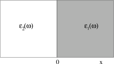
Figure 1: Two semi-infinite media characterized by dielectric functions $\epsilon_{1}(\omega)$ and $\epsilon_{2}(\omega)$.

The presence of the Coulomb fluid gives rise to a surface charge density $\sigma$ on the conductor which has to be understood as being the microscopic volume charge density integrated on some microscopic depth. It is associated with the discontinuity of the electric field ${\bf E}$ at the surface $x=0$ of the conductor. At a point ${\bf r}=(0,{\bf R})$ on the surface, in Gauss units,

$$4\pi\sigma({\bf R})=E_{x}^{+}({\bf R})-E_{x}^{-}({\bf R}),$$ (1)

where the upperscript $+$ $(-)$ means approaching the surface through the limit $x\to 0^{+}$ ($x\to 0^{-}$). The quantity of interest is the surface charge density correlation function between two points

$$\langle\sigma({\bf R})\sigma({\bf R}^{\prime})\rangle^{\rm T}=\frac{1}{(4\pi)^{2}}$$

$$\qquad\times\left\langle\left[E_{x}^{+}({\bf R})-E_{x}^{-}({\bf R})\right]\left[E_{x}^{+}({\bf R}^{\prime})-E_{x}^{-}({\bf R}^{\prime})\right]\right\rangle^{\rm T},\quad$$ (2)

where $\langle\cdots\rangle^{\rm T}$ represents a truncated equilibrium statistical average, $\langle AB\rangle^{\rm T}=\langle AB\rangle-\langle A\rangle\langle B\rangle$, at the inverse temperature $\beta$. The system is translationally invariant in the ${\bf R}$-plane and so the charge correlation function depends only on the distance between the points,

$$\langle\sigma({\bf R})\sigma({\bf R}^{\prime})\rangle^{\rm T}=S(|{\bf R}-{\bf R}^{\prime}|).$$ (3)

It is useful to introduce the Fourier transform

$$S({\bf q})=\int d^{2}R\,e^{i{\bf q}\cdot{\bf R}}S({\bf R}),$$ (4)

with ${\bf q}=(q_{y},q_{z})$ being the 2D wave vector.

For classical Coulomb fluids composed of charged particles with the instantaneous Coulomb interactions, $S(R)$ can be retrieved by simple macroscopic argument based on the electrostatic method of images, giving Jancovici (1995)

$$\beta S_{\rm cl}(R)=-\frac{1}{8\pi^{2}}\frac{1}{R^{3}},$$ (5)

where the distance $R=|{\bf R}|$ is much larger than any microscopic length scale, like the particle correlation length. Since, in the sense of distributions, the 2D Fourier transform of $1/R^{3}$ is $-2\pi q$, the function $\beta S_{\rm cl}(q)$ has a kink singularity at $q=0$,

$$\beta S_{\rm cl}(q)\sim\frac{1}{4\pi}q,\qquad q\to 0.$$ (6)

Note the universal form of the asymptotic formulas, independent of the composition of the Coulomb fluid, which is related to specific sum rules for systems with Coulomb interaction (for a review, see Ref. Martin, 1988). We see that the surface charge correlation on the conductor has a long-ranged decay. Such behavior is in contrast with a short-ranged, usually exponential, decay which occurs in the bulk charge density correlations. The same result (5) has been obtained also in the microscopic language Jancovici (1982). The macroscopic formulas for the surface charge density correlation functions on conductors of various shapes were derived by Choquard et al Choquard et al. (1989). The inverse-power law behavior of the surface charge density of type (5) causes the conductor-shape dependence of the dielectric susceptibility tensor (which relates the average polarization of the system to a constant applied electric field, in the linear limit) Choquard et al. (1989); Jancovici and Šamaj (2004). Such a phenomenon is predicted by the macroscopic laws of electrostatics Landau and Lifshitz (1960).

The extension of the classical result (5), or equivalently (6), to a quantum Coulomb fluid was accomplished in Ref. Jancovici, 1985. The model under consideration was the jellium, i.e. a system of pointlike particles of charge $e$, mass $m$ and bulk number density $n$, immersed in a uniform neutralizing background of charge density $-en$; the background is assumed to have the vacuum dielectric constant 1. The dynamical properties of the jellium have a special feature: there is no viscous damping of the long-wavelength plasma oscillations for identically charged particles. The absence of damping was crucial in the derivation of the large-distance behavior of the surface charge correlation function using long-wavelength collective modes, namely the nondispersive (if the pressure term is neglected) bulk plasmons with frequency $\omega_{p}$ and the surface plasmons with frequency $\omega_{s}$, given by

$$\omega_{p}=\left(\frac{4\pi ne^{2}}{m}\right)^{1/2},\qquad\omega_{s}=\frac{\omega_{p}}{\sqrt{2}}.$$ (7)

In the Fourier space, the obtained asymptotic $q\to 0$ result has the non-universal form Jancovici (1985)

$$\beta S_{\rm qu}(q) \sim \frac{[2f(\omega_{s})-f(\omega_{p})]}{4\pi}\,q,\qquad q\to 0,$$ (8a)

$$f(\omega) = \frac{\beta\hbar\omega}{2}\coth\left(\frac{\beta\hbar\omega}{2}\right).$$ (8b)

According to the correspondence principle, a quantum system admits the classical treatment in the high-temperature region, which corresponds in our case to $\beta\hbar\to 0$. In this limit, the function $f(\omega)=1$ for any $\omega$ and the quantum relation (8a) indeed reduces to the classical one (6).

The surface charge correlation function discussed up to now was static, i.e. time taken at the two distinct points was the same. The generalization to the time-dependent correlation function is accomplished by introducing a time-dependent surface charge density, defined as the Heisenberg operator

$$\sigma(t,{\bf R})=\exp(iHt/\hbar)\sigma({\bf R})\exp(-iHt/\hbar)$$ (9)

with $H$ being the Hamiltonian of the Coulomb system. Since the Heisenberg operators at different times do not commute, it is useful to introduce the time-dependent surface charge correlation function in a symmetrized form

$$[\sigma({\bf R})\sigma({\bf R}^{\prime})]_{t}\equiv\frac{1}{2}\left\langle\sigma(t,{\bf R})\sigma(0,{\bf R}^{\prime})+\sigma(0,{\bf R}^{\prime})\sigma(t,{\bf R})\right\rangle^{\rm T}.$$ (10)

This symmetrized correlation function still possesses the translational invariance in the ${\bf R}$-plane,

$$[\sigma({\bf R})\sigma({\bf R}^{\prime})]_{t}=S_{\rm qu}(t,|{\bf R}-{\bf R}^{\prime}|).$$ (11)

The asymptotic $q\to 0$ formula was shown Jancovici (1985); Jancovici et al. (1985) to be

$$\beta S_{\rm qu}(t,q)\mathop{\sim}_{q\to 0}\frac{[2f(\omega_{s})\cos(\omega_{s}t)-f(\omega_{p})\cos(\omega_{p}t)]}{4\pi}\,q.$$ (12)

For $t=0$, this formula reduces to the static one (8a). Note that in the classical limit with $f(\omega)=1$ for any $\omega$, the surface charge correlation function is non-universal and exhibits a periodic time dependence of type

$$\beta S_{\rm cl}(t,q)\mathop{\sim}_{q\to 0}\frac{[2\cos(\omega_{s}t)-\cos(\omega_{p}t)]}{4\pi}\,q.$$ (13)

The quantum static and time-dependent results (8a) and (12), respectively, were derived in the nonretarded regime where the speed of light $c$ is taken to be infinitely large, $c=\infty$. The effects of the retardation take place just at large distances we are interested in, and so they should be taken into account. To describe the retarded regime with the finite value of $c$, we study a more general problem of the semi-infinite Coulomb system in thermal equilibrium with the radiated electromagnetic (EM) field.

We intend to treat both the Coulomb fluid and the radiation like quantum objects. For the static case, a substantial simplification arises in the high-temperature limit $\beta\hbar\to 0$. First, according to the correspondence principle, both matter and radiation can be treated classically. Second, the application of the Bohr-van Leeuwen theorem Bohr ; Leeuwen (1921) leads to the decoupling between classical matter and radiation, and to an effective elimination of the magnetic forces in the matter; for a detailed treatment of this subject, see Ref. Alastuey and Appel, 2000. This means that the matter can be treated as a classical matter, unaffected by radiation, where the charges interact only via the instantaneous Coulomb potential. Because of the absence of quantum effects for $\beta\hbar\to 0$ we expect that the classical formula (6) will be restored in this limit. How the retardation effects manifest themselves at a finite temperature is an open question which is studied in this paper. All that has been said in this paragraph does not apply, in general, to time-dependent quantities Alastuey . In particular, in the presence of the radiation, it can happen that the classical time-dependent result (13) is not reproduced in the limit $\beta\hbar\to 0$.

To deal with the proposed physical problem of such complexity, we shall use a macroscopic theory of equilibrium thermal fluctuations of EM field, published by Rytov Rytov (1958) and further developed in Ref. Levin and Rytov, 1967. This theory is presented also in the Course of Theoretical Physics by Landau and Lifshitz Lifshitz and Pitaevskii (1980) of which we adopt the notation. Although the EM fluctuation theory was extensively applied in investigations of thermally excited surface EM waves Joulain et al. (2005); Bimonte (2006), we did not find a study about the present topic concerning the long-range decay of surface charge correlation functions.

The main results obtained in this paper are the following. The quantum static and time-dependent prefactors of the small-$q$ behaviors (8a) and (12), respectively, remain valid at some intermediate distances, where the retardation effects do not play any role. In the strict large-distance asymptotic limit, for both static and time-dependent surface charge correlation functions, the inclusion of the retardation effects causes the quantum prefactor to take its static classical form, see Eqs. (5) or (6).

The paper is outlined as follows. In Sec. II, we review shortly the EM fluctuation theory and derive the formula for the surface charge correlation function between two semi-infinite media. The analysis of the asymptotic form of this formula for the configuration of interest jellium-vacuum is the subject of Sec. III. A brief recapitulation and concluding remarks are given in Sec. IV.

II Derivation of basic formulae

We consider the $(3+1)$-dimensional space with spatial vectors ${\bf r}$ and time $t$. The physical system of interest is a medium and an EM field present in it, which are in thermodynamic equilibrium.

The medium is composed of moving charged particles which are assumed to be non-relativistic. In the long-wavelength scale much larger that the interparticle distances in the medium, its isotropic macroscopic characteristics are the frequency and (possibly) position dependent dielectric function $\epsilon(\omega;{\bf r})$ and permeability $\mu(\omega;{\bf r})$. We shall assume that the medium has no magnetic structure, i.e. it is not magnetoactive, and $\mu=1$.

The matter is coupled to the EM field. The classical EM field potentials form a 4-vector $(\phi,{\bf A})$, where $\phi(t,{\bf r})$ is the scalar potential and ${\bf A}(t,{\bf r})$ is the vector potential. In the considered Weyl gauge $\phi=0$, the microscopic electric and magnetic fields are given by

$${\bf E}=-\frac{1}{c}\frac{\partial{\bf A}}{\partial t},\qquad{\bf B}={\rm curl}\,{\bf A}.$$ (14)

The elementary excitations of the quantized EM field are described by the photon operators $\hat{A}_{j}$ $(j=x,y,z)$ which are self-conjugate Bose operators.

Medium and coupled radiation are in thermal equilibrium. The EM fields and inductions are random variables which fluctuate around their mean values. These mean values are the quantities obeying macroscopic Maxwell’s equations. The construction of all types of photon Green’s functions is based on the retarded Green function, defined as the tensor

$$iD_{jk}(t;{\bf r},{\bf r}^{\prime})=\left\{\begin{array}[]{lr}\langle\hat{A}_{j}(t,{\bf r})\hat{A}_{k}(0,{\bf r}^{\prime})-\hat{A}_{k}(0,{\bf r}^{\prime})\hat{A}_{j}(t,{\bf r})\rangle,&t>0,\cr&\cr 0,&t<0.\end{array}\right.$$ (15)

Here, $j,k=x,y,z$, $\hat{A}_{j}(t,{\bf r})$ denotes the vector-potential operator in the Heisenberg picture and the angular brackets represent equilibrium averaging over the Gibbs distribution of the whole system. In what follows, we shall work in the Fourier space with respect to time. The Fourier transform of the retarded Green function reads

$$D_{jk}(\omega;{\bf r},{\bf r}^{\prime})=\int_{0}^{\infty}dt\,e^{i\omega t}D_{jk}(t;{\bf r},{\bf r}^{\prime}).$$ (16)

For media with no magnetic structure, the Green function tensor possesses the symmetry

$$D_{jk}(\omega;{\bf r},{\bf r}^{\prime})=D_{kj}(\omega;{\bf r}^{\prime},{\bf r})$$ (17)

Within the framework of the fluctuational electrodynamics of Rytov Rytov (1958); Levin and Rytov (1967); Lifshitz and Pitaevskii (1980), the retarded Green function tensor fulfills the differential equation

$$\sum_{l=1}^{3}\left[\frac{\partial^{2}}{\partial x_{j}\partial x_{l}}-\delta_{jl}\Delta-\delta_{jl}\frac{\omega^{2}}{c^{2}}\epsilon(\omega;{\bf r})\right]D_{lk}(\omega;{\bf r},{\bf r}^{\prime})$$

$$=-4\pi\hbar\delta_{jk}\delta({\bf r}-{\bf r}^{\prime}).$$ (18)

Here, in order to simplify the notation, the vector ${\bf r}=(x,y,z)$ is represented as $(x_{1},x_{2},x_{3})$. The differential equation (18) must be supplemented by certain boundary conditions. The second space variable ${\bf r}^{\prime}$ and the second index $k$ are not involved in the mathematical operations on the tensor, so they only act as parameters. The boundary conditions are thus formulated with respect to the coordinate ${\bf r}$ and the Green function $D_{lk}(\omega;{\bf r},{\bf r}^{\prime})$ is considered as a vector with the components $l=x,y,z$. There is an obvious boundary condition of regularity at infinity, $|{\bf r}|\to\infty$. At an interface between two different media, the boundary conditions correspond to the macroscopic requirements that the tangential components of the fields ${\bf E}$ and ${\bf H}={\bf B}$ be continuous. Since the electric and magnetic fields are related to the vector potential by (14), the role of the vector components $E_{l}$, up to an irrelevant multiplicative constant, is played by the quantity

$$i\frac{\omega}{c}D_{lk}(\omega;{\bf r},{\bf r}^{\prime})$$ (19)

and the role of the vector component $H_{l}$ is played by the quantity

$$\sum_{j}{\rm curl}_{lj}D_{jk}(\omega;{\bf r},{\bf r}^{\prime}).$$ (20)

Here, we use the notation ${\rm curl}_{lj}=\sum_{m}e_{lmj}\partial/\partial x_{m}$ with $e_{lmj}$ being the unit antisymmetric pseudo-tensor. In both cases (19) and (20), the tangential components, which are continuous at the interface, correspond to indices $l=y,z$.

The fluctuation-dissipation theorem tells us that the fluctuations of random variables can be expressed in terms of the corresponding susceptibilities. For the assumed symmetry (17), the theorem implies

$$[E_{j}({\bf r})E_{k}({\bf r}^{\prime})]_{\omega}=-\frac{\omega^{2}}{c^{2}}\coth(\beta\hbar\omega/2)\,{\rm Im}\,D_{jk}(\omega;{\bf r},{\bf r}^{\prime}),$$ (21)

where the spectral distribution of the electric-field fluctuations $[E_{j}({\bf r})E_{k}({\bf r}^{\prime})]_{\omega}$ is the Fourier transform in time of the symmetrized (truncated) correlation function

$$\frac{1}{2}\left\langle\hat{E}_{j}(t,{\bf r})\hat{E}_{k}(0,{\bf r}^{\prime})+\hat{E}_{k}(0,{\bf r}^{\prime})\hat{E}_{j}(t,{\bf r})\right\rangle^{\rm T}.$$ (22)

Since the studied problem of two semi-infinite media, presented in Fig. 1, is translationally invariant in the ${\bf R}$-plane perpendicular to the $x$ axis, we introduce the Fourier transform of the Green function tensor with the wave vector ${\bf q}=(q_{y},q_{z})$:

$$D_{jk}(\omega;{\bf r},{\bf r}^{\prime})=\int\frac{d^{2}q}{(2\pi)^{2}}e^{-i{\bf q}\cdot({\bf R}-{\bf R}^{\prime})}D_{jk}(\omega,{\bf q};x,x^{\prime}).$$ (23)

At the time being, the dielectric functions $\epsilon_{1}(\omega)$ and $\epsilon_{2}(\omega)$ are taken as general. The Green function tensor for simple planar systems was obtained, as the solution of the differential equation (18) supplemented by the mentioned boundary conditions, in a number of papers, see, e.g., Appendix A of Ref. Joulain et al. (2005) or, for multilayers, Ref. Tomaš (1995). We shall not repeat the derivation, but only write the final formulae. Let us define for each of the half-space regions the inverse length $\kappa_{j}(\omega,q)$ $(j=1,2)$ by

$$\kappa_{j}^{2}(\omega,q)=q^{2}-\frac{\omega^{2}}{c^{2}}\epsilon_{j}(\omega),\qquad{\rm Re}\,\kappa_{j}(\omega,q)>0;$$ (24)

from two possible solutions for $\kappa_{j}$ we choose the one with the positive real part in order to ensure the regularity of the Green functions at asymptotically large distances from the interface (see below). We shall only need the quantity $D_{xx}(\omega,q;x,x^{\prime})$ for which the previously obtained results can be summarized as follows:

• If $x,x^{\prime}>0$,

  $$D_{xx} = \frac{4\pi\hbar c^{2}}{\omega^{2}\epsilon_{1}}\delta(x-x^{\prime})-\frac{2\pi\hbar(cq)^{2}}{\omega^{2}\epsilon_{1}\kappa_{1}}$$ (25)

  $$\times\left[e^{-\kappa_{1}|x-x^{\prime}|}+\frac{\kappa_{1}\epsilon_{2}-\kappa_{2}\epsilon_{1}}{\kappa_{1}\epsilon_{2}+\kappa_{2}\epsilon_{1}}e^{-\kappa_{1}(x+x^{\prime})}\right].$$

• If $x<0$ and $x^{\prime}>0$,

  $$D_{xx}=-\frac{4\pi\hbar(cq)^{2}}{\omega^{2}}\frac{1}{\kappa_{1}\epsilon_{2}+\kappa_{2}\epsilon_{1}}e^{\kappa_{2}x-\kappa_{1}x^{\prime}}.$$ (26)

• The case $x>0$ and $x^{\prime}<0$ is deducible from Eq. (26) by using the symmetry relation (17).

• If $x,x^{\prime}<0$, considering the $1\leftrightarrow 2$ media exchange symmetry, we obtain from Eq. (25) that

  $$D_{xx} = \frac{4\pi\hbar c^{2}}{\omega^{2}\epsilon_{2}}\delta(x-x^{\prime})-\frac{2\pi\hbar(cq)^{2}}{\omega^{2}\epsilon_{2}\kappa_{2}}$$ (27)

  $$\times\left[e^{-\kappa_{2}|x-x^{\prime}|}+\frac{\kappa_{2}\epsilon_{1}-\kappa_{1}\epsilon_{2}}{\kappa_{2}\epsilon_{1}+\kappa_{1}\epsilon_{2}}e^{\kappa_{2}(x+x^{\prime})}\right].$$

The symmetrized surface charge correlation function (10) is expressible in terms of the symmetrized $xx$ electric-field fluctuations by using an obvious analogy of relation (2). These electric-field fluctuations are related to the $xx$ elements of the Green function tensor via Eq. (21). The terms proportional to $\delta(x-x^{\prime})$ in Eqs. (25) and (27) can be ignored since they originate from the short-distance terms proportional to $\delta({\bf r}-{\bf r}^{\prime})$ which do not play any role in the large-distance asymptotic. Since the combination

$$D_{xx}(0^{+},0^{+})+D_{xx}(0^{-},0^{-})-2D_{xx}(0^{+},0^{-})$$

$$=-\frac{4\pi\hbar(cq)^{2}}{\omega^{2}}\frac{1}{\kappa_{1}\epsilon_{2}+\kappa_{2}\epsilon_{1}}\left(\frac{\epsilon_{2}}{\epsilon_{1}}+\frac{\epsilon_{1}}{\epsilon_{2}}-2\right),$$ (28)

we finally get

$$\beta S(\omega,q) = \frac{\beta\hbar}{4\pi}\coth(\beta\hbar\omega/2)q^{2}{\rm Im}\,g(\omega,q),$$ (29a)

$$g(\omega,q) = \frac{1}{\kappa_{1}(\omega,q)\epsilon_{2}(\omega)+\kappa_{2}(\omega,q)\epsilon_{1}(\omega)}$$ (29b)

$$\times\frac{[\epsilon_{1}(\omega)-\epsilon_{2}(\omega)]^{2}}{\epsilon_{1}(\omega)\epsilon_{2}(\omega)}.$$

Our task is to determine, for given $\epsilon_{1}(\omega)$ and $\epsilon_{2}(\omega)$, the small-$q$ behavior of the function

$$\beta S(t,q)=\int_{-\infty}^{\infty}\frac{d\omega}{2\pi}e^{-i\omega t}\beta S(\omega,q).$$ (30)

III Analysis of asymptotic behavior

In any material medium, the complex dielectric function $\epsilon(\omega)$ possesses the symmetry Jackson (1975)

$$\epsilon^{*}(\omega)=\epsilon(-\omega),\qquad\omega\in R.$$ (31)

Denoting $\epsilon(\omega)=\epsilon^{\prime}(\omega)+i\epsilon^{\prime\prime}(\omega)$, where both the real $\epsilon^{\prime}(\omega)$ and imaginary $\epsilon^{\prime\prime}(\omega)$ parts are real numbers, this means that

$$\epsilon^{\prime}(\omega)=\epsilon^{\prime}(-\omega),\qquad\epsilon^{\prime\prime}(\omega)=-\epsilon^{\prime\prime}(-\omega).$$ (32)

The dielectric function has many other general properties. Like for instance, for any material medium with absorption it holds

$$\epsilon^{\prime\prime}(\omega)>0\qquad\mbox{when $\omega>0$.}$$ (33)

We shall analyze the general fluctuation results of the previous section for the model configuration of interest: the semi-infinite jellium in vacuum. As concerns the jellium, the dissipation goes to zero in the limit of small wave numbers Pines and Nozières (1966). The dielectric function can be thus shown to be Pitarke et al. (2007) the Drude one

$$\epsilon_{1}(\omega)=1-\frac{\omega_{p}^{2}}{\omega(\omega+i\eta)},$$ (34)

where $\omega_{p}$ is the plasma frequency defined in Eq. (7) and the dissipation constant $\eta$ is taken as positive infinitesimal, $\eta\to 0^{+}$. The Weierstrass theorem reads

$$\lim_{\eta\to 0^{+}}\frac{1}{x\pm i\eta}={\cal P}\left(\frac{1}{x}\right)\mp i\pi\delta(x),\qquad x\in R,$$ (35)

where ${\cal P}$ denotes the Cauchy principal value. It is tempting to apply this theorem directly to the representation (34), with the result

$$\epsilon^{\prime}_{1}(\omega)=1-\omega_{p}^{2}{\cal P}\left(\frac{1}{\omega^{2}}\right),\qquad\epsilon^{\prime\prime}_{1}(\omega)=\pi\omega_{p}^{2}\frac{1}{\omega}\delta(\omega).$$ (36)

Although both real and imaginary parts satisfy the necessary conditions (32) and (33), the expression for the imaginary part has no meaning. In the algebraic manipulations with $\epsilon_{1}(\omega)$, we must therefore keep the positive infinitesimal $\eta$ in the representation (34) up to the end and to apply the Weierstrass theorem (35) only to the final formula. In the vacuum region,

$$\epsilon_{2}(\omega)=1.$$ (37)

To determine the sign of some quantities, we shall sometime need the infinitesimal imaginary part of the vacuum dielectric constant. To fulfill the required properties (32) and (33), the vacuum dielectric constant in fact corresponds to the limit

$$\epsilon_{2}(\omega)=1+i\,{\rm sgn}(\omega)0^{+}.$$ (38)

It is evident that the inverse length $\kappa$, defined by the relation (24), also possesses the symmetry

$$\kappa^{*}(\omega,q)=\kappa(-\omega,q),\qquad\omega\in R.$$ (39)

In terms of the real and imaginary parts, $\kappa(\omega,q)=\kappa^{\prime}(\omega,q)+i\kappa^{\prime\prime}(\omega,q)$, this symmetry is equivalent to

$$\kappa^{\prime}(\omega,q)=\kappa^{\prime}(-\omega,q),\qquad\kappa^{\prime\prime}(\omega,q)=-\kappa^{\prime\prime}(-\omega,q).$$ (40)

III.1 Nonretarded limit

In the nonretarded limit $c=\infty$, the definition (24) becomes $\kappa_{1}=\kappa_{2}=q$ and Eq. (29b) reduces to

$$g(\omega,q)=\frac{1}{q}\left[\frac{1}{\epsilon_{1}(\omega)}+\frac{1}{\epsilon_{2}(\omega)}-\frac{4}{\epsilon_{1}(\omega)+\epsilon_{2}(\omega)}\right].$$ (41)

Substituting here the dielectric functions (34) and (37), and then applying the Weierstrass theorem (35), we obtain

$${\rm Im}\,g(\omega,q) = \frac{\pi\omega_{p}^{2}}{q}{\rm sgn}(\omega)\left[\delta(\omega^{2}-\omega_{s}^{2})-\delta(\omega^{2}-\omega_{p}^{2})\right]$$ (42)

$$= \frac{\pi}{q}\omega\left[2\omega_{s}\delta(\omega^{2}-\omega_{s}^{2})-\omega_{p}\delta(\omega^{2}-\omega_{p}^{2})\right];\qquad$$

the frequency of surface plasmons $\omega_{s}$ is defined in Eq. (7). Using the general formula for the $\delta$-functions

$$\delta[h(x)]=\sum_{j}\frac{\delta(x-x_{j})}{|h^{\prime}(x_{j})|},$$ (43)

where $\{x_{j}\}$ are the real roots of $h(x)$, it is a simple task to show that relations (29a) and (30) imply the expected result (12).

The $c=\infty$ treatment of our equations is mathematically accessible and reproduces the previous “nonretarded” results. Since the true value of $c$ is finite, there exists a limitation for wave numbers $q$ or distances $\lambda\sim 1/q$ for which retardation effects are negligible. We can find this limitation via a simple dimensional analysis of Eqs. (29) and (30). The invoked substitution $\beta\hbar\omega=\omega^{\prime}$ tells us that there are two dimensionless quantities in the theory:

$$u=\beta\hbar cq,\qquad v=\beta\hbar\omega_{p}.$$ (44)

The requirement of the smallness of $u\ll 1$ is equivalent to the natural condition

$$\lambda_{\rm ph}\ll\lambda,$$ (45)

where $\lambda_{\rm ph}\propto\beta\hbar c$ is the thermal de Broglie wavelength of photon. The nonretarded limit $c\to\infty$ describes adequately the region corresponding to the inequality $u\gg v$, i.e.

$$\lambda\ll\frac{c}{\omega_{p}}.$$ (46)

For rough value of the free electron density in metal $n\sim 10^{29}{\rm m}^{-3}$, taking $e$ and $m$ as the charge and mass of electron, we have $\omega_{p}\sim 10^{15}{\rm s}^{-1}$ and so

$$\lambda\ll 10^{-7}{\rm m}\sim 10^{2}d,$$ (47)

where $d\sim 10^{-9}{\rm m}$ is the mean interparticle distance. We see that the distance, over which the retardation effects are negligible and so the formula (12) is adequate, is relatively large.

III.2 Retarded region

If we want to deal strictly with the large-distance asymptotic behavior of the surface charge correlation function, we must take $c$ as a finite number and consider the region corresponding to the inequality $u\ll v$, or $cq\ll\omega_{p}$. This requires a detailed analysis of Eqs. (29) and (30).

We start with an algebraic treatment of the function $g(\omega,q)$ defined by Eq. (29b). Multiplying both numerator and denominator by $\kappa_{1}\epsilon_{2}-\kappa_{2}\epsilon_{1}$, and using the equality

$$\kappa_{1}^{2}\epsilon_{2}^{2}-\kappa_{2}^{2}\epsilon_{1}^{2}=(\epsilon_{2}-\epsilon_{1})\left[q^{2}(\epsilon_{1}+\epsilon_{2})-\frac{\omega^{2}}{c^{2}}\epsilon_{1}\epsilon_{2}\right],$$ (48)

we obtain

$$g=\frac{\kappa_{1}\epsilon_{2}-\kappa_{2}\epsilon_{1}}{q^{2}(\epsilon_{1}+\epsilon_{2})-(\omega^{2}/c^{2})\epsilon_{1}\epsilon_{2}}\left(\frac{1}{\epsilon_{1}}-\frac{1}{\epsilon_{2}}\right).$$ (49)

The denominator of this expression for $g$ is related to the surface-plasmon dispersion relation

$$q^{2}(\epsilon_{1}+\epsilon_{2})-\frac{\omega^{2}}{c^{2}}\epsilon_{1}\epsilon_{2}=0;$$ (50)

for a review, see Ref. Pitarke et al., 2007. Considering the metal dielectric function $\epsilon_{1}(\omega)$, as defined by Eq. (34) but for the time being with $\eta=0$, and the vacuum one $\epsilon_{2}(\omega)=1$, Eq. (50) has two solutions

$$\omega_{\pm}^{2}(q)=(\omega_{p}^{2}/2)+(cq)^{2}\pm\left[\left(\omega_{p}^{2}/2\right)^{2}+(cq)^{4}\right]^{1/2}.$$ (51)

These two dispersion relations are represented, for $\omega\geq 0$, in Fig. 2 by solid lines, together with the (dashed) light line $\omega=cq$. The upper solid line $\omega_{+}$ always lies above the dispersion curve of light in the metal Jackson (1975),

Figure 2: Dispersion (solid) curves $\omega_{-}(q)$, $\omega_{+}(q)$ and the light (dashed) line $\omega=cq$; the plane vector $q$ is represented in units of $\omega_{p}/c$, the frequency $\omega$ in units of $\omega_{p}$.

$$\omega_{+}^{2}(q)>\omega_{p}^{2}+(cq)^{2}.$$ (52)

The lower solid line $\omega_{-}(q)$, corresponding to the dispersion relation of the surface-plasmon polariton, lies always below the light line,

$$\omega_{-}^{2}(q)<(cq)^{2}.$$ (53)

In the nonretarded limit $cq\gg\omega_{s}$, it approaches the nondispersive surface-plasmon frequency $\omega_{s}=\omega_{p}/\sqrt{2}$. In the retarded region of interest $cq\ll\omega_{s}$, it approaches the light line $\omega=cq$. In what follows, we shall need the small-$q$ expansions

$$\omega_{-}^{2}(q) = (cq)^{2}-\frac{(cq)^{4}}{\omega_{p}^{2}}-\cdots,$$ (54a)

$$\omega_{+}^{2}(q) = \omega_{p}^{2}+(cq)^{2}+\frac{(cq)^{4}}{\omega_{p}^{2}}+\cdots.$$ (54b)

After substituting the metal dielectric function (34), now completely with $\eta$ being positive infinitesimal, and the vacuum dielectric function $\epsilon_{2}(\omega)=1$ into (49), we obtain

$$g(\omega,q)=g_{1}(\omega,q)+g_{2}(\omega,q),$$ (55)

where

$$g_{1} = -\frac{(c\omega_{p})^{2}}{\omega^{2}-\omega_{p}^{2}+i\omega\eta}$$ (56a)

$$\times\frac{\kappa_{1}\omega(\omega+i\eta)}{(\omega^{2}-\omega_{-}^{2})(\omega^{2}-\omega_{+}^{2})+i\omega\nu\eta},$$

$$g_{2} = (c\omega_{p})^{2}\frac{\kappa_{2}}{(\omega^{2}-\omega_{-}^{2})(\omega^{2}-\omega_{+}^{2})+i\omega\nu\eta}.$$ (56b)

Here, the functions $\kappa_{1}(\omega,q)$ and $\kappa_{2}(\omega,q)$ are the square roots of

$$\kappa_{1}^{2} = q^{2}+\frac{\omega_{p}^{2}}{c^{2}}-\frac{\omega^{2}}{c^{2}}-i\frac{\omega_{p}^{2}}{c^{2}}\frac{\omega\eta}{\omega^{2}+\eta^{2}},$$ (57a)

$$\kappa_{2}^{2} = q^{2}-\frac{\omega^{2}}{c^{2}}-i\frac{\omega^{2}}{c^{2}}{\rm sgn}(\omega)0^{+}$$ (57b)

with a positive real part and the new function $\nu(\omega)$ is defined by

$$\nu(\omega)=\omega^{2}-2(cq)^{2}\left\{\begin{array}[]{cc}<0&\mbox{for $\omega^{2}=\omega_{-}^{2}$,}\cr&\cr>0&\mbox{for $\omega^{2}=\omega_{+}^{2}$.}\cr\end{array}\right.$$ (58)

As indicated, only the sign of this function at the points $\omega^{2}=\omega_{-}^{2}$ and $\omega^{2}=\omega_{+}^{2}$ will be needed.

In order to keep the transparency of algebraic operations, we introduce the counterparts of quantities $\beta S(\omega,q)$ (29a) and $\beta S(t,q)$ (30) for each of the components $g_{1}$ and $g_{2}$:

$$\beta S_{j}(\omega,q) = \frac{\beta\hbar}{4\pi}\coth(\beta\hbar\omega/2)q^{2}{\rm Im}\,g_{j}(\omega,q),$$ (59)

$$\beta S_{j}(t,q) = \int_{-\infty}^{\infty}\frac{d\omega}{2\pi}e^{-i\omega t}\beta S_{j}(\omega,q),$$ (60)

$j=1,2$. The quantity of interest is

$$\beta S(t,q)=\beta S_{1}(t,q)+\beta S_{2}(t,q).$$ (61)

The evaluation of the introduced functions is the subject of the Appendix. We summarize shortly the obtained results in the next paragraph.

There are two linear in $q$ contributions to $\beta S_{1}(t,q)$. The first one (70) originates from the discrete level of bulk plasmons $\omega=\pm\omega_{p}$, the second one (77) results from the integration over the continuous spectrum $\omega^{2}>\omega_{p}^{2}+(cq)^{2}$. It is seen that the two contributions are exactly canceled with one another, so that

$$\beta S_{1}(t,q)=o(q).$$ (62)

As concerns the quantity $\beta S_{2}(t,q)$, there is only one linear in $q$ contribution (85) coming from the integration over the continuous spectrum $\omega^{2}>(cq)^{2}$, i.e.

$$\beta S_{2}(t,q)=\frac{q}{4\pi}+o(q).$$ (63)

We conclude that the total $\beta S(t,q)$ has the small-$q$ expansion of the classical static type

$$\beta S(t,q)=\frac{q}{4\pi}+o(q).$$ (64)

In other words, for both static and time-dependent surface charge correlation functions, the inclusion of retardation effects causes the quantum prefactor to take its universal static classical form. This result holds for any temperature. The static $t=0$ version of (64) is clearly consistent with the classical finding (6), as it should be in the high-temperature limit $\beta\hbar\to 0$ Alastuey and Appel (2000). On the other hand, when $t\neq 0$, our result (64) does not reproduce the classical time-dependent one (13), but this feature is not against the general principles discussed in the Introduction.

IV Conclusion

We have studied the long-range decay of the charge correlation function on the surface of the conductor in vacuum. This problem has been investigated previously, for both static and time-dependent correlation functions, in the classical and quantum nonretarded regime. Within the framework of the fluctuation EM-field theory we have shown that the consideration of retardation effects leads, for any temperature, to the universal static classical form of the asymptotic decay:

$$\beta S_{\rm qu}(t,|{\bf R}-{\bf R}^{\prime}|)\mathop{\sim}_{|{\bf R}-{\bf R}^{\prime}|\to\infty}-\frac{1}{8\pi^{2}}\frac{1}{|{\bf R}-{\bf R}^{\prime}|^{3}},$$ (65)

independent of $t$ and $\hbar$.

As a model system for the conductor, we have used the jellium with the simple dispersion relation of Drude type (34). It is not clear at the present stage whether the obtained result takes place also for other Coulomb or dielectric models with other types of the dispersion relation.

As a byproduct of the formalism, we have obtained a very simple formula (41) for the $g$-function, valid in the quantum nonretarded regime. This formula reproduces the previous microscopic result for the jellium and might be used to analyze general Coulomb or dielectric models, characterized by their dielectric functions. A general analysis might be possible also for the retarded case.

The extension of the present macroscopic study to other domain geometries, e.g. a conductor confined to a slab, might be of interest.

In the near future, we plan to perform a different analysis of a jellium coupled to the electromagnetic radiation, based on the method of collective modes developed in Refs. Jancovici (1985); Jancovici et al. (1985).

*

Appendix A

A.1 Contributions from $g_{1}$

Let us first analyze the contributions of $g_{1}(\omega,q)$ to $\beta S_{1}(t,q)$, obtained by using Eqs. (59) and (60).

Dividing $\kappa_{1}$ onto its real and imaginary parts, $\kappa_{1}=\kappa^{\prime}_{1}+i\kappa^{\prime\prime}_{1}$, Eq. (57a) splits into two relations

$$(\kappa^{\prime}_{1})^{2}-(\kappa^{\prime\prime}_{1})^{2} = q^{2}+\frac{\omega_{p}^{2}-\omega^{2}}{c^{2}},$$ (66a)

$$\kappa^{\prime}_{1}\kappa^{\prime\prime}_{1} = -\frac{\omega_{p}^{2}}{2c^{2}}\frac{\omega\eta}{\omega^{2}+\eta^{2}}.$$ (66b)

The function on the rhs of (66b) will help us to choose the correct sign of $\kappa^{\prime\prime}_{1}$ which is consistent with the condition $\kappa^{\prime}_{1}>0$. We have to distinguish between two cases.

• $\omega^{2}<\omega_{p}^{2}+(cq)^{2}$:

  $$\kappa^{\prime}_{1}=\frac{1}{c}\sqrt{\omega_{p}^{2}+(cq)^{2}-\omega^{2}},\qquad\kappa^{\prime\prime}_{1}=-\frac{1}{\kappa^{\prime}_{1}}\frac{\omega_{p}^{2}}{2c^{2}}\frac{\omega\eta}{\omega^{2}+\eta^{2}};$$ (67a)

• $\omega^{2}>\omega_{p}^{2}+(cq)^{2}$:

  $$\kappa^{\prime}_{1} = -\frac{1}{\kappa^{\prime\prime}_{1}}\frac{\omega_{p}^{2}}{2c^{2}}\frac{\omega\eta}{\omega^{2}+\eta^{2}}>0,$$

  $$\kappa^{\prime\prime}_{1} = -\frac{1}{c}{\rm sgn}(\omega)\sqrt{\omega^{2}-\omega_{p}^{2}-(cq)^{2}}.$$ (67b)

Here and hereinafter, we adopt the convention that the square root of a real positive number has the plus sign and neglect all terms of order $\eta^{2}$. Since $\omega\eta/(\omega^{2}+\eta^{2})\propto\omega\delta(\omega)$, the integration over $\omega$ of the functions which contain this factor gives zero contribution.

The function $g_{1}$, defined by Eq. (56a), can be analyzed by using the Weierstrass prescription (35). Since $\kappa_{1}(\omega_{p})=q$ and $(\omega_{p}^{2}-\omega_{-}^{2})(\omega_{p}^{2}-\omega_{+}^{2})=-\omega_{p}^{2}(cq)^{2}$, we obtain

$${\rm Im}\,g_{1} = -\frac{\pi\omega_{p}^{2}}{q}{\rm sgn}(\omega)\delta(\omega^{2}-\omega_{p}^{2})-(c\omega_{p})^{2}\omega^{2}\kappa^{\prime\prime}_{1}$$

$$\times{\cal P}\left(\frac{1}{\omega^{2}-\omega_{p}^{2}}\right){\cal P}\left(\frac{1}{\omega^{2}-\omega_{-}^{2}}\right){\cal P}\left(\frac{1}{\omega^{2}-\omega_{+}^{2}}\right)$$

$$+\frac{\pi(c\omega_{p})^{2}}{\omega^{2}-\omega_{p}^{2}}\omega^{2}\kappa^{\prime}_{1}\,{\rm sgn}(\omega\nu)\delta[(\omega^{2}-\omega_{-}^{2})(\omega^{2}-\omega_{+}^{2})].$$

We take into account the lower bound (52) for $\omega_{+}^{2}(q)$ and the upper bound (53) for $\omega_{-}^{2}(q)$ and, as before, distinguish between two intervals.

• $\omega^{2}<\omega_{p}^{2}+(cq)^{2}$:

  $${\rm Im}\,g_{1} = -{\rm sgn}(\omega)\frac{\pi\omega_{p}^{2}}{q}\delta(\omega^{2}-\omega_{p}^{2})$$ (69a)

  $$-{\rm sgn}(\omega)\frac{\pi c\omega_{p}^{2}\omega_{-}^{2}}{(\omega_{-}^{2}-\omega_{p}^{2})(\omega_{+}^{2}-\omega_{-}^{2})}$$

  $$\times\sqrt{\omega_{p}^{2}+(cq)^{2}-\omega_{-}^{2}}\delta(\omega^{2}-\omega_{-}^{2});$$

• $\omega^{2}>\omega_{p}^{2}+(cq)^{2}$:

  $${\rm Im}\,g_{1} = {\rm sgn}(\omega)\frac{c\omega_{p}^{2}\omega^{2}}{(\omega^{2}-\omega_{p}^{2})(\omega^{2}-\omega_{-}^{2})}$$ (69b)

  $$\times\sqrt{\omega^{2}-\omega_{p}^{2}-(cq)^{2}}{\cal P}\left(\frac{1}{\omega^{2}-\omega_{+}^{2}}\right).$$

The contributions of the discrete $\delta$-function terms in (69a) to $\beta S_{1}(t,q)$, defined by Eqs. (59) and (60), are easy to find. The bulk-plasmon term in (69a), which is proportional to $\delta(\omega^{2}-\omega_{p}^{2})$, gives a contribution of order $q$:

$$-\frac{q}{4\pi}\cos(\omega_{p}t)f(\omega_{p}),$$ (70)

where the function $f$ is defined by Eq. (8b). The term in (69a), which is proportional to $\delta(\omega^{2}-\omega_{-}^{2})$, gives a contribution of order $q^{2}$:

$$-\frac{q^{2}}{4\pi}\cos(\omega_{-}t)f(\omega_{-})\frac{c\omega_{p}^{2}}{(\omega_{-}^{2}-\omega_{p}^{2})(\omega_{+}^{2}-\omega_{-}^{2})}$$

$$\times\sqrt{\omega_{p}^{2}+(cq)^{2}-\omega_{-}^{2}}=\frac{q^{2}}{4\pi}\frac{c}{\omega_{p}}+o(q^{2}).$$ (71)

To find the contribution of the term in (69b), which is continuous in $\omega$, is a more complicated task. In the small-$q$ limit, two functions $1/(\omega^{2}-\omega_{p}^{2})$ and $\sqrt{\omega^{2}-\omega_{p}^{2}-(cq)^{2}}$ are close to their singular points just at the lower border of the integration $\omega^{2}=\omega_{p}^{2}+(cq)^{2}$. Moreover, the principal value ${\cal P}(1/(\omega^{2}-\omega_{+}^{2}))$ has also to be taken with caution; see the small-$q$ expansion (54b) of $\omega_{+}^{2}$. Based on the above information, we split the whole interval of $\omega$-values $\omega^{2}>\omega_{p}^{2}+(cq)^{2}$ onto the small one symmetric with respect to $\omega_{+}^{2}$,

$$I_{1}:\ \omega_{+}^{2}-l<\omega^{2}<\omega_{+}^{2}+l,\quad l=\omega_{+}^{2}-[\omega_{p}^{2}+(cq)^{2}]\sim\frac{(cq)^{4}}{\omega_{p}^{2}}$$ (72)

and the infinite one

$$I_{2}:\ \omega_{+}^{2}+l<\omega^{2}.$$ (73)

We first perform the integration of the three “problematic” quickly changing functions over the interval $I_{1}$. Introducing the variable $u$ via $\omega^{2}=\omega_{+}^{2}+u$, the contribution from the $\omega$-integration over the interval $I_{1}$ is the factor $(cq^{2}/4\pi^{2})\cos(\omega_{p}t)(\beta\hbar\omega_{p}/2)\coth(\beta\hbar\omega_{p}/2)$ multiplied by

$$\int_{-l}^{l}du\frac{1}{u+(cq)^{2}+l}\sqrt{u+l}\frac{u}{u^{2}+\eta^{2}}$$

$$\sim\frac{1}{(cq)^{2}}\int_{0}^{l}du\frac{1}{u}\left(\sqrt{l+u}-\sqrt{l-u}\right)$$

$$=\frac{\sqrt{l}}{(cq)^{2}}2\left[\sqrt{2}-\sinh^{-1}(1)\right]=O(1).$$ (74)

This means that the contribution of (69b) to $\beta S_{1}(t,q)$ coming from the interval $I_{1}$ is of order $q^{2}$. The integration of the term (69b) over the interval $I_{2}$ can be represented, with the substitution $\omega^{2}=\omega_{+}^{2}+l+v$ and in the small-$q$ limit, as follows

$$\frac{\beta\hbar q^{2}}{8\pi^{2}}c\omega_{p}^{2}\int_{0}^{\infty}dv\,\cos\left(t\sqrt{\omega_{p}^{2}+v}\right)\frac{\sqrt{v+2l}}{\sqrt{\omega_{p}^{2}+v}}$$

$$\times\coth\left(\frac{\beta\hbar}{2}\sqrt{\omega_{p}^{2}+v}\right)\frac{1}{v+l}\frac{1}{v+(cq)^{2}}.$$ (75)

Performing the next substitution $v=(cq)^{2}w$, considering the $q\to 0$ limit and evaluating the integral

$$\int_{0}^{\infty}dw\frac{1}{\sqrt{w}}\frac{1}{w+1}=\pi,$$ (76)

the total contribution of the term (69b) to $\beta S_{1}(t,q)$ reads

$$\frac{q}{4\pi}\cos(\omega_{p}t)f(\omega_{p})+o(q).$$ (77)

The linear in $q$ part of this contribution is exactly canceled by the bulk-plasmon contribution (70). We therefore conclude that

$$\beta S_{1}(t,q)=o(q).$$ (78)

A.2 Contributions from $g_{2}$

We proceed by a relatively simple analysis of the contributions of $g_{2}(\omega,q)$ to $\beta S_{2}(t,q)$.

Writing $\kappa_{2}=\kappa^{\prime}_{2}+i\kappa^{\prime\prime}_{2}$, we have to distinguish between two cases.

• $\omega^{2}<(cq)^{2}$:

  $$\kappa^{\prime}_{2}=\frac{1}{c}\sqrt{(cq)^{2}-\omega^{2}},\qquad\kappa^{\prime\prime}_{2}\sim 0;$$ (79a)

• $\omega^{2}>(cq)^{2}$:

  $$\kappa^{\prime}_{2}\sim 0^{+},\qquad\kappa^{\prime\prime}_{2}=-\frac{1}{c}{\rm sgn}(\omega)\sqrt{\omega^{2}-(cq)^{2}}.$$ (79b)

The function $g_{2}$ is defined by Eq. (56b). Using the Weierstrass theorem, we obtain

$${\rm Im}\,g_{2} = (c\omega_{p})^{2}\kappa^{\prime\prime}_{2}{\cal P}\left(\frac{1}{\omega^{2}-\omega_{-}^{2}}\right){\cal P}\left(\frac{1}{\omega^{2}-\omega_{+}^{2}}\right)$$

$$-\pi(c\omega_{p})^{2}\kappa^{\prime}_{2}{\rm sgn}(\omega\nu)\delta[(\omega^{2}-\omega_{-}^{2})(\omega^{2}-\omega_{+}^{2})].$$

We thus have

• $\omega^{2}<(cq)^{2}$:

  $${\rm Im}\,g_{2}=\pi c\omega_{p}^{2}\sqrt{(cq)^{2}-\omega_{-}^{2}}{\rm sgn}(\omega)\frac{1}{\omega_{+}^{2}-\omega_{-}^{2}}\delta(\omega^{2}-\omega_{-}^{2});$$ (81a)

• $\omega^{2}>(cq)^{2}$:

  $${\rm Im}\,g_{2} = -c\omega_{p}^{2}\sqrt{\omega^{2}-(cq)^{2}}{\rm sgn}(\omega)$$ (81b)

  $$\times{\cal P}\left(\frac{1}{\omega^{2}-\omega_{-}^{2}}\right){\cal P}\left(\frac{1}{\omega^{2}-\omega_{+}^{2}}\right).$$

The contribution of the term (81a) to $\beta S_{2}(t,q)$ reads

$$\frac{q^{2}}{4\pi}\cos(\omega_{-}t)f(\omega_{-})\frac{c\omega_{p}^{2}}{\omega_{-}^{2}(\omega_{+}^{2}-\omega_{-}^{2})}$$

$$\times\sqrt{(cq)^{2}-\omega_{-}^{2}}=\frac{q^{2}}{4\pi}\frac{c}{\omega_{p}}+O(q^{4}).$$ (82)

The contribution of the term (81b) can be represented, after the substitution $u=\omega^{2}$ and in the small-$q$ limit, as follows

$$\frac{\beta\hbar q^{2}}{8\pi^{2}}(-c\omega_{p}^{2})\int_{(cq)^{2}}^{\infty}\frac{du}{\sqrt{u}}\cos(t\sqrt{u})\coth(\beta\hbar\sqrt{u}/2)$$

$$\times{\cal P}\left(\frac{1}{u-\omega_{p}^{2}}\right)\frac{1}{\sqrt{u-(cq)^{2}}}.$$ (83)

Making the next substitution $u=(cq)^{2}v$ and evaluating the integral

$$\int_{1}^{\infty}dv\frac{1}{v}\frac{1}{\sqrt{v-1}}=\pi,$$ (84)

the contribution of the term (81b) to $\beta S_{2}(t,q)$ is found in the classical static form

$$\frac{q}{4\pi}+o(q).$$ (85)

In view of Eqs. (82) and (85) we conclude that

$$\beta S_{2}(t,q)=\frac{q}{4\pi}+o(q).$$ (86)

References

• Jancovici (1995) B. Jancovici, J. Stat. Phys. 80, 445 (1995).
• Martin (1988) P. A. Martin, Rev. Mod. Phys. 60, 1075 (1988).
• Jancovici (1982) B. Jancovici, J. Stat. Phys. 29, 263 (1982).
• Choquard et al. (1989) P. Choquard, B. Piller, R. Rentsch, and P. Vieillefosse, J. Stat. Phys. 55, 1185 (1989).
• Jancovici and Šamaj (2004) B. Jancovici and L. Šamaj, J. Stat. Phys. 114, 1211 (2004).
• Landau and Lifshitz (1960) L. Landau and E. Lifshitz, Electrodynamics of Continuous Media (Pergamon Press, Oxford, 1960).
• Jancovici (1985) B. Jancovici, J. Stat. Phys. 39, 427 (1985).
• Jancovici et al. (1985) B. Jancovici, J. L. Lebowitz, and P. A. Martin, J. Stat. Phys. 41, 941 (1985).
• (9) N. Bohr, eprint Dissertation (Copenhagen, unpublished) 1911.
• Leeuwen (1921) J. H. V. Leeuwen, J. Physique 2, 361 (1921).
• Alastuey and Appel (2000) A. Alastuey and W. Appel, Physica A 276, 508 (2000).
• (12) A. Alastuey, eprint private communication.
• Rytov (1958) S. Rytov, Sov. Phys. JETP 6, 130 (1958).
• Levin and Rytov (1967) M. L. Levin and S. M. Rytov, Theory of Equilibrium Thermal Fluctuations in Electrodynamics (Science Publishing, Moscow, 1967).
• Lifshitz and Pitaevskii (1980) E. M. Lifshitz and L. P. Pitaevskii, Statistical Physics, Part 2, Chapter VIII (Pergamon Press, Oxford, 1980).
• Joulain et al. (2005) K. Joulain, J.-P. Mulet, F. Marquier, R. Carminati, and J.-J. Greffet, Surf. Sci. Rep. 57, 59 (2005).
• Bimonte (2006) G. Bimonte, Phys. Rev. Lett. 96, 160401 (2006).
• Tomaš (1995) M. S. Tomaš, Phys. Rev. A 51, 2545 (1995).
• Jackson (1975) J. D. Jackson, Classical Electrodynamics, 2nd ed. (Wiley, New York, 1975).
• Pines and Nozières (1966) D. Pines and P. Nozières, The theory of quantum liquids (Benjamin, New York, 1966).
• Pitarke et al. (2007) J. M. Pitarke, V. M. Silkin, E. V. Chulkov, and P. M. Echenique, Rep. Prog. Phys. 70, 1 (2007).