Quantum phase transitions, entanglement, and geometric phases of two qubits

Abstract

The relation between quantum phase transitions, entanglement, and geometric phases is investigated with a system of two qubits with XY type interaction. A seam of level crossings of the system is a circle in parameter space of the anisotropic coupling and the transverse magnetic field, which is identical to the disorder line of an one-dimensional XY model. The entanglement of the ground state changes abruptly as the parameters vary across the circle except specific points crossing to the straight line of the zero magnetic field. At those points the entanglement does not change but the ground state changes suddenly. This is an counter example that the entanglement is not alway a good indicator to quantum phase transitions. The rotation of the circle about an axis of the parameter space produces the magnetic monopole sphere like a conducting sphere of electrical charges. The ground state evolving adiabatically outside the sphere acquires a geometric phase, whereas the ground state traveling inside the sphere gets no geometric phase. The system also has the Renner-Teller intersection which gives no geometric phases.

Energy is the most primary quantity determining the properties of physical systems. When energy levels are crossing or avoided crossing as system parameters vary, a quantum system exhibits rich physics. For example, if two energy levels, initially separated, become close but not crossing and then far away again, then the non-adiabatic Landau-Zener transition between them takes place Zener32 . Closely related to this, the runtime of adiabatic quantum computation is inversely proportional to the square of the minimum energy gap between the ground and first exited states Farhi01 . A quantum state traveling adiabatically around level crossing points accumulates a geometric phase in addition to a dynamical phase Berry84 ; Shapere89 . Berry put a beautiful interpretation on the geometric phase as the magnetic flux due to magnetic monopoles located at degenerate points. A quantum phase transition, a dramatic change in the ground state driven by parameters in zero temperature, is associated with a level crossing or avoided crossing between the ground and exited energy levels Sachdev99 ; Vojta03 .

Recently, entanglement, geometric phases, and fidelity have been adopted as new tools to characterize quantum phase transitions. Entanglement, referring to quantum correlations between subsystems, could be a good indicator to quantum phase transitions, because the correlation length becomes diverge at quantum critical points Osterloh02 ; Osborne02 ; Amico08 . Since the geometric phase and the quantum phase transition are associated with level crossing or avoided crossing, the geometric phase might be also used to characterizing quantum phase transitions Carollo05 ; Zhu06 . The fidelity, a measure of distance between quantum states, could be a good tool to study the drastic change in the ground states in quantum phase transitions Zanardi07 . So, it is natural to ask a question whether the entanglement, the fidelity, and geometric phases are always good indicators to quantum phase transitions or not. If not so, why and when do they fail to characterize quantum phase transitions?

In this paper, we give a partial answer to this question. A system of two qubits with XY type interaction is considered as a minimal model showing the quantum phase transitions, the abrupt change in the fidelity, the entanglement jump, and geometric phases. We present counter examples that the entanglement and geometric phases may fail to capture a certain quantum phase transition. In addition to this, it is shown that the magnetic monopole charges producing the geometric phase are distributed on the surface of the sphere in parameter space like a conducting sphere of electric charges.

An one-dimensional XY model with a large number of $1/2$ spins in a transverse magnetic field (hereafter called simply the XY model) is exactly solvable Lieb61 , so it is a paradigmatic example in the study of quantum phase transitions. Here we consider a simple system of two qubits with XY type interaction. As shown later, it contains rich physics in spite of its simplicity. The Hamiltonian of the system reads

$$H(\lambda,\gamma)= -\frac{(1+\gamma)}{2}\,\sigma^{x}_{1}\,\sigma^{x}_{2}-\frac{(1-\gamma)}{2}\,\sigma^{y}_{1}\,\sigma^{y}_{2}$$

$$-\frac{\lambda}{2}\left(\sigma^{z}_{1}+\sigma^{z}_{2}\right)\,,$$ (1)

where $\gamma$ is an anisotropy factor, $\lambda$ is an external magnetic field in the $z$ direction, and $\sigma_{i}^{\alpha}$ are the Pauli matrices of the $i$-th qubit with $\alpha=x,y,z$.

The eigenvalues and eigenstates of Hamiltonian (1) can be easily obtained by rewriting it in the matrix form,

$$H(\lambda,\gamma) =-\left(\begin{array}[]{cccr}\lambda&0&0&\gamma\\ 0&0&1&0\\ 0&1&0&0\\ \gamma&0&0&-\lambda\end{array}\right)=H_{\rm even}+H_{\rm odd}\,.$$ (6)

The Hamiltonian $H_{\rm even}=-\begin{pmatrix}\lambda&\gamma\\ \gamma&-\lambda\end{pmatrix}$ is defined on the subspace spanned by $\{|{00}\rangle,|{11}\rangle\}$. This looks like a Hamiltonian of a spin $1/2$ in a magnetic field. It is easy to write down the eigenvalues and eigenvectors of $H_{\rm even}$

$$E_{\pm}^{e} =\pm\sqrt{\lambda^{2}+\gamma^{2}}\,,$$ (7a)

$$|{E_{-}^{e}}\rangle =\cos\frac{\theta}{2}\,|{00}\rangle+\sin\frac{\theta}{2}\,|{11}\rangle\,,$$ (7b)

$$|{E_{+}^{e}}\rangle =-\sin\frac{\theta}{2}\,|{00}\rangle+\cos\frac{\theta}{2}\,|{11}\rangle\,,$$ (7c)

where $\tan\theta\equiv\gamma/\lambda$. On the other hand, the Hamiltonian $H_{\rm odd}=-\begin{pmatrix}0&1\\ 1&0\end{pmatrix}$ acting on the subspace of $\{|{01}\rangle,|{10}\rangle\}$ has the eigenvalues $E_{\pm}^{o}=\pm 1$ and the eigenvectors

$$|{E_{\pm}^{o}}\rangle=\frac{1}{\sqrt{2}}\left(|{01}\rangle\mp|{10}\rangle\right)\,.$$ (8)

Let us look at where the level crossings between the ground and first exited states are located in the parameter space of $\gamma$ and $\lambda$. As shown in Fig. 1, the condition of level crossings, $E_{-}^{\rm o}=E_{-}^{\rm e}$, is just a circle,

$$\lambda^{2}+\gamma^{2}=1\,.$$ (9)

Surprisingly, this is identical to the disorder line of the XY model, which separates the ordered oscillating phase in the region $\lambda^{2}+\gamma^{2}<1$ from the ferromagnetic phase Barouch71 .

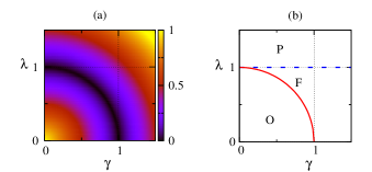
Figure 1: (color online). (a) Energy gap between the ground and first excited states as a function of $\lambda$ and $\gamma$ for two qubits with XY type interaction. The level crossing (dark line) takes places on the circle $\lambda^{2}+\gamma^{2}=1$. (b) The ground state phase diagram of the XY model. P denotes the paramagnetic phase, F the ordered ferromagnetic phase, and O the oscillatory phase Barouch71 .

It is remarkable that the ground state and the ground-state energy of the XY model are similar in forms to Eqs. (7a) and (7b), respectively. One may wonder why the phase diagram of two qubits with XY type interaction looks like that of the XY model in thermodynamic limit, as depicted in Fig. 1. This could be explained by the fact that the ground state energy $E_{0}$ of a system of $N$ identical particles with at most two particle interaction can be written as $E_{0}=\frac{N}{2}\sum_{i}\epsilon_{i}\langle{\epsilon_{i}}|D^{2}|{\epsilon_{i}}\rangle$  Coleman , where $D^{2}={\rm tr}_{3,\dots,N}\left(|{\Psi}\rangle\langle{\Psi}|\right)$ is the two-particle reduced density matrix derived from the ground state $|{\Psi}\rangle$ satisfying $H|{\Psi}\rangle=E_{0}|{\Psi}\rangle$. And the reduced Hamiltonian $K\equiv H_{1}+H_{2}+(N-1)H_{12}$, derived from the full Hamiltonian $H=\sum_{i=1}^{N}H_{i}+\sum_{i<j}H_{ij}$, has eigenvalues $\epsilon_{i}$ and eigenstates $|{\epsilon_{i}}\rangle$. The XY model can be mapped to an one-dimensional spinless fermion system through the Jordan-Wigner transformation. Thus one can see why the eigenvalues and eigenstates of Hamiltonian (1) contain the partial information on the XY model Oh08 .

Now, let us examine whether the entanglement is always a good indicator to quantum phase transitions Osterloh02 ; Osborne02 ; Amico08 . For a pure two-qubit state $|{\psi}\rangle=a|{00}\rangle+b|{01}\rangle+c|{10}\rangle+d|{11}\rangle$ with $|a|^{2}+|b|^{2}+|c|^{2}+|d|^{2}=1$, a well-known entanglement measure is the concurrence $C(|{\psi}\rangle)=2|ad-bc|$. For the ground state $|{\psi_{0}}\rangle$ given by $|{E_{-}^{e}}\rangle$ and $|{E_{-}^{o}}\rangle$, it is written as

$$C(|{\psi_{0}}\rangle)=\begin{cases}\sin\theta&\text{for}\quad\gamma^{2}+\lambda^{2}>1\,,\\ 1&\text{for}\quad\gamma^{2}+\lambda^{2}<1\,.\end{cases}$$ (10)

As shown in Fig. 2 (a), the entanglement changes abruptly as $\gamma$ and $\lambda$ passes across the circle, i.e., the disorder line. It seems that the entanglement works well as an indicator to quantum phase transitions. However, along the $\gamma$ axis, i.e., $\theta=\pi/2$, the concurrence doesn’t change even if the ground state changes from $|{E_{-}^{o}}\rangle$ to $|{E_{-}^{e}}\rangle$. This demonstrates that the entanglement may fail to capture a certain quantum phase transition which happens between the ground states with same degrees of entanglement. As the number of particles increase, the dimension of a sub Hilbert space whose states have the same degree of entanglement also increases. It is not hard to imagine a quantum phase transition which occurs between the ground states with the same degree of entanglement. In this case, the entanglement is not a good indicator to quantum phase transitions.

The fidelity $F$ between two quantum states $|{\psi}\rangle$ and $|{\phi}\rangle$, defined by $F\equiv|\langle\psi|\phi\rangle|^{2}$, is one of the useful measures of distance between two quantum states. It could be a good indicator to quantum phase transitions because the ground states before and after the quantum critical points change abruptly Zanardi07 . It is simple to calculate the fidelity $F=|\langle E_{-}^{o}|\psi_{0}\rangle|^{2}$ between the ground state $|{\psi_{0}(\lambda,\gamma}\rangle$ and the reference state $|{E_{-}^{0}}\rangle$ as a function of $\gamma$ and $\lambda$. As illustrated in Fig.  2 (b), the fidelity jumps on the circle.

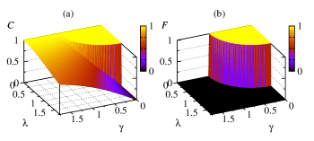
Figure 2: (color online). (a) Concurrence $C(|{\psi_{0}}\rangle)$ of the ground state $|{\psi_{0}}\rangle$ and (b) fidelity $F$ between $|{E_{-}^{0}}\rangle$ and $|{\psi_{0}}\rangle$ as a function of $\gamma$ and $\lambda$.

Let us turn to the relation between geometric phases and quantum phase transitions. The geometric phase has been introduced as an alternative indicator to quantum phase transitions in Refs. Carollo05 ; Zhu06 where the degeneracy points are located on the XX line, i.e., along the $\lambda$ axis, of the XY model. In contrast, the system here has the degeneracy points on the circle. Let us rotate the Hamiltonian about the $\lambda$ axis by angle $\phi$, $\widetilde{H}(\lambda,\gamma,\phi)=U^{{\dagger}}_{z}(\phi)\,H(\lambda,\gamma)\,U_{z}(\phi)$ with $U_{z}(\phi)\equiv\exp\left[-i\frac{\phi}{2}\left(\sigma_{1}^{z}+\sigma_{2}^{z}\right)\right]$. It is easy to obtain the transformed Hamiltonian

$$\widetilde{H}(\lambda,\gamma,\phi)=-\left(\begin{array}[]{cccc}\lambda&0&0&\gamma\,e^{-i2\phi}\\ 0&0&1&0\\ 0&1&0&0\\ \gamma\,e^{i2\phi}&0&0&-\lambda\end{array}\right)\,.$$ (15)

The comparison of Eqs. (6) and (15) shows two things. First, $\widetilde{H}_{\rm odd}$ is independent of angle $\phi$. Second, $\widetilde{H}_{\rm even}$ looks like that of a spin $1/2$ particle in a rotated magnetic field ${\bf B}=\sqrt{\lambda^{2}+\gamma^{2}}\,(\sin\theta\cos 2\phi,\sin\theta\sin 2\phi,\cos\theta)$. Notice that the azimuth angle is $2\phi$ even if the system is rotated by $\phi$. This is due to the bilinear form of Hamiltonian (1). It is instructive to compare it with the rotation of a single spin about $z$-axis by $\phi$, as in a textbook of quantum mechanics Sakurai . The transformed Hamiltonian $\widetilde{H}_{S}$ is given by

$$\widetilde{H}_{S}=R^{\dagger}_{z}\begin{pmatrix}\cos\theta&\sin\theta\\ \sin\theta&-\cos\theta\end{pmatrix}R_{z}=\begin{pmatrix}\cos\theta&\sin\theta\,e^{-i\phi}\\ \sin\theta\,e^{i\phi}&-\cos\theta\end{pmatrix}\,,$$

where $R_{z}=\exp\left[-i\frac{\phi}{2}\sigma_{z}\right]$. This is $2\pi$ periodic in $\theta$ and $\phi$. On the other hand, Hamiltonian (15) is $\pi$ periodic in $\phi$, $\widetilde{H}(\theta,\phi)=\widetilde{H}(\theta+2\pi,\phi+\pi)$.

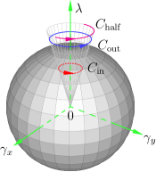
Figure 3: (color online). A monopole sphere is produced by rotating a circle $\gamma^{2}+\lambda^{2}=1$ about $\lambda$ axis by $2\pi$, where the monopole charges corresponding to the degeneracy points are distributed on the surface of the sphere, not located at the origin. Two circuits, $C_{\rm in}$ inside and $C_{\rm out}$ outside the sphere, have the same solid angle. An open path $C_{\rm half}$ outside the sphere is a half rotation, i.e., $\pi$. In spherical coordinates, the radius $r$ is given by $r=\sqrt{\gamma^{2}+\lambda^{2}}$, the polar angle $\theta$ by $\tan\theta=\gamma/\lambda$, and $\gamma=\sqrt{\gamma_{x}^{2}+\gamma_{y}^{2}}$.

Let the ground state of the system be changed adiabatically through the path $C$ in the parameter space ${\bf r}=(r,\theta,\phi)$, as shown in Fig. 3. The instantaneous ground state $|{\psi_{0}({\bf r})}\rangle$ satisfying $\widetilde{H}({\bf r})|{\psi_{0}({\bf r})}\rangle=E_{0}({\bf r})|{\psi_{0}({\bf r})}\rangle$ reads

$$|{\psi_{0}}\rangle=\begin{cases}\cos\tfrac{\theta}{2}e^{-i\phi}\,|{00}\rangle+\sin\tfrac{\theta}{2}e^{i\phi}\,|{11}\rangle&\text{for}\,\,r>1\,,\\[6.0pt] \frac{1}{\sqrt{2}}\left(|{01}\rangle+|{10}\rangle\right)&\text{for}\,\,r<1\,.\end{cases}$$ (16)

For $r>1$, the argument of the exponential function is $\phi$, not $\phi/2$. With Eq. (16), it is easy to calculate the Berry connection or vector potential ${\bf A}_{g}\equiv i\langle{\psi_{0}({\bf r})}|\nabla|{\psi_{0}({\bf r})}\rangle$,

$${\bf A}_{g}=\begin{cases}\displaystyle{-\frac{2}{r\sin\theta}\sin^{2}\frac{\theta}{2}\,\bm{\hat{\phi}}}&\text{for}\quad r>1\,,\\[6.0pt] 0&\text{for}\quad r<1\,.\end{cases}$$ (17)

In Eq. (17), the Berry connection outside the sphere is two times stronger than that of a single $1/2$ spin in a magnetic field. It is evident that the ground state evolving adiabatically inside the sphere acquires no geometric phase,

$$\beta=\oint_{C_{\rm in}}{\bf A}_{g}\cdot d{\bf r}=0\,.$$ (18)

On the other hand, the ground state traveling outside the sphere accumulates the geometric phase

$$\beta=\oint_{C_{\rm out}}{\bf A}_{g}\cdot d{\bf r}=-2\pi(1-\cos\theta)=-\Delta\Omega\,,$$ (19)

where $\Delta\Omega$ is the solid angle bounded by $C_{\rm out}$. One may feel puzzled on why the geometric phase is twice of $\beta=-s\Delta\Omega$ of spin $s=1/2$ even if the quantum state outside the sphere looks like that of a single spin. The reason is that the Hamiltonian $\widetilde{H}(\lambda,\gamma,\phi)$ has the period of $\pi$ in $\phi$. So, the quantum state traveling along the half-circuit $C_{\rm half}$ as shown in Fig. 3 gets $\beta=-\pi(1-\cos\theta)$ but the path in the parameter space is not closed. This is closely related to the fact that a single spin returns to its original state after the $4\pi$ rotation, but the $2\pi$ rotation gives the minus sign Rauch75 ; Sakurai . In our case, consider the action of the operator $U_{z}(\phi)$ on the entangled state $|{\Phi^{(+)}}\rangle=\frac{1}{\sqrt{2}}(|{00}\rangle+|{11}\rangle)$. One obtains $U_{z}^{\dagger}(\phi)|{\Phi^{(+)}}\rangle=\frac{1}{\sqrt{2}}(e^{i\phi}|{00}\rangle+e^{-i\phi}|{11}\rangle)$. Thus the entangled state $|{\Phi^{(+)}}\rangle$ gets back to its original state after the $2\pi$ rotation but not $4\pi$. It is possible to detect the global minus sign change in $|{\Phi^{(+)}}\rangle$ under the $\pi$ rotation. Notice that a product state $\frac{1}{2}(|{0}\rangle_{1}+|{1}\rangle_{1})(|{0}\rangle_{2}+|{1}\rangle_{2})$ doesn’t get the global minus sign under the $\pi$ rotation of $U_{z}(\phi)$. The magnetic monopole field ${\bf B}_{g}=\nabla\times{\bf A}_{g}$ is written as

$${\bf B}_{g}=\left\{\begin{array}[]{cc}-\displaystyle{\frac{2}{r^{2}}\,{\bm{\hat{}}{\bf r}}}&\text{for}\quad r>1\,,\\[6.0pt] 0&\text{for}\quad r<1\,.\end{array}\right.$$ (22)

This is completely analogous to the electric field produced by a conducting sphere with charge $q=-2$.

Let us take a look at when the geometric phase fails to capture the quantum phase transition. Consider the level crossing along the line $\gamma=1$ as shown in Fig. 4. The ground state energy $E_{-}^{e}(\lambda,1)=-\sqrt{1+\lambda^{2}}$ meets the first exited energy $E_{-}^{o}(\lambda,1)=-1$ at $\lambda=0$, but they don’t cross each other. This is known as the Renner-Teller or glancing intersection, which differs from the conical intersection in the sense that the Renner-Teller intersection points is not a source of geometric phase Zwanziger87 . To this end, let us rotate the Hamiltonian $H(\lambda,1)=-\sigma_{1}^{x}\sigma_{2}^{x}-\frac{\lambda}{2}\left(\sigma_{1}^{z}+\sigma_{2}^{z}\right)$ with $U_{x}(\phi)\equiv\exp\left[-i\frac{\phi}{2}(\sigma^{x}_{1}+\sigma^{x}_{2})\right]$. It is easy to show that two energy levels $E_{-}^{e}(\lambda,1)$ and $E_{-}^{o}(\lambda,1)$ have the cylindrical symmetry, i.e., independent of $\phi$, as depicted in Fig. 4. The ground state of the transformed Hamiltonian $\widetilde{H}(\lambda,\phi)=U_{x}^{{\dagger}}(\phi)H(\lambda,1)U_{x}(\phi)$ is given by $|{\psi_{0}(\phi)}\rangle=(a\,\cos^{2}\frac{\phi}{2}-b\,\sin^{2}\frac{\phi}{2})\,|{00}\rangle+i\frac{a+b}{2}\sin\phi\,|{01}\rangle+i\frac{a+b}{2}\sin\phi\,|{10}\rangle+(b\,\cos^{2}\frac{\phi}{2}-a\,\sin^{2}\frac{\phi}{2})\,|{11}\rangle$, where $a=\cos\frac{\theta}{2},b=\sin\frac{\theta}{2}$, and $\tan\theta=1/\lambda$. Clearly there is no sign change in $|{\psi_{0}(\phi)}\rangle$ under the rotation of $\phi$ by $2\pi$.

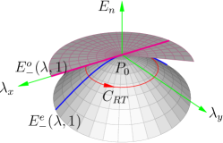
Figure 4: (color online). Renner-Teller intersection at the point of $\gamma=1$ and $\lambda=0$.

Let us discuss an experimental aspect of the main results presented here. Since the system considered here is composed of only two qubits, it may not be hard to verify them with NMR qubits Jones00 ; Zhang08 , ion-trap qubits Leibfried03 , superconducting qubits Leek07 . With these systems, the geometric phase of a single qubit has been already reported.

In conclusion, we have studied the system of two qubits with XY type interaction to investigate whether the entanglement, the fidelity, and the geometric phases are good indicators to quantum phase transitions. First, it has been shown that the phase diagram of two qubits with XY type interaction is same to the disorder line in the XY model. Second, we have presented the counter examples that the entanglement and the geometric phase fail to detect a certain quantum phase transition. As shown before, there is a quantum phase transition between the ground states with same degrees of entanglement. A quantum state traveling around the quantum phase transition point of the Renner-Teller intersection acquires no geometric phase. Finally, we have found the magnetic monopole sphere, only outside which the quantum state acquires the geometric phase, in perfect analogy to a charged conducting sphere.

- (1) A. Zener, Proc. Roy. Soc. A 137, 696 (1932).
- (2) E. Farhi et al., Science 292, 472 (2001).
- (3) M.V. Berry, Proc. R. Soc. London Ser. A 392, 45 (1984).
- (4) A. Shapere and F. Wilczek, Geometric phases in physics, (World Scientific, Singapore, 1989).
- (5) S. Sachdev, Quantum phase transitions, (Cambridge Univ. Press, Cambridge, 1999).
- (6) M. Vojta, Rep. Prog. Phys. 66, 2069 (2003).
- (7) A. Osterloh, L. Amico, G. Falci, and R. Fazio, Nature (London) 416, 608 (2002).
- (8) T.J. Osborne and M.A. Nielsen, Phys. Rev. A66, 032110 (2002).
- (9) L. Amico, R. Fazio, A. Osterloh, and V. Vedral, Rev. Mod. Phys. 80, 517 (2008).
- (10) A.C.M. Carollo and J.K. Pachos, Phys. Rev. Lett. 95, 157203 (2005).
- (11) S.-L. Zhu, Phys. Rev. Lett. 96, 077206 (2006).
- (12) P. Zanardi, P Giorda, and M. Cozzini, Phys. Rev. Lett. 99, 100603 (2007); M. Cozzini, P. Giorda, and P. Zanardi, Phys. Rev. B75, 014439 (2007).
- (13) E. Lieb , T. Schultz, and D. Mattis. Ann. of Phys. (N.Y.) 16, 407 (1961); S. Katsura, Phys. Rev. 127, 1508 (1962).
- (14) E. Barouch and B.M. McCoy, Phys. Rev. A3, 786 (1971); M. Suzuki, Prog. Theor. Phys. 46, 1337 (1971).
- (15) A.J. Coleman and V.I. Yukalov, Reduced Density Matrices, (Springer-Verlag, Berlin, 2000).
- (16) S. Oh, in preparation.
- (17) J.J. Sakurai, Modern Quantum Mechanics, (The Benjamin/Cummings, California, 1985).
- (18) H. Rauch et al., Phys. Lett. A 54, 425 (1975); S.A. Werner et al., Phys. Rev. Lett. 35, 1053 (1975).
- (19) J.W. Zwanziger and E.R. Grant, J. Chem. Phys. 87, 2954 (1987).
- (20) J. Zhang, X. Peng, N. Rajendran, and D. Suter, Phys. Rev. Lett. 100, 100501 (2008).
- (21) J.A. Jones, V. Vedral, A. Ekert, and G. Gastagnoli, Nature 403, 869 (2000).
- (22) D. Leibfried et al., Nature 422, 412 (2003).
- (23) P.J. Leek et al., Science 318, 1889 (2007).