INSTITUT NATIONAL DE RECHERCHE EN INFORMATIQUE ET EN AUTOMATIQUE

Energy-delay bounds analysis in wireless multi-hop networks with unreliable radio links
Ruifeng Zhang — Jean-Marie Gorce — Katia Jaffrès-Runser N° 6598
July, 25, 2008

Abstract: Energy efficiency and transmission delay are very important parameters for wireless multi-hop networks. Previous works that study energy efficiency and delay are based on the assumption of reliable links. However, the unreliability of the channel is inevitable in wireless multi-hop networks. This paper investigates the trade-off between the energy consumption and the end-to-end delay of multi-hop communications in a wireless network using an unreliable link model. It provides a closed form expression of the lower bound on the energy-delay trade-off for different channel models (AWGN, Raleigh flat fading and Nakagami block-fading) in a linear network. These analytical results are also verified in 2-dimensional Poisson networks using simulations. The main contribution of this work is the use of a probabilistic link model to define the energy efficiency of the system and capture the energy-delay trade-offs. Hence, it provides a more realistic lower bound on both the energy efficiency and the energy-delay trade-off since it does not restrict the study to the set of perfect links as proposed in earlier works.

Key-words: wireless sensor networks, multi-hop networks, energy-delay trade-off, unreliable links, realistic radio channel, fading channel

Analyse du compromis énergie-délai dans les réseaux radio multi-sauts avec liens radio réalistes

Résumé : L’efficacité énergétique et le délai de transmission de bout en bout sont des paramètres très importants pour les réseaux sans fil multi-sauts. Plusieurs études ont été réalisées, sous l’hypothèse de liens radio parfaits (on/off). Pourtant, en environnement réel, les liens radio sont par essence erratiques, et les erreurs de transmission ne peuvent tre omises. Dans ce rapport, nous étudions le compromis entre énergie et délai de transmission de bout en bout, pour des communications multi-sauts. Nous dérivons sous forme analytique, une borne inférieure du compromis énergie-délai pour différents modèles de canaux réalistes (AWGN, Rayleigh, Nakagami), et prenant en compte les processus de retransmission pour garantir l’acheminement des paquets. Cette borne calculée pour un réseau linéaire, constitue également une borne inférieure pour les réseaux 2D aléatoires. On montre expérimentalement que cette borne est presque atteinte, si la densité de noeuds est suffisante. La principale contribution de ce travail est l’établissement d’une borne inférieure pour le compromis énergie-délai, sur canal réaliste et sous contrainte de transmission parfaite de bout en bout.

Mots-clés : réseaux de capteurs sans fil, réseaux multi-sauts, compromis énergie-délai, canal radio réaliste, canal á évanouissement

1 Introduction

Energy is a scarce resource for nodes in multi-hop networks such as Wireless Sensor Networks (WSNs) and Ad-Hoc networks [1]. Therefore, energy efficiency is of paramount importance in most of their applications.

Regarding energy efficiency, there are numerous original works addressing the problem at the routing layer, MAC layer, physical layer or from a cross-layer point of view, e.g. [2, 3, 4, 5, 6]. Routing strategies in multi-hop environments have a major impact on the energy consumption of networks. Long-hop routes demand substantial transmission power but minimize the energy cost for reception, computation and etc. On the opposite, routes made of shorter hops use fewer transmission power but maximize the energy cost for reception since there is an increase in the number of hops. M. Haenggi points out several advantages of using long-hop routing in his articles, e.g. [7, 2], among which high energy efficiency is one of the most important factors. These works reveal the importance of the transmission range and its impact on the energy conservation but don’t provide a theoretical analysis on the optimal hop length regarding various networking scenarios. In [3], P. Chen et al. define the optimal one-hop length for multi-hop communications that minimizes the total energy consumption. They also analyze the influence of channel parameters on this optimal transmission range. The same issue is studied in [4] with a Bit-Meter-per-Joule metric where the authors study the effects of the network topology, the node density and the transceiver characteristics on the overall energy expenditure. This work is improved by J. Deng et al. in [5].

Since the data transmitted is often of a timely nature, the end-to-end transmission delay becomes a an important performance metric. Hence, minimum energy paths and the trade-off between energy and delay have been widely studied, e.g. [6, 8, 9]. However, unreliable links are not considered in the aforementioned works. In fact, experiments in different environments and theoretical analyzes in [10, 11, 12, 13, 14] have proved that unreliable links have a strong impact on the performance of upper layers such as MAC and routing layer. In our previous work [14], we have shown how unreliable link improve the connectivity of WSNs.

In [15], S. Banerjee et al. take unreliable links into account in their energy efficiency analysis by introducing a link probability and the effect of link error rate. The authors derive the minimum energy paths for a given pair of source and destination nodes and propose the corresponding routing algorithm. However, the energy model used in this paper includes the transmission power only and does not consider circuitry energy consumption at the transmitter and receiver side. In fact, such a model leads to an unrealistic conclusion which states that the smaller hop distance, the higher energy efficiency. As we show in this paper, considering a constant circuitry power according to [16] results in completely different conclusions. Furthermore, we propose to evaluate the effect of fading channel on the energy efficiency.

In this work, we do not consider any specific protocol and assume the corresponding overhead to be negligible. Depending on the application, the energy efficiency has a different significance [16]. A periodic monitoring application is assumed here where the energy spent per correctly received bit is a crucial energy metric. Moreover, in wireless communications, the energy cost augments with the increase of the transmission distance. Hence, we also adopt the mean Energy Distance Ratio per bit ($\overline{EDRb}$) metric in $J/m/bit$ proposed in [4]. A realistic unreliable link model [14] is introduced into the energy model. The purpose of this work is to provide a lower bound on the energy efficiency of both single and multi-hop transmissions and derive the corresponding average transmission delay. As such, we are able to show the theoretical trade-off between the energy efficiency and the delay for single-hop and multi-hop transmissions. The multi-hop case is analyzed in a homogeneous linear network. Both studies are performed over three different channels (i.e. AWGN, Rayleigh flat fading and Nakagami block fading channel). Theoretical results are then validated in 2-dimensional Poisson distributed network using simulations.

The contributions of this paper are:

• The close-form expressions for the optimal transmission range and for the corresponding optimal transmission power are derived in AWGN channel, Rayleigh flat fading channel and Nakagami block fading channel employing both a comprehensive energy model and an unreliable link model.

• The definition of a closed form expression for the lower bound of energy efficiency of a multi-hop communication is obtained in a linear network over three types of channel and is validated by simulation in 2-dimensional Poisson networks.

• The definition of a lower bound for the energy-delay trade-off for a linear and a Poisson network in the three types of channel aforementioned.

This paper is organized as follows: Section 2 concentrates on presenting the models and metrics used in the paper. Section 3 derives a closed form expression of optimal transmission range and optimal transmission power for one-hop transmission. In section 4, the minimum energy reliable path for linear networks and its delay are deduced. In section 5, we focus on the optimal trade-off between the energy consumption and the delay in linear networks. Simulations are given and analyzed in section 6 for a 2-dimensional network. Finally, section 7 concludes our work.

2 Models and Metric

In this section, the energy model, the realistic unreliable link model, the delay model and the metric $\overline{EDRb}$ used in this work are introduced.

2.1 Energy consumption model

We consider energy efficient nodes, i.e. nodes that only listen to the transmissions intended to themselves and that send an acknowledgment packet (ACK) to the source node after a correct packet reception. As such, the energy consumption for transmission of one packet $E_{p}$ is composed of three parts: the energy consumed by the transmitter $E_{Tx}$, by the receiver $E_{Rx}$ and by the acknowledgement packet exchange $E_{ACK}$:

$$E_{p}=E_{Tx}+E_{Rx}+E_{ACK}$$ (1)

The transmission energy model [16] is given by:

$$E_{Tx}=T_{start}\cdot P_{start}+\frac{N_{b}}{R}\cdot(P_{txElec}+\alpha_{amp}+\beta_{amp}\cdot P_{t})$$ (2)

where $P_{t}$ is transmission power, the other parameters are described in Table 1 and $P_{txElec}$ is considered as constant.

Table 1: Some parameters of the transceiver energy consumption[16]

Symbol	Description	Value
$P_{start}$	Startup power	$58.7~{}mW$
$T_{start}$	Startup time	$446~{}\mu s$
$P_{txElec}$	Transmitter circuitry power	$151~{}mW$
$\alpha_{amp}$	Amplifier constant power	$174~{}mW$
$\beta_{amp}$	Amplifier proportional offset ($>1$)	$5.0$
$P_{rxElec}$	Receiver circuitry power	$279~{}mW$
$N_{b}$	Number of bits per packet	$2560$
$R$	Transmission bit rate	$1~{}Mbps$
$N_{0}$	Noise level	$-154dBm/Hz$
$f_{c}$	Carrier frequency	$2.4GHz$
$G_{Tant}$	Transmitter antenna gain	$1$
$G_{Rant}$	Receiver antenna gain	$1$
$\alpha$	Path-loss exponent	$3$
$L$		$1$
$T_{ACK}$	ACK Duration	$5mS$

Similarly, the energy model on the receiver side includes two parts: the startup energy consumption, which is considered identical to the one of the transmitter, and the circuitry cost [16]:

$$E_{Rx}=T_{start}\cdot P_{start}+\frac{N_{b}}{R}\cdot P_{rxElec}.$$ (3)

where $P_{rxElec}$ is the circuity power of the receiver which is considered as constant.

In the acknowledgment process, it is assumed that the ACK packet can be successfully transmitted in a single attempt which is based on the following facts: firstly, since ACK packets are much smaller data packets, their link probability is greater than that of data packet. For instance, for respectively ACK and Data packets of 80 and 320 bytes each, if the successful transmission probability of the data packet is $80\%$, the link probability for the ACK packet is $95\%$. Secondly, assuming a symmetric channel, if the data packet experienced a good channel, the return path experiences the same beneficial channel conditions. Hence, we can assume that only one ACK packet is sent with high probability of success to the source of the message.

Since the energy consumed by the transmission power $P_{t}$ for the ACK packet has small proportion in its total energy, $P_{t}$ is neglected in the energy expenditure model given by:

$$E_{ACK}=(P_{txElec}+P_{rxElec}+\alpha_{amp})\cdot T_{ACK},$$ (4)

where $T_{ACK}$ is the average time during which the transmitter waits for an ACK packet.

The analysis of $E_{p}$ shows that the energy consumption can be classified into two parts: the first part is constant, including $T_{start}\cdot P_{start}$, $P_{txElec}$, $~{}\alpha_{amp}$, $P_{rxElec}$ and $E_{ACK}$, which are independent of the transmission range; the second part is variable and depends on the transmission energy $P_{t}$ which is tightly related to the transmission range. Accordingly, the energy model for each bit follows:

$$E_{b}=\frac{E_{p}}{N_{b}}=E_{c}+K_{1}\cdot P_{t},$$ (5)

where $E_{b}$, $E_{c}$ and $K_{1}\cdot P_{t}$ are respectively the total, the constant and the variable energy consumption per bit. Substituting (1) (2) (3) (4) into (5) yields:

$$E_{c}= \frac{2T_{start}\cdot P_{start}}{N_{b}}+$$

$$(P_{txElec}+P_{rxElec}+\alpha_{amp})(\frac{1}{R}+\frac{T_{ACK}}{N_{b}})$$ (6)

$$K_{1}= \frac{\beta_{amp}}{R}.$$ (7)

For a given transmitting/receiving technology, $E_{c}$ and $K_{1}$ are constant because all parameters in (6) and (7) are fixed. Then $E_{b}$ becomes a function of $P_{t}$, i.e., $E_{b}(P_{t})$.

2.2 Realistic unreliable link model

The unreliable radio link model is defined using the packet error rate (PER) [14]:

$$p_{l}(\gamma_{x,x^{\prime}})=1-PER(\gamma_{x,x^{\prime}})$$ (8)

where $PER(\gamma)$ is the PER obtained for a signal to noise ratio (SNR) of $\gamma$. The PER depends on the transmission chain technology (modulation, coding, diversity … ). And $\gamma_{x,x^{\prime}}$ is calculated by [16]:

$$\gamma_{x,x^{\prime}}=K_{2}\cdot P_{t}\cdot d_{x,x^{\prime}}^{-\alpha},$$ (9)

with

$$K_{2}=\frac{G_{Tant}\cdot G_{Rant}\cdot\lambda^{2}}{(4\pi)^{2}N_{0}\cdot B\cdot L},$$ (10)

where $d_{x,x^{\prime}}$ is the transmission distance between node $x$ and $x^{\prime}$, $\alpha\geq 2$ is the path loss exponent, $P_{t}$ is the transmission power, $G_{Tant}$ and $G_{Rant}$ are the antenna gains for the transmitter and receiver respectively, $B$ is the bandwidth of the channel and is set to $B=R$, $\lambda$ is the wavelength and $L\geq 1$ summarizes losses through the transmitter and receiver circuitry.

Similar to $E_{b}$, for a given technology, $K_{2}$ becomes a constant. And $p_{l}(\gamma(x,x^{\prime}))$ can be rewritten as a function of $d$ and $P_{t}$, i.e., $p_{l}(d,P_{t})$.

2.3 Mean energy distance ratio per bit ($\overline{EDRb}$)

The mean Energy Distance Ratio per bit ($\overline{EDRb}$) [4] in $J/bit/m$ is defined as the energy consumption for transmitting one bit over one meter. The mean energy consumption per bit for the successful transmission over one hop $\overline{E}_{1hop}$ including the energy needed for retransmissions is given by:

$$\overline{E}_{1hop} =E_{b}(P_{t})\cdot\sum_{n=1}^{\infty}n\cdot p_{l}(d,P_{t})\cdot(1-p_{l}(d,P_{t}))^{(n-1)}$$

$$=E_{b}(P_{t})\cdot\frac{1}{p_{l}(d,P_{t})}$$ (11)

where $n$ is the number of retransmissions. According to its definition, $\overline{EDRb}$ is given by:

$$\overline{EDRb}=\frac{\overline{E}_{1hop}}{d}=\frac{E_{b}(P_{t})}{d\cdot p_{l}(d,P_{t})}=\frac{E_{c}+K_{1}\cdot P_{t}}{d\cdot p_{l}(d,P_{t})}.$$ (12)

2.4 Delay model

The average delay for a packet to be transmitted over one hop, $D_{onehop}$, is defined as the sum of three delay components. The first component is the queuing delay during which a packet waits for being transmitted. The second component is the transmission delay that is equal to $N_{b}/R$. The third component is $T_{ACK}$. Note that we neglect the propagation delay because the transmission distance between two nodes is usually short in multi-hop networks. Without loss of generality, $D_{onehop}$ is set to be $1$ unit. However, one-hop transmission may suffer from the delay caused by retransmissions. According to (2.3), the mean delay of a reliable one-hop transmission is:

$$\overline{D} =D_{onehop}\times mean\ number\ of\ retransmissions$$

$$=\frac{1}{p_{l}(d,P_{t})}.$$ (13)

3 One-hop Transmission: Energy Efficiency and Delay

The one-hop transmission is the building block of a multi-hop path. In this section, we derive the optimal transmission range and power that minimizes the energy expenditure of the one-hop transmission by introducing three different channel models. Optimal transmission range $d_{0}$ and optimal transmission power $P_{0}$ are calculated according to:

$$\frac{\partial{\overline{EDRb}}}{\partial{P_{t}}}=\frac{\partial}{\partial{P_{t}}}\left(\frac{E_{b}(P_{t})}{d\cdot p_{l}(d,P_{t})}\right)\Bigg{|}_{P_{t}=P_{0}} =0$$ (14)

$$\frac{\partial{\overline{EDRb}}}{\partial{d}}=\frac{\partial}{\partial d}\left(\frac{E_{b}(P_{t})}{d\cdot p_{l}(d,P_{t})}\right)\Bigg{|}_{d=d_{0}} =0.$$ (15)

The optimal transmission power $P_{0}$ and range $d_{0}$ exist because for smaller values of $d$, the transmission power $P_{t}$ is low in terms of a certain link probability and the constant energy component $E_{c}$ is dominating in $\overline{EDRb}$ consequently; for higher values of $d$, the variable energy consumption $K_{1}\cdot P_{t}$ is dominating $\overline{EDRb}$ since $P_{t}$ increases proportionally to $d^{\alpha}$ in order to reach the destination.

3.1 Energy-optimal transmission power $P_{0}$

Substituting (8) into (14) and (15) and simplifying, according to the derivation in Appendix A, we obtain:

$$P_{0}=\frac{E_{c}}{K_{1}(\alpha-1)}.$$ (16)

Substituting (6) and (7) into (16) yields:

$$P_{0}= \frac{1}{\alpha-1}\left(\frac{2T_{start}\cdot P_{start}}{\frac{N_{b}}{R}\beta_{amp}}\right)$$

$$+\left(\frac{1}{\beta_{amp}}+\frac{T_{ACK}}{\frac{N_{b}}{R}\beta_{amp}}\right)\frac{P_{txElec}+P_{rx}+\alpha_{amp}}{\alpha-1},$$ (17)

where $N_{b}/R$ is the transmission duration.

In (3.1), it should be noted that $P_{0}$ is independent from $p_{l}(\gamma)$ and consequently independent from modulation and fading. In general, $N_{b}/R\gg T_{start}$. Following, the first part of (3.1) can be neglected. On the opposite, the characteristics of the amplifier have a strong impact on $P_{0}$. When the efficiency of the amplifier is high, i.e. $\beta_{amp}\rightarrow 1$, $P_{0}$ reaches its maximum value resulting in a longer optimal transmission range $d_{0}$. It tallies with the result of [17]. It is clear that when the environment of transmission deteriorates, namely, $\alpha$ increases, $P_{0}$ decreases correspondingly.

3.2 Energy-optimal transmission range $d_{0}$ and its delay

According to Appendix A, $d_{0}$ follows:

$$d_{0}^{\alpha}=\frac{p_{l}^{\prime}(\gamma)K_{2}P_{0}}{p_{l}(\gamma)},~{}{\rm with~{}}\gamma=K_{2}P_{0}d_{0}^{-\alpha}$$ (18)

where $p_{l}^{\prime}(\gamma)$ is the first derivative of $p_{l}(\gamma)$. Equation (18) indicates that $d_{0}$ depends on $p_{l}(\gamma)$ and hence has to be analyzed according to the type of channel and modulation as proposed next. This expression is meaningful since it can be used to estimate the optimal node density in a wireless netework depending on $pl(\gamma)$.

3.2.1 AWGN channel

The optimal transmission range in AWGN channel, which is derived in Appendix B, is obtained by:

$$d_{0g}=\left(\frac{-0.5415\beta_{m}K_{2}N_{b}E_{c}\alpha}{K_{1}(\alpha-1)(1+\alpha N_{b}\text{W}_{-1}\left[\frac{-e^{-\frac{1}{N_{b}\cdot\alpha}}}{0.1826\alpha_{m}N_{b}\alpha}\right])}\right)^{\frac{1}{\alpha}}$$ (19)

where $\text{W}_{-1}[\cdot]$ is the branch satisfying $\text{W}(x)<-1$ of the Lambert W function [18].

Substituting (16) and (19) into (9), the optimal SNR $\gamma_{0g}$ is given by:

$$\gamma_{0g}=\frac{1+\alpha N_{b}\text{W}_{-1}\left[-\frac{e^{-\frac{1}{N_{b}\cdot\alpha}}}{0.1826\alpha_{m}N_{b}\alpha}\right]}{-0.5415\beta_{m}kN_{b}\alpha}.$$ (20)

Meanwhile, the optimal BER is obtained by (20) and (48):

$$BER_{0g}=0.1826\alpha_{m}\exp(\frac{1+\alpha N_{b}\text{W}_{-1}\left[\frac{-e^{-\frac{1}{N_{b}\cdot\alpha}}}{0.1826\alpha_{m}N_{b}\alpha}\right]}{N_{b}\alpha}).$$ (21)

Depending on $\gamma_{0g}$ and $BER_{0g}$, the receiver can decide whether it is in the optimal communication range or not by measuring its channel state.

The delay and the energy efficiency of the one-hop communication can be analyzed by expressing respectively the delay $D_{g}$ and the energy metric $\overline{EDRb}$ as a function of the transmission range $d$ as detailed in Appendix B. Hence, substituting (48) into (2.4), the delay of the reliable one-hop transmission in AWGN channel as a function of $d$ is given by:

$$\overline{D}_{g}=\left(1-0.1826\alpha_{m}\cdot\exp(-0.5415\beta_{m}K_{2}P_{t}d^{-\alpha})\right)^{-N_{b}}.$$ (22)

Substituting (46) into (14), the optimal transmission power $P_{0g}$ as a function of the transmission distance $d$ achieving energy efficiency in AWGN channel follows:

$$P_{0g}(d)=\frac{d^{\alpha}+N_{b}d^{\alpha}\text{W}_{-1}\left[\frac{\exp\left(-\frac{0.5415E_{c}K_{2}\beta_{m}}{K_{1}d^{\alpha}}-\frac{1}{N_{b}}\right)}{-0.1826\alpha_{m}N_{b}}\right]}{-0.5415\beta_{m}K_{2}N_{b}}-\frac{E_{c}}{K_{1}}.$$ (23)

Substituting (23) and (48) into (12), $\overline{EDRb}$ as a function of $d$ in AWGN channel is expressed by:

$$\overline{EDRb}(d)=\frac{E_{c}+K_{1}P_{0g}(d)}{d\left(1-BER_{g}(K_{2}P_{0g}(d)d^{-\alpha})\right)^{N_{b}}}.$$ (24)

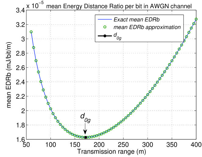
Figure 1: $\overline{EDRb}$ of the one-hop transmission as a function of the range $d$ in AWGN channel where $d_{0g}=172.31m$, $P0=180.51mW$, $\gamma_{0g}=9.34dB$, $BER_{0g}=1.37e-5$, $p_{l}=96.55\%$ and $\overline{D}_{g}=1.04$ unit. The exact $\overline{EDRb}$ is obtained with (47) and the approximation of $\overline{EDRb}$ is obtained with (48). Therefore, the approximation is feasible. .

Fig. 1 shows the variation of $\overline{EDRb}$ with the transmission range $d$ in AWGN channel as an example according to (24), where BPSK modulation is adopted. The related parameters are listed in Table 1. It should be noted that the value of $p_{l}$ is close to $1$, which shows that energy optimal links in AWGN channel are reliable.

3.2.2 Rayleigh flat fading channel [19]

The optimal transmission range $d_{0f}$ in Rayleigh flat fading channel, which is derived in Appendix C, is obtained by:

$$d_{0f}=\left(\frac{2\beta_{m}E_{c}\cdot{K_{2}}}{(\alpha-1)\cdot{K_{1}}\alpha_{m}(\alpha N_{b}+1)}\right)^{\frac{1}{\alpha}}.$$ (25)

The expression of $d_{0f}$ shows that it decreases with the increase of $\alpha$ or $N_{b}$.

Substituting (16) and (25) into (9) provides the optimal SNR in Rayleigh flat fading channel:

$$\bar{\gamma}_{0f}=(\alpha N_{b}+1)\frac{\alpha_{m}}{2\beta_{m}}\approx\frac{\alpha N_{b}\cdot\alpha_{m}}{2\beta_{m}}~{}~{}(\alpha N_{b}\gg 1).$$ (26)

Then substituting  (26) into (50), the optimal BER in Rayleigh flat fading channel is:

$$BER_{0f}=\frac{1}{\alpha N_{b}+1}\approx\frac{1}{\alpha N_{b}}.$$ (27)

From a cross layer point of view, the routing layer can identify if a node is at the optimal communication range according to the values of $\bar{\gamma}_{0f}$ or $BER_{0f}$.

Similarly to the study in AWGN channel, we derive here the expression of the delay $D_{f}$ and the energy metric $\overline{EDRb}$ as a function of the transmission range $d$ which is detailed in Appendix C. Substituting (50) into (2.4), the delay of the reliable one-hop transmission in a Rayleigh flat fading channel as a function of $d$ is given by:

$$\overline{D}_{f}=\left(1-\frac{\alpha_{m}}{2\beta_{m}K_{2}P_{t}d^{-\alpha}}\right)^{-N_{b}}.$$ (28)

Substituting (51) into (14), the optimal transmission power $P_{0f}$ as a function of the transmission distance $d$ achieving energy efficiency in a Rayleigh channel follows:

$$P_{0f}(d)= \frac{d^{a}(1+N_{b})\alpha_{m}}{4K_{2}\beta_{m}}+\frac{\sqrt{d^{\alpha}K_{1}\alpha_{m}(d^{\alpha}K_{1}(1+N_{b})^{2}\alpha_{m}+8E_{c}K_{2}N_{b}\beta_{m})}}{4K_{2}K_{1}\beta_{m}}$$ (29)

Hence, for a given transmission distance, the optimal transmission power can be derived according to $P_{0f}(d)$ in an adaptive power configuration.

Finally, $\overline{EDRb}$ as a function of $d$ is computed by substituting  (29) into (12):

$$\overline{EDRb}(d)=\frac{E_{c}+K_{1}P_{0f}(d)}{d\left(1-\frac{\alpha_{m}}{2\beta_{m}K_{2}\cdot P_{0f}(d)\cdot d^{-\alpha}}\right)^{N_{b}}}$$ (30)

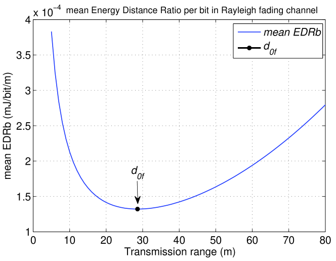
Figure 2: $\overline{EDRb}$ of the one-hop transmission as a function of the range $d$ in Rayleigh flat fading channel where $P_{0}=180.51mW$, $d_{0f}=15.97m$, $\gamma_{0f}=32.83dB$, $BER_{0f}=1.30e-4$, $p_{l}=0.72$ and $\overline{D}_{f}=1.40$.

Fig. 2 shows that $\overline{EDRb}$ varies with $d$ according to (30) in a Rayleigh flat fading channel. The parameters related are listed in table 1. Having $p_{l}=0.7165$ shows that an energy optimal link in Rayleigh channel is far less reliable than the link in AWGN channel. This result claims for using unreliable links in the real deployment of wireless network.

3.2.3 Nakagami block fading channel

The link model in Nakagami block fading channel, as shown in (53), is too complex to obtain the closed form expression of the energy optimal transmission distance $d_{0b}$. Therefore, two scenarios are taken into consideration in the following.

Firstly, when $m=1$ and $\alpha_{m}=1$ (e.g., for BPSK, BFSK and QPSK), according to the derivation in Appendix D, the optimal transmission range $d_{0b}$ in Nakagami block fading channel is:

$$d_{0b}=\left(\frac{\beta_{m}K_{2}E_{c}}{K_{1}(\alpha^{2}-\alpha)(4.25\log_{10}(N_{b})-2.2)}\right)^{1/\alpha}.$$ (31)

Substituting (16) and (31) into (9) yields the optimal signal to noise ratio in Nakagami block fading channel:

$$\overline{\gamma}_{0b}=\frac{\alpha}{\beta_{m}}(4.25\log_{10}(N_{b})-2.2)$$ (32)

For a given transmission range, we can obtain the optimal transmission power $P_{0b}$ in Nakagami block fading channel using  (14) and (55):

$$P_{0b}(d)=\frac{-2E_{c}}{K_{1}-\frac{\sqrt{K_{1}(4E_{c}\beta_{m}K_{2}-2.2d^{\alpha}K_{1}+4.25d^{\alpha}K_{1}\log_{10}(N_{b}))}}{\sqrt{d^{\alpha}(4.25\log_{10}(N_{b})-2.2)}}}.$$ (33)

Finally, $\overline{EDRb}$ as a function of $d$ is obtained by substituting (33) into (12):

$$\overline{EDRb}(d)=\frac{E_{c}+K_{1}P_{0b}(d)}{d\exp\left(\frac{-4.25\log_{10}(Nb)+2.2}{\beta_{m}K_{2}P_{0b}(d)d^{-\alpha}}\right)^{N_{b}}}.$$ (34)

Substituting (53) into (2.4), we get the delay of a reliable one-hop $\overline{D}_{b}$ in Nakagami block fading channel:

$$\overline{D}_{b}=\frac{1}{\int_{\gamma=0}^{\infty}(1-BER(\gamma))^{N_{b}}p(\gamma|K_{2}P_{t}d^{-\alpha})d\gamma}.$$ (35)

For the other scenarios, the sequential quadratic programming (SQP) method algorithm in [20] is adopted to solve the optimization problem related to the computation of the optimal $\overline{EDRb}$.

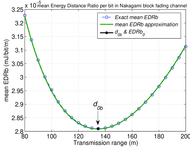
Figure 3: $\overline{EDRb}$ of the one-hop transmission as a function of the range $d$ in Nakagami-m block fading channel where $m=1$, $\alpha_{m}=1$, $P_{0}=180.50mW$, $d_{0b}=134.16m$, $\gamma_{0b}=12.69dB$, $BER_{0b}=6.67e-005$, $p_{l}=0.72$ and $\overline{D}_{b}=1.40$. The exact $\overline{EDRb}$ is obtained with (53) and the approximation of $\overline{EDRb}$ is obtained with (55). Therefore, this is an suitable approximation.

Fig. 3 shows how $\overline{EDRb}$ varies with $d$ according to Eq. (34) in Nakagami block fading channel using BPSK modulation. The related parameters are presented in table 1. Having $p_{l}=0.72$ reveals that energy optimal links in Nakagami block fading channel are even more unreliable than those in Rayleigh flat fading channel.

From Fig. 1, Fig. 2 and Fig. 3, it can be concluded that: firstly, the optimal transmission power $P_{0}$ corresponding to the optimal transmission range is the same for all channels which concises with the result of Eq.(16); secondly, the optimal transmission range decreases when fading becomes stronger, namely, from AWGN, Nakagami block fading channel to Rayleigh flat fading channel; thirdly, $\overline{EDRb}$ increases with the enlargement of fading , i.e., more energy has to be consumed to counteract the effect of fading.

3.3 Impact of some physical parameters

This section studies the impact of some physical parameters such as the path-loss exponent $\alpha$, the strength of fading, the circuitry power, $N_{b}$, the transmission rate $R$ and the modulation technique. For all the results provided hereafter, the values of physical parameters that are not analyzed are given in Table 1.

Impact of fading

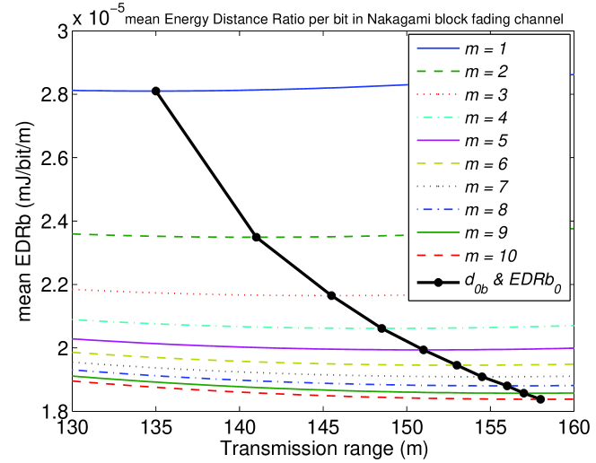
Figure 4: Impact of the strength of fading ($m$) in Nakagami block fading channel for the one-hop transmission energy performance given by $\overline{EDRb}$ as a function of $d$.

The sequential quadratic programming (SQP) algorithm described in [20] is implemented to analyze the impact of strength of fading on the optimal $\overline{EDRb}$ and corresponding optimal transmission range in Nakagami block fading channel. The results are shown in Fig. 4. Similarly to our previous analysis, the increase of the strength of fading leads to the increase of the optimal $\overline{EDRb}$ and shortens the optimal transmission range. In that case, more energy is consumed to overcome the destructive effect of fading.

Impact of the path loss exponent

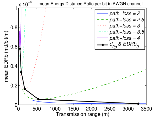
(a) AWGN channel

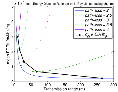
(b) Rayleigh flat fading channel

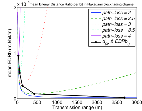
(c) Nakagami block fading channel $m=1$

Figure 5: Impact of the path loss exponent $\alpha$ on the one-hop transmission energy performance given by $\overline{EDRb}$ as a function of $d$.

Fig. 5 shows that $\overline{EDRb}$ greatly increases with the strength of the path loss, i.e., more energy is consumed to make up for the path loss. Meanwhile, path loss shortens the optimal transmission range which induces more hops and higher delay for a given transmission distance.

Impact of the circuitry power

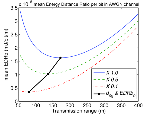
(a) AWGN channel

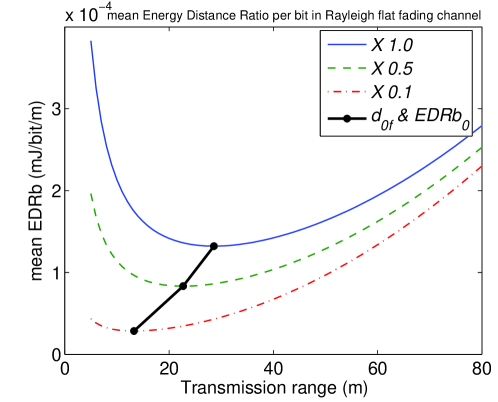
(b) Rayleigh flat fading channel

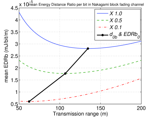
(c) Nakagami block fading channel $m=1$

Figure 6: Impact of the circuit power on the one-hop transmission energy performance given by $\overline{EDRb}$ as a function of $d$.

Fig. 6 shows the effect of circuity power on $\overline{EDRb}$ and $d_{0}$, where the whole circuity powers $P_{txElec}$, $P_{rxElec}$, $\alpha_{amp}$ and $P_{start}$ decrease by the coefficients $0.5$ and $0.1$. Since the reduction of circuity powers results in the decrease of $P_{0}$ which leads to shorten $d_{0}$. When the circuity powers are set to $0$, the shortest hop distance has the high energy efficiency [15]. Meanwhile, the energy efficiency is improved with the reduction of circuity power. Hence, the effect of circuity energy consumption should be considered in the design of WSNs.

Impact of the modulation

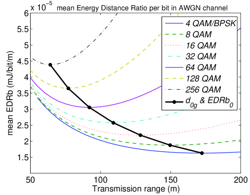
(a) AWGN channel

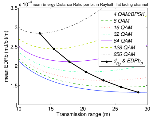
(b) Rayleigh flat fading channel

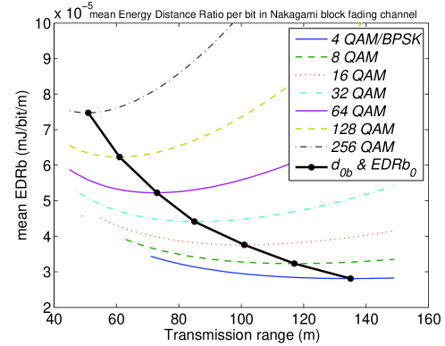
(c) Nakagami block fading channel $m=1$

Figure 7: Impact of the modulation on the one-hop transmission energy performance given by $\overline{EDRb}$ as a function of $d$.

The effect of modulation on the optimal $\overline{EDRb}$ for three kinds of channel is shown in Fig. 7. It should be noted that the optimal $\overline{EDRb}$ monotonously decreases while the optimal transmission range monotonously increases with the decrease of the order of the modulation for the three different channel types. 4QAM or BPSK are the most energy efficient among the MQAM modulations which can be explained by BER. BER increases with the order of the modulation for an identical SNR, which leads to a reduced optimal transmission range. Due to the reduction of the transmission range and duration, $E_{c}$ has a bigger proportion in the total energy consumption, which results in the increase of $\overline{EDRb}$.

Impact of the packet size

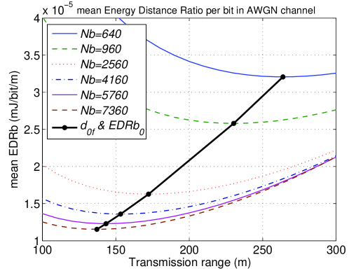
(a) AWGN channel

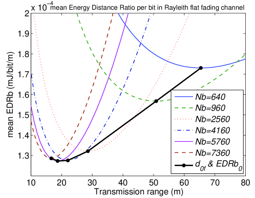
(b) Rayleigh flat fading channel

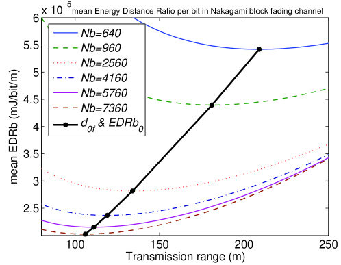
(c) Nakagami block fading channel $m=1$

Figure 8: Impact of the packet size $N_{b}$ on the one-hop transmission energy performance given by $\overline{EDRb}$ as a function of $d$.

Fig. 8 shows how the optimal $\overline{EDRb}$ varies with $N_{b}$ and the corresponding optimal transmission range for the three kinds of channel. In AWGN channel and Nakagami block fading channel, the optimal $\overline{EDRb}$ and the optimal transmission range decrease with the increase of $N_{b}$. In contrast, for Rayleigh flat fading channel, there is an optimal $N_{b}$ that originates from the trade-off between the variable transmission energy ($K_{1}\cdot P_{t}$) and $E_{c}$. The proportion of $K_{1}\cdot P_{t}$ rises in the total energy consumption with the increase of $N_{b}$, which trades off $E_{c}$. The increase of $N_{b}$ results in the decrease of the link probability, which leads to the decrease of the optimal transmission range. It can be deduced from Fig. 8 that larger packets need less energy but more hops and higher delays.

Impact of the rate

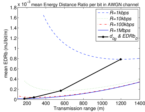
(a) AWGN channel

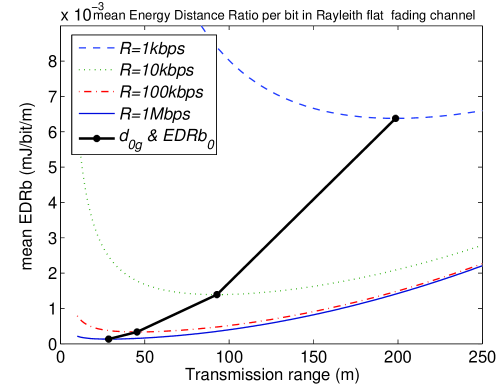
(b) Rayleigh flat fading channel

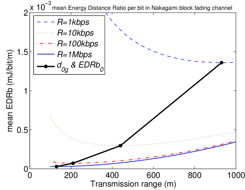
(c) Nakagami block fading channel $m=1$

Figure 9: Impact of the rate $R$ on the one-hop transmission energy performance given by $\overline{EDRb}$ as a function of $d$.

In Fig. 9, the increase of transmission rate leads to the decrease of the link probability according to Eq. (9) which brings forth the reduction of the optimal transmission range. Meanwhile, the reduction of the total energy consumption results in the decrease of the optimal $\overline{EDRb}$.

4 Multi-hop Transmission: Energy Efficiency and Delay

In this section, a multi-hop transmission along a homogeneous linear network is considered. Nodes are aligned because a transmission using properly aligned relays is more energy efficient than a transmission where the same relays do not belong to the straight line defined by the source and the destination. In this section, we first prove that the transmission along equidistant hops is the best way for saving energy in a homogeneous linear network. Next, the optimal number of hops over a homogeneous linear network is derived for a given transmission distance according to the optimal one-hop transmission distance. Finally, a lower bound on the energy efficiency and its delay is obtained for the considered multi-hop transmission.

4.1 Minimum mean total energy consumption

Theorem 1

In a homogeneous linear network, a source node $x$ sends a packet of $N_{b}$ bits to a destination node $x^{\prime}$ using $n$ hops. The distance between $x$ and $x^{\prime}$ is $d$. The length of each hop is $d_{1}$, $d_{2}$, …, $d_{n}$ respectively and the average EDRb is denoted $\overline{EDRb}(d)$. The minimum mean total energy consumption $\overline{Etot}_{min}$ is obtained for if and only if $d_{1}=d_{2}=\ldots=d_{n}$:

$$\overline{Etot}_{min}=N_{b}\cdot\overline{EDRb}(d/n)\cdot d.$$ (36)

• The mean energy consumption for each hop of index $m$ is set to $\overline{E}_{m}=N_{b}\cdot\overline{EDRb}(d_{m})\cdot d_{m},\ m=1,2,\ldots,n$. Since each hop is independent from the other hops, the mean total energy consumption is

  $$\overline{Etot}=\overline{E}_{1}+\overline{E}_{2}+\ldots+\overline{E}_{n}.$$

  Hence, the problem of finding the minimum mean total energy consumption can be rewritten as:

  minimize $$\overline{Etot}$$

  subject to $$d_{1}+d_{2}+\ldots+d_{n}=d.$$

  Set

  $$F=\overline{E}_{1}+\overline{E}_{2}+\ldots+\overline{E}_{n}+\lambda(d_{1}+d_{2}+\ldots+d_{n}-d),$$

  where $\lambda\neq 0$ is the Lagrange multiplier. According to the method of the Lagrange multipliers, we obtain

  $$\left\{\begin{split}&\frac{\partial{\overline{E_{1}}}}{\partial{d_{1}}}+\lambda=0\\ &\frac{\partial{\overline{E_{2}}}}{\partial{d_{2}}}+\lambda=0\\ &\ldots\\ &\frac{\partial{\overline{E_{n}}}}{\partial{d_{n}}}+\lambda=0\\ &d_{1}+d_{2}+\ldots+d_{n}=d\end{split}\right.$$ (37)

  Eq. (37) shows that the minimum value of $F$ is obtained in the case $\frac{\partial{\overline{E_{1}}}}{\partial{d_{1}}}=\frac{\partial{\overline{E_{2}}}}{\partial{d_{2}}}=\ldots=\frac{\partial{\overline{E_{n}}}}{\partial{d_{n}}}=-\lambda$. Moreover, in a homogeneous linear network, the properties of each node are identical. Therefore,

  $$\frac{\partial{\overline{E_{m}}}}{\partial{d_{m}}}=\frac{\partial{\overline{E}}}{\partial{d}}\bigg{|}_{d=d_{m}}$$

  where $m=1,2,\ldots,n$. Because $\frac{\partial{\overline{E}}}{\partial{d}}$ is a monotonic increasing function of $d$ when the path-loss exponent follows $\alpha\geq 2$, the unique solution of Eq. (37) is $d_{1}=d_{2}=\ldots=d_{n}=\frac{d}{n}$. Finally, we obtain:

  $$\overline{Etot}_{min}=N_{b}\cdot\overline{EDRb}(d/n)\cdot d.$$

4.2 Optimal number of hops

Based on Theorem 1 and the analysis in Section 3, the optimal hop number can be calculated from the transmission distance $d$ and the optimal one-hop transmission distance $d_{0}$. When $d/d_{0}$ is an integer, $[d/d_{0}]$ is the optimal hop number $N_{hop0}$ as each hop has the minimum $\overline{EDRb}$ according to Theorem 1. When $d/d_{0}$ is not an integer, setting $\lfloor d/d_{0}\rfloor=n$, the optimal hop number is $N_{hop0}=n\ or\ n+1$, which can be decided by:

$$Min\left\{\overline{EDRb}(d/n),\overline{EDRb}(d/(n+1))\right\}$$ (38)

where $\lfloor x\rfloor$ provides the largest integer value smaller or equal to $x$. The transmission range of each hop is now $d/N_{hop0}$.

4.3 Lower bound on $\overline{EDRb}$ and its delay

Substituting the formula $P_{0}$ and $d_{0}$ in three kinks of channel into (12) yields:

$$\overline{EDRb}=\frac{E_{c}+K_{1}P_{0}}{d_{0}p_{l}(P_{0},d_{0})}$$ (39)

Equation (39) provides the exact lower bound of $\overline{EDRb}$ on the basis of Theorem 1 and the analyzes of section 3 for a multi-hop transmission using $n$ hops. Its corresponding end-to-end delay is computed as:

$$\overline{D}_{opt}=N_{hop0}\cdot\overline{D}_{ch}$$ (40)

where $\overline{D}_{ch}$ is the one-hop transmission delays and $ch$ respectively stands for Eq. (22) with respect to AWGN channel, Eq. (28) for Rayleigh flat fading channel and Eq. (35) for Nakagami block fading channel.

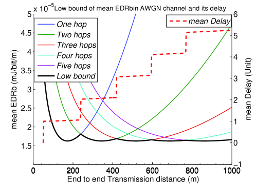
(a) AWGN channel

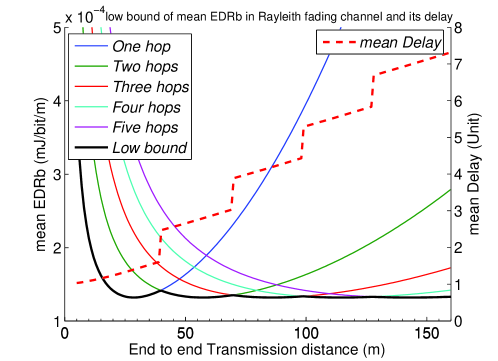
(b) Rayleigh flat fading channel

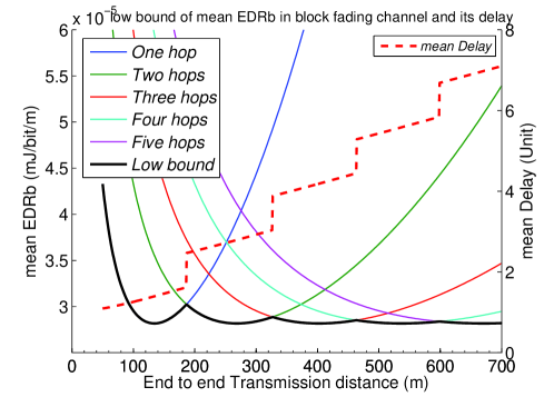
(c) Nakagami block fading channel

Figure 10: Theoretical lower bound on $\overline{EDRb}$ and the corresponding mean delay for a homogeneous linear network

Fig. 10 represents the theoretical lower bound on $\overline{EDRb}$ and its corresponding mean delay over AWGN, Rayleigh flat fading and Nakagami block fading channel. The corresponding mean delay is obtained by Eq. (40). It can be noticed that the minimum value of $\overline{EDRb}$ can be reached by following for each hop the optimum one-hop distance. It is shown in section 6 that this lower bound is also valid for 2-dimensional Poisson distributed networks using simulations.

5 Energy-Delay Trade-off

A trade-off between energy and delay exists. For instance when considering long range transmissions, a direct single-hop transmission needs a lot of energy but yields a shorter delay while a multi-hop transmission uses less energy but suffers from an extended delay as shown in Fig. 10. This section concentrates on the analyses of the energy-delay trade-off for both the one-hop and the multi-hop transmissions.

5.1 Energy-delay trade-off for one-hop transmissions

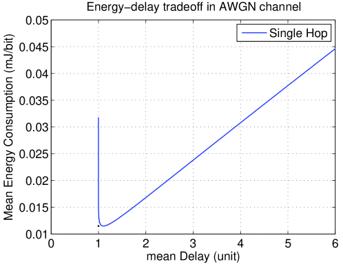
(a) AWGN channel $P_{0g}=535.87mW$

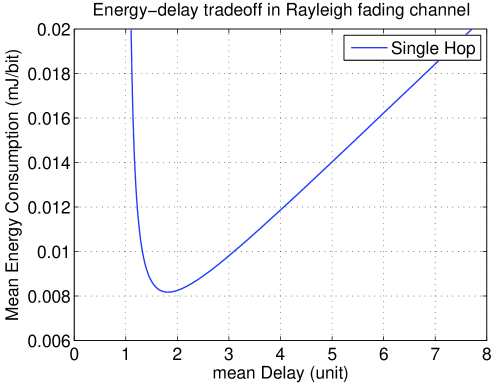
(b) Rayleigh flat fading channel $P_{0f}=734.12mW$

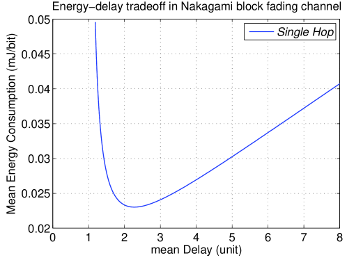
(c) Nakagami block fading channel $P_{0b}=535.87mW$

Figure 11: Energy delay trade-off for the one-hop transmission

Fig. 11 shows the energy-delay trade-off of one-hop transmission at a given distance $d=380m$ in AWGN and Nakagami block fading channel and $d=50m$ in Rayleigh flat fading channel. These three curves are obtained by varying the transmission power under this fixed transmission range. The mean delay is computed respectively using Eq. (22), (28) and (35) and the mean energy consumption is calculated by Eq. (12) over each kind of channel. The lowest points on the three curves represent the minimum energy consumptions possible for each type of channel. They correspond respectively to the energy-optimum power values $P_{0g}=535.87mW$, $P_{0f}=734.12mW$, $P_{0b}=535.87mW$ which are the same than the ones obtained with Eq. (23), (29) and (33) in section 3.

In Fig. 11, each curve can be analyzed according to the transmission power used to obtain the energy-delay value. On each curve, the points on the left of the minimum energy point are obtained with transmission powers higher than the energy-optimum power value $P_{0}$. The points on the right (i.e. experiencing higher delays) are obtained for transmission powers smaller than the energy-optimum power value $P_{0}$.

When $P_{t}$ is increasing and $P_{t}>P_{0}$, the energy consumption increases drastically while the mean delay decreases as the link gets more and more reliable. On the contrary, when $P_{t}$ is decreasing and $P_{t}<P_{0}$, the energy consumption is increasing with a slower pace while the mean delay increases as the link gets more and more unreliable. More and more retransmissions are here performed, using more energy and increasing the one-hop transmission delay.

5.2 Energy-delay trade-off for multi-hop transmissions

In section 4.2, the lower bound on the energy efficiency for a given transmission distance and its corresponding delay are analyzed determining the point of minimum energy and largest delay for a multi-hop transmission. However, in some applications subject to delay constraints, the energy consumption can be raised to diminish the transmission delay. Therefore, the energy-delay trade-off for multi-hop transmissions is analyzed in the following. To determine the energy-delay trade-off for multi-hop transmissions, we still consider a linear homogeneous network and show in Theorem 2 that the minimum mean delay is also obtained for equidistant hops.

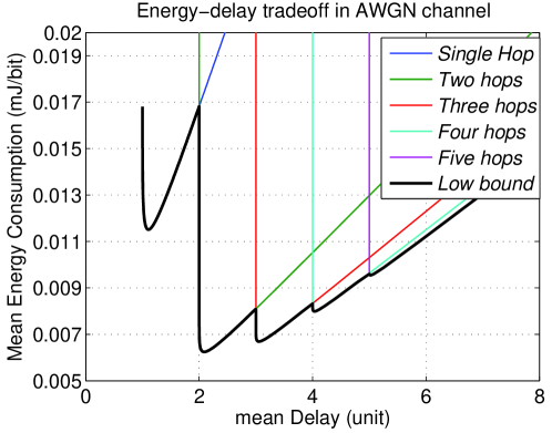
(a) AWGN channel $d=380m$

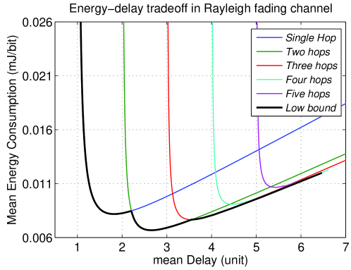
(b) Rayleigh flat fading channel $d=50m$

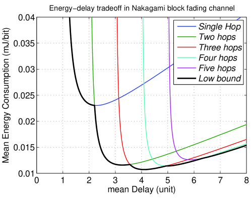
(c) Nakagami block fading channel $d=380m$

Figure 12: Energy delay trade-off for the multi-hop transmission

Theorem 2

In a homogeneous linear network, a source node $x$ sends a packet of $N_{b}$ bits to a destination node $x^{\prime}$ using $n$ hops. The distance between $x$ and $x^{\prime}$ is $d$. The length of each hop is $d_{1}$, $d_{2}$, …, $d_{n}$ respectively and the mean end to end delay is referred to as $\overline{D}(d)$. The minimum mean end to end delay $\overline{Dtot}_{min}$ is given by:

$$\overline{Dtot}_{min}=\overline{D}(d/n)\cdot n$$ (41)

if and only if $d_{1}=d_{2}=\ldots=d_{n}$.

• The mean delay of each hop is defined by $\overline{D}_{m},\ m=1,2,\ldots,n$. Since each hop is independent of the other hops, the mean end to end delay is obtained by:

  $$\overline{Dtot}=\overline{D}_{1}+\overline{D}_{2}+\ldots+\overline{D}_{n}.$$

  Hence, the problem can be rewritten as:

  minimize $$\overline{Dtot}$$

  subject to $$d_{1}+d_{2}+\ldots+d_{n}=d.$$

  We set

  $$F=\overline{D}_{1}+\overline{D}_{2}+\ldots+\overline{D}_{n}+\lambda(d_{1}+d_{2}+\ldots+d_{n}-d),$$

  where $\lambda\neq 0$ is the Lagrange multiplier. According to the method of the Lagrange multipliers, we obtain:

  $$\left\{\begin{split}&\frac{\partial{\overline{D_{1}}}}{\partial{d_{1}}}+\lambda=0\\ &\frac{\partial{\overline{D_{2}}}}{\partial{d_{2}}}+\lambda=0\\ &\ldots\\ &\frac{\partial{\overline{D_{n}}}}{\partial{d_{n}}}+\lambda=0\\ &d_{1}+d_{2}+\ldots+d_{n}=d.\end{split}\right.$$ (42)

  Eq. (42) shows that the minimum value of $F$ is obtained in the case $\frac{\partial{\overline{D_{1}}}}{\partial{d_{1}}}=\frac{\partial{\overline{D_{2}}}}{\partial{d_{2}}}=\ldots=\frac{\partial{\overline{D_{n}}}}{\partial{d_{n}}}=-\lambda$ Moreover, in a homogeneous network the properties of each node are identical. Therefore,

  $$\frac{\partial{\overline{D_{m}}}}{\partial{d_{m}}}=\frac{\partial{\overline{D}}}{\partial{d}}\bigg{|}_{d=d_{m}}$$

  where $m=1,2,\ldots,n$. Because $\frac{\partial{\overline{D}}}{\partial{d}}$ is a monotonic increasing function of $d$ when the path-loss exponent follows $\alpha\geq 2$, the unique solution of Eq. (42) is $d_{1}=d_{2}=\ldots=d_{n}=\frac{d}{n}$. Finally, we obtain:

  $$\overline{Dtot}_{min}=\overline{D}(d/n)\cdot n.$$

Based on Theorem 1 and Theorem 2, we conclude that, regarding a pair of source and destination nodes with a given number of hops, the only scenario, which minimizes both mean energy consumption and mean transmission delay, is that each hop with uniform distance along the linear path.

Fig. 12 shows the relationship between the mean energy consumption and the mean delay for a certain transmission distance in AWGN, Rayleigh and Nakagami block fading channel. The mean delay is computed with Eq. (40) and the mean energy consumption is calculated with Eq. (24), (30) and (34). According to the Theorems 1 and 2, each relay of the multi-hop transmission adopts the same transmission power according to the optimal hop distance. No maximum limit for the transmission power is considered in the computation. However, it has to be taken into account in practice.

As shown in Fig. 12, we use $d=380m$ for the AWGN and the Nakagami block fading channel and $d=50$ for the Rayleigh fading channel. Corresponding optimal number of hops is respectively $2$ hops, $2$ hops and $3$ hops respectively, which corroborates the results of Fig. 12. The bold black line gives the mean energy-delay trade-off. Knowing this particular trade-off, the routing layer can decide how many hops are needed to reach the destination under a specific transmission delay constraint.

The trade-off curve reveals the relationship between the transmission power, the transmission delay and the total energy consumption:

1. For smaller delays (fewer hops), more energy is needed due to the high transmission power needed to reach nodes located far away.

2. An increased energy consumption is not only triggered by communications with few hops but also arises for communications with several hops where the use of a reduced transmission power leads to too many retransmissions, and consequently wastes energy, too. Hence, the decrease of the transmission power does not always guaranty to a reduction of the total energy consumption.

3. For a given delay constraint, there is an optimal transmission power that minimizes the total energy consumption.

Though the lower bound on the energy-delay trade-off is derived for linear networks, it will be shown by simulations in the following section 6 that this bound is proper for 2-dimensional Poisson distributed networks.

6 Simulations in Poisson distributed networks

The purpose of this section is to determine the lower bound on the energy efficiency and on the energy-delay trade-off in a 2-dimensional Poisson distributed network using simulations. The goal is to show that the theoretical results obtained for a linear network still hold for such a more realistic scenario. We introduce this section by defining the characteristic transmission range.

6.1 Characteristic transmission range

The characteristic transmission range is defined as the range $d_{c}$ where $EDRb\_1hop(d_{c})=EDRb\_2hop(d_{c})$, i.e., the total energy consumption of a two-hop transmission is equal to that of a one-hop transmission [21] as shown in Fig. 13. In a geographical-aware network, the knowledge of $d_{c}$ at the routing layer is very useful to decide whether the optimal transmission can be done in one or two hops. Hence, when the transmission distance $d$ is greater than $d_{c}$, the use of a relay node is beneficial, on the contrary, a direct transmission is more energy efficient.

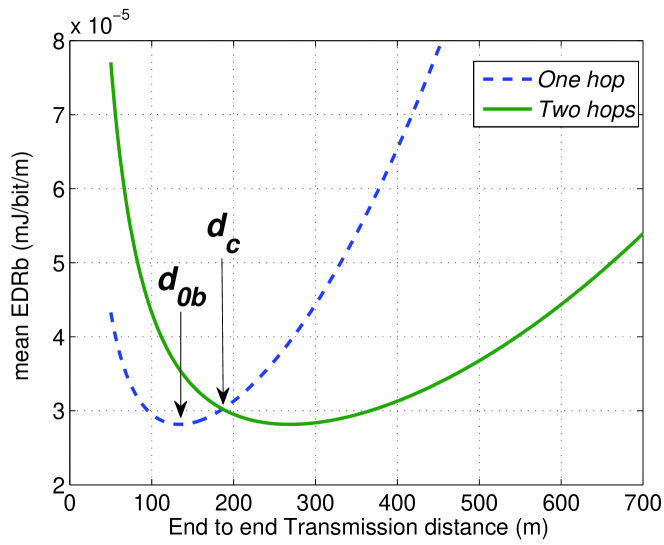
Figure 13: Characteristic Transmission Range in a Nakagami block fading channel where $d_{c}=187m$ using the related parameters listed in Table 1

6.2 Simulation setup

In the simulations, the lower bound on $\overline{EDRb}$ and on the energy-delay trade-off are evaluated in a square area $A$ of surface area $S_{A}=900\times 900m^{2}$. The nodes are uniquely deployed according to a Poisson distribution:

$$P(n\>nodes\>in\>S_{A})=\frac{(\rho\cdot S_{A})^{n}}{n!}e^{-\rho\cdot S_{A}}$$ (43)

where $\rho$ is the node density. All the other simulation parameters concerning a node are listed in Table 1. We set the node density at $\rho=0.001/m^{2}$ to ensure a full connectivity of the network [14]. The decode and forward transmission mode is adopted in the simulations.

The network model used in the simulations assumes the following statements:

• The network is geographical-aware, i.e. each node knows the position of all the nodes of the network,

• A node can adjust its transmission power according to a given transmission range, which is determined by the routing layer using Eq. (29), (23) or (33) with respect to AWGN, Rayleigh or Nakagami block fading channel respectively.

• A Time Division Multiple Access (TDMA) policy is assumed.

6.3 Simulations of the lower bound on $\overline{EDRb}$

In these simulations, a very simple routing strategy is adopted as follows:

• Step 1: The source node estimates if the distance between the source and the destination node is smaller than $d_{c}$; if YES, transmit packet directly, if NO, go to step 2.

• Step 2: Select the nodes whose distance from the source are in the range $d/N_{hop0}\pm(d_{c}-d_{0})$. If no node is chosen, expand the range step by step (size $d_{0}$) until reaching the destination node.

• Step 3: Choose the node closest to the destination node among the nodes chosen in step 2).

• Step 4: Repeat step 1) to step 3) until the destination node is reached.

In the simulations, we test all pairwise source-destination nodes. The packet size is of $2560$ bits. Then, for each pair of nodes, we calculate the end to end energy consumption and its Euclidean distance. The simulation is implemented for $1500$ times, $600$ times and $100$ times respectively corresponding to the node density $0.0001node/m^{2}$, $0.0002node/m^{2}$ and $0.001node/m^{2}$.

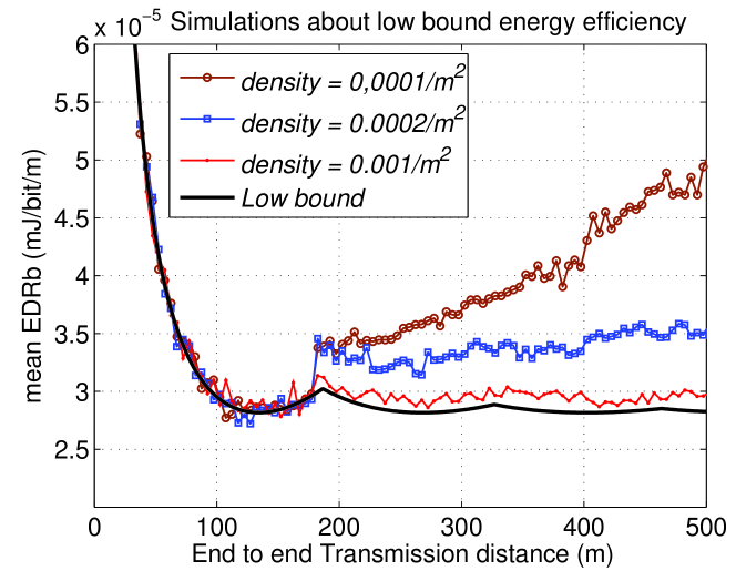
Figure 14: Simulation results for the energy efficiency $\overline{EDRb}$ in Nakagami block fading channel, m =1.

Fig. 14 shows the simulation results for the energy efficiency $\overline{EDRb}$ considering different node densities, a Nakagami block fading channel and a BPSK modulation. We have $d_{0}b=134.16m$ and $d_{c}=187m$ in this case. These results show that:

1. The theoretical lower bound on $\overline{EDRb}$ is adequate to a 2-D Poisson network although its derivation is based on a linear network.

   When the node density is of $0.001/m^{2}$, the theoretical lower bound and the one obtained by simulations coincide. For this density, a full connectivity of the network exists. Hence, we can conclude that our theoretical lower bound for the average energy efficiency is suitable for Poisson networks. When the node density is reduced, theoretical and simulation based curves for the mean $\overline{EDRb}$ diverge when the end to end transmission distance $d$ increases. In that case, the source node can not find a relay node in the optimal transmission range and has to search for a further relay node which increases the energy consumption.

2. Unreliable links play an important role for energy savings.

   In the simulations, the transmission power is adapted according to the transmission distance on the basis of the analysis of Section 3. Hence, unreliable links also contribute to attain the lower bound on $\overline{EDRb}$ (as presented in Fig. 2 and 3, the optimal link probability is about $0.72$).

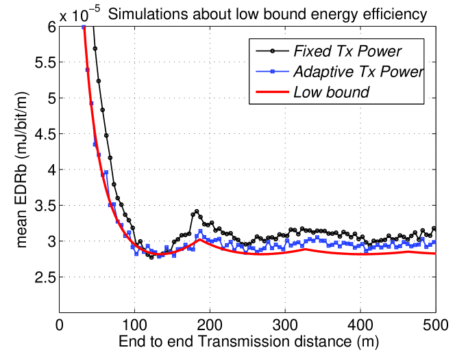
Figure 15: Simulation results for $\overline{EDRb}$ in Nakagami block fading channel using fixed transmission. Here, the node density is $0.001/m^{2}$, m=1.

Adaptive transmission power is not available in many cheap sensor nodes. Therefore, we consider a fixed transmission power for each node in the simulation which is set to the energy-optimal transmission power of Eq. (16). Simulation results for a fully connected network are shown in Fig. 15. Compared to the adaptive transmission power mode, nodes with fixed transmission power show a slightly higher $\overline{EDRb}$, i.e., lower energy efficiency. Nevertheless, the advantage in terms of simplicity due to the use of fixed transmission powers makes it worthwhile the little increase in energy consumption.

6.4 Simulations of the energy-delay trade-off

The simulations regarding the energy-delay trade-off are also implemented for a Nakagami block fading channel and for a fixed end-to-end transmission distance of $380m$. Regarding each pairs of nodes, the source nodes try to use $1$ to $5$ hops in turn.

The following relay selection strategy is adopted knowing the number of hops:

• Step 1: Calculate the hop range according to the hop number, i.e., $380m/hop\ number$.

• Step 2: Select the set of relay nodes that belong to the 1-hop transmission range (1-hop length). If the set of relay nodes is empty, extend the range by 1-hop length until reaching the destination node.

• Step 3: Choose the node closest to the destination node among the nodes chosen in step 2).

• Step 4: Repeat Step 2) and Step 3) until the destination node is reached, then, return selected relay node.

The source node and the selected relay node(s) will transmit the packet with the same transmission power and the value of transmission power starts form $1dBm$ and increases by $1dBm$ until $40dBm$. Each simulation is repeated 50 times. Then, we compute the delay and the energy consumption for each routing. Finally we obtain the mean delay and mean energy consumption for the same hop number. In this way, we obtain the low bound of energy-delay trade-off for three different node densities.

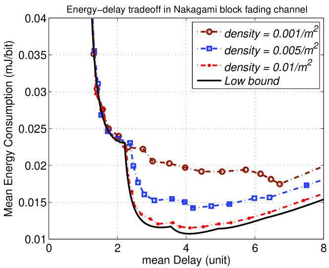
Figure 16: Simulation results for the energy-delay trade-off in Nakagami block fading channel, m =1.

In Fig. 16, simulation results are given for different node densities. For a node density of $0.01/m^{2}$, the lower bound on the energy delay trade-off is reached since there are enough nodes to find a suitable relay given the delay constraint. This result indicates that the theoretical lower bound on the energy-delay trade-off is valid for a Poisson network though its derivation is based on a linear network. For smaller node densities, the energy delay trade-off obtained by simulations diverges from the lower bound since non energy-optimal relays have to be used which increases the energy consumption and the transmission delay.

7 Conclusions

This paper, using realistic unreliable link model, explores the low bound of energy-delay trade-off in AWGN channel, Rayleigh flat fading channel and Nakagami block fading channel. Firstly, we propose a metric for energy efficiency, $\overline{EDRb}$, which is combined with the unreliable link model. It reveals the relation between the energy consumption of a node and the transmission distance which may contribute to determine optimal route at the routing layer. By optimizing $\overline{EDRb}$, a closed form expression of the energy-optimal transmission range is obtained for AWGN, Rayleigh flat fading and Nakagami block fading channel. Based on this optimal transmission range, the lower bound on $\overline{EDRb}$ for a multi-hop transmission using a linear network is derived for the three different kinds of channel. In addition, the lower bound on the energy-delay trade-off is studied for the same multi-hop transmission over a linear network. Results are then validated using simulations of a 2-D Poisson distributed network. Theoretical analyses and simulations show that accounting for unreliable links in the transmission contributes to improve the energy efficiency of the system under delay constraints, especially for Rayleigh flat fading and Nakagami block fading channel.

Appendix A Derivation of $P_{0}$ and $d_{0}$

Substituting (8) and (9) into (14) and (15), we obtain:

$$\left\{\begin{split}&\frac{d^{\alpha}K_{1}p_{l}(\gamma)-K_{2}(E_{c}+K_{1}P_{t})p_{l}^{\prime}(\gamma)}{d^{(\alpha+1)}p_{l}^{2}(\gamma)}&=0\\ &\frac{(E_{c}+K_{1}P_{t})\cdot(-d^{\alpha}p_{l}(\gamma)+K_{2}P_{t}\alpha p_{l}^{\prime}(\gamma))}{d^{(\alpha+2)}p_{l}^{2}(\gamma)}&=0\end{split}\right.$$ (44)

where $p_{l}^{\prime}(\gamma)$ is the derivative of the function $p_{l}(\gamma)$. Because $E_{c}+K_{1}P_{t}$ is greater than $0$, simplifying the equation set (44) yields:

$$\left\{\begin{split}&d^{\alpha}K_{1}p_{l}(\gamma)-K_{2}(E_{c}+K_{1}P_{t})p_{l}^{\prime}(\gamma)&=0\\ &-d^{\alpha}p_{l}(\gamma)+K_{2}P_{t}\alpha p_{l}^{\prime}(\gamma)&=0\end{split}\right.$$ (45)

Solving the equation set (45) and substituting $\gamma$ with (9), we have:

$$P_{0}=\frac{E_{c}}{K_{1}(\alpha-1)}$$

and

$$d_{0}^{\alpha}=\frac{p_{l}^{\prime}(K_{2}P_{0}d_{0}^{-\alpha})K_{2}P_{0}}{p_{l}(K_{2}P_{0}d_{0}^{-\alpha})}.$$

Appendix B Derivation of the optimal transmission range in AWGN channel

According to (8), the link model in AWGN channel is given by:

$$p_{l}=(1-BER(\gamma))^{N_{b}},$$ (46)

where $BER(\gamma)$ is the Bit Error Rate (BER). A closed form of BER is described in [22] for coherent detection in AWGN channel:

$$BER(\gamma_{b})=\alpha_{m}{\textrm{Q}}(\sqrt{\beta_{m}\gamma_{b}}),$$ (47)

with the Q function, $\textrm{Q}(x)=\int_{x}^{\infty}\frac{1}{\sqrt{\pi}}e^{-u^{2}/2}du$, where $\alpha_{m}$ and $\beta_{m}$ rely on the modulation type and order, e.g., for Multiple Quadrature Amplitude Modulation (MQAM) $\alpha_{m}=4(1-1/\sqrt{M})/\log_{2}(M)$ and $\beta_{m}=3\log_{2}(M)/(M-1)$ . For Binary Phase Shift Keying (BPSK), $\alpha_{m}=1$ and $\beta_{m}=2$.

The closed form expression of $d_{0}$ can not be obtained using the exact $BER(\gamma)$. A simplified tight approximation of $BER(\gamma)$ is obtained when $\beta_{m}\cdot\gamma_{b}\geq 2$ by using the method proposed in [23]:

$$BER_{g}(\gamma_{b})\approx 0.1826\alpha_{m}\cdot\exp(-0.5415\beta_{m}\gamma_{b})\ \ \ \text{i}f\ \beta_{m}\cdot\gamma_{b}\geq 2,$$ (48)

where $\exp(\cdot)$ represents the exponential function. Fig. 17 shows the relation between the approximation and the exact values of the BER.

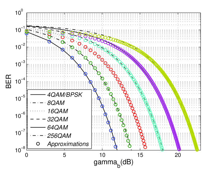
Figure 17: BER approximations for MQAM

Therefore, the optimal transmission range $d_{0g}$ is obtained by substituting (48) and (16) into (15):

$$d_{0g}=\left(\frac{-0.5415\beta_{m}K_{2}N_{b}E_{c}\alpha}{K_{1}(\alpha-1)(1+\alpha N_{b}\text{W}_{-1}\left[\frac{-e^{-\frac{1}{N_{b}\cdot\alpha}}}{0.1826\alpha_{m}N_{b}\alpha}\right])}\right)^{\frac{1}{\alpha}},$$ (49)

where $\text{W}_{-1}[\cdot]$ is the branch satisfying $\text{W}(x)<-1$ of the Lambert W function [18].

Appendix C Derivation of the optimal transmission range in Rayleigh flat fading channel

There is a general expression for the BER in Rayleigh flat fading channel in case of $\bar{\gamma}\geq 5$ in [22]:

$$BER_{f}(\bar{\gamma})\approx\frac{\alpha_{m}}{2\beta_{m}\bar{\gamma}}$$ (50)

where $\alpha_{m}$ and $\beta_{m}$ are the same as those in (48).

Substituting (50) and (9) into (12), we have:

$$\overline{EDRb_{f}}(d,P_{t})=\frac{E_{c}+K_{1}\cdot P_{t}}{d\left(1-\frac{\alpha_{m}}{2\beta_{m}K_{2}\cdot P_{t}\cdot d^{-\alpha}}\right)^{N_{b}}}$$ (51)

Substituting (51) and (16) into (14), the optimal transmission range $d_{0f}$ in Rayleigh flat fading channel is obtained:

$$d_{0f}=\left(\frac{2\beta_{m}E_{c}\cdot{K_{2}}}{(\alpha-1)\cdot{K_{1}}\alpha_{m}(\alpha N_{b}+1)}\right)^{\frac{1}{\alpha}}$$ (52)

Appendix D Derivation of the optimal transmission range in Nakagami block fading channel

The exact link model in Nakagami block fading channel is [14]:

$$p_{l}(\bar{\gamma})=\int_{\gamma=0}^{\infty}(1-BER(\gamma))^{N_{b}}p(\gamma|\bar{\gamma})d\gamma,$$ (53)

where

$$p(\gamma|\bar{\gamma})=\frac{m^{m}\gamma^{m-1}}{\bar{\gamma}\Gamma(m)}\exp\left(-\frac{m\gamma}{\bar{\gamma}}\right),$$ (54)

$BER(\gamma)$ refers to (48).

When $m=1$ (Rayleigh block fading) and $\alpha_{m}=1$, the approximation of (53) is found:

$$pl(\overline{\gamma})=\exp\left(\frac{-4.25\log_{10}(Nb)+2.2}{\beta_{m}\overline{\gamma}}\right).$$ (55)

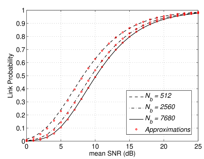
Figure 18: Approximations of link probability for Rayleigh block fading

Fig. 18 shows the approximations for different values of $N_{b}$.

Substituting (55) and (16) into (14) yields the optimal transmission range $d_{0b}$:

$$d_{0b}=\left(\frac{\beta_{m}K_{2}E_{c}}{K_{1}(\alpha^{2}-\alpha)(4.25\log_{10}(N_{b})-2.2)}\right)^{1/\alpha}.$$ (56)

Contents

1. 1 Introduction
2. 2 Models and Metric
   1. 2.1 Energy consumption model
   2. 2.2 Realistic unreliable link model
   3. 2.3 Mean energy distance ratio per bit ($\overline{EDRb}$)
   4. 2.4 Delay model
3. 3 One-hop Transmission: Energy Efficiency and Delay
   1. 3.1 Energy-optimal transmission power $P_{0}$
   2. 3.2 Energy-optimal transmission range $d_{0}$ and its delay
      1. 3.2.1 AWGN channel
      2. 3.2.2 Rayleigh flat fading channel [19]
      3. 3.2.3 Nakagami block fading channel
   3. 3.3 Impact of some physical parameters
4. 4 Multi-hop Transmission: Energy Efficiency and Delay
   1. 4.1 Minimum mean total energy consumption
   2. 4.2 Optimal number of hops
   3. 4.3 Lower bound on $\overline{EDRb}$ and its delay
5. 5 Energy-Delay Trade-off
   1. 5.1 Energy-delay trade-off for one-hop transmissions
   2. 5.2 Energy-delay trade-off for multi-hop transmissions
6. 6 Simulations in Poisson distributed networks
   1. 6.1 Characteristic transmission range
   2. 6.2 Simulation setup
   3. 6.3 Simulations of the lower bound on $\overline{EDRb}$
   4. 6.4 Simulations of the energy-delay trade-off
7. 7 Conclusions
8. A Derivation of $P_{0}$ and $d_{0}$
9. B Derivation of the optimal transmission range in AWGN channel
10. C Derivation of the optimal transmission range in Rayleigh flat fading channel
11. D Derivation of the optimal transmission range in Nakagami block fading channel

References

- [1] A. J. Goldsmith and S. B. Wicker, “Design challenges for energy-constrained ad hoc wireless networks,” Wireless Communications, IEEE [see also IEEE Personal Communications], vol. 9, no. 4, pp. 8–27, 2002.
- [2] M. Haenggi and D. Puccinelli, “Routing in ad hoc networks: a case for long hops,” Communications Magazine, IEEE, vol. 43, no. 10, pp. 93–101, 2005.
- [3] P. Chen, B. O’Dea, and E. Callaway, “Energy efficient system design with optimum transmission range for wireless ad hoc networks,” in Communications, 2002. ICC 2002. IEEE International Conference on, vol. 2, pp. 945–952, 2002.
- [4] J. L. Gao, “Analysis of energy consumption for ad hoc wireless sensor networks using a bit-meter-per-joule metric,” tech. rep., 2002.
- [5] J. Deng, Y. S. Han, P. N. Chen, and P. K. Varshney, “Optimal transmission range for wireless ad hoc networks based on energy efficiency,” Communications, IEEE Transactions on, vol. 55, no. 7, pp. 1439–1439, 2007.
- [6] S. Cui, R. Madan, A. J. Goldsmith, and S. Lall, “Cross-layer energy and delay optimization in small-scale sensor networks,” Wireless Communications, IEEE Transactions on, vol. 6, no. 10, pp. 3688–3699, 2007.
- [7] M. Haenggi, “On routing in random rayleigh fading networks,” Wireless Communications, IEEE Transactions on, vol. 4, no. 4, pp. 1553–1562, 2005.
- [8] S. Cui, R. Madan, A. Goldsmith, and S. Lall, “Energy-delay tradeoffs for data collection in tdma-based sensor networks,” in Communications, 2005. ICC 2005. 2005 IEEE International Conference on, vol. 5, pp. 3278–3284, 2005.
- [9] S. Y. Chang, “Energy-delay analysis of wireless networks over rayleigh fading channel,” in Wireless Telecommunications Symposium, 2005, pp. 197–201, 2005.
- [10] D. Ganesan, B. Krishnamachari, A. Woo, D. Culler, D. Estrin, and S. Wicker, “Complex behavior at scale: An experimental study of low-power wireless sensor networks,” tech. rep., 2003.
- [11] A. Woo and D. E. Culler, “Evaluation of efficient link reliability estimators for low-power wireless networks,” tech. rep., Computer Science Division, University of California, 2003.
- [12] J. Zhao and R. Govindan, “Understanding packet delivery performance in dense wireless networks,” in Proceedings of the 1st international conference on Embedded networked sensor systems, (Los Angeles, California, USA), pp. 1–13, ACM Press, 2003.
- [13] M. Z. Zamalloa and K. Bhaskar, “An analysis of unreliability and asymmetry in low-power wireless links,” ACM Transactions on Sensor Networks, vol. 3, no. 2, p. 7, 2007.
- [14] J.-M. Gorce, R. Zhang, and H. Parvery, “Impact of radio link unreliability on the connectivity of wireless sensor networks,” EURASIP Journal on Wireless Communications and Networking, vol. 2007, 2007.
- [15] S. Banerjee and A. Misra, “Energy efficient reliable communication for multi-hop wireless networks,” Journal of Wireless Networks (WINET), 2004.
- [16] H. Karl and A. Willig, Protocols and Architectures for Wireless Sensor Networks. John Wiley and Sons, 2005.
- [17] M. Haenggi, “The impact of power amplifier characteristics on routing in random wireless networks,” in Global Telecommunications Conference, 2003. GLOBECOM ’03. IEEE, vol. 1, pp. 513–517, 2003.
- [18] R. Corless, G. Gonnet, D. Hare, D. Jeffrey, and D. Knuth, “On the lambertw function,” Advances in Computational Mathematics, vol. 5, no. 1, pp. 329–359, 1996.
- [19] R. Zhang and J.-M. Gorce, “Optimal transmission range for minimum energy consumption in wireless sensor networks,” in IEEE WCNC, (Las Vegas, USA), 2008.
- [20] A. Ravindran, K. M. Ragsdell, and G. V. Reklaitis, Engineering Optimization. Wiley, second ed., 2006.
- [21] R. Min, M. Bhardwaj, N. Ickes, A. Wang, and A. Chandrakasan, “The hardware and the network: Total-system strategies for power aware wireless microsensors,” in Proc. IEEE CAS Workshop on Wireless Communications and Networking, 2002.
- [22] A. Goldsmith, Wireless Communications. cambridge university press, 2005.
- [23] N. Ermolova and S. G. Haggman, “Simplified bounds for the complementary error function; application to the performance evaluation of signal-processing systems,” in EUSIPCO 2004 : (XII. European Signal Processing Conference), (Vienna, Austria), 2004.