Abstract

Within the Hamiltonian approach in Coulomb gauge the ghost and gluon propagators are determined from a variational solution of the Yang–Mills Schrödinger equation showing both gluon and heavy quark confinement. The continuum results are in good agreement with lattice data. The ghost form factor is identified as the dielectric function of the Yang–Mills vacuum and a connection between the Gribov–Zwanziger scenario and the dual Meissner effect is established. The topological susceptibility is calculated.

1 Introduction

The aim of the talk is the microscopic description of infrared properties of QCD like confinement. We would like to see, for example, the emergence of the colour flux string between static colour charges. For this purpose, I will use the Hamiltonian approach to Yang-Mills theory in Coulomb gauge. The organisation of my talk is as follows: In section 2, I will briefly summarise the essential ingredients of the Hamiltonian approach to Yang-Mills theory in Coulomb gauge. Then I will present a variational solution of the Yang-Mills Schrödinger equation in section 3, which will result in a set of coupled Dyson-Schwinger equations. I will present the analytic solutions to these equations in the infrared and ultraviolet and the numerical solution for the full momentum range. The resulting propagators will then be compared to the available lattice data. Then I will focus on two non-perturbative properties of the Yang-Mills vacuum: the dielectric constant in section 4 and the topological susceptibility in section 5. Finally, a summary is provided.

2 Canonical quantisation of Yang-Mills theory

In the canonical quantisation approach the gauge fields $A^{a}_{\mu}(x)$ are considered as the (cartesian) coordinates and the corresponding conjugate momenta are defined by

$$\Pi^{a}_{\mu}(x)=\frac{\delta S}{\delta\partial_{0}A^{a}_{\mu}(x)}\hskip 2.84544pt,$$ (1)

where $S$ is the action of the Yang-Mills field. The explicit calculation yields

$$\Pi^{a}_{i}(x)=E^{a}_{i}(x)\hskip 2.84544pt,\hskip 2.84544pt\Pi^{a}_{0}(x)=0\hskip 2.84544pt,$$ (2)

where $E^{a}_{i}(x)$ is the colour electric field. To avoid the problems arising from the vanishing temporal component of the canonical momentum, one imposes Weyl gauge $A^{a}_{0}(x)=0$. The Yang-Mills Hamiltonian is then given by

$$H=\frac{1}{2}\int d^{3}x\left(\mbox{\boldmath$\Pi$\unboldmath}^{2}(x)+{\mbox{\boldmath$B$\unboldmath}}^{2}(x)\right)\hskip 2.84544pt.$$ (3)

The canonical quantisation is carried out in the standard fashion by imposing the canonical commutation relation $[A^{a}_{i}(x),\Pi^{b}_{j}(y)]=\delta_{ij}\delta^{ab}\delta^{3}(x-y)$, which promotes the canonical momentum to the operator $\Pi^{a}_{i}(x)=\delta/i\delta A^{a}_{i}(x)$. By imposing Weyl gauge one loses Gauss’ law from the Heisenberg equation of motion and Gauss’ law has to be imposed as a constraint on the wave functional

$${\bf\hat{D}\cdot\Pi}(x)\psi(x)=-g\rho_{m}(x)\psi(x)\hskip 2.84544pt,$$ (4)

where $\rho_{m}(x)$ is the colour charge density of the matter fields and $\hat{D}^{ab}_{i}=\delta^{ab}\partial_{i}+g\hat{A}^{ab}_{i}\hskip 2.84544pt\;$ $(\hat{A}^{ab}=f^{acb}A^{c}$) is the covariant derivative in the adjoint representation of the gauge field with $f^{abc}$ being the structure constant of the gauge group. The operator on the left hand side of Gauss’ law is nothing but the generator of time-independent gauge transformations and in the absence of external colour charges, $\rho_{m}(x)=0$, Gauss’ law expresses the invariance of the wave functional under space-dependent but time-independent gauge transformations.

Instead of working with explicit gauge invariant wave functionals it is more convenient to explicitly resolve Gauss’ law by fixing the gauge. Coulomb gauge is a particular convenient choice for this purpose. We implement the Coulomb gauge, $\mbox{\boldmath$\partial$\unboldmath}\cdot{\mbox{\boldmath$A$\unboldmath}}=0$, in the standard fashion into the scalar product of the wave functionals by means of the Faddeev-Popov method

$$\langle\psi|{\cal{O}}|\phi\rangle=\int DA^{\perp}J(A^{\perp})\psi^{*}(A^{\perp}){\cal{O}}[A^{\perp}]\phi(A^{\perp})\hskip 2.84544pt,$$ (5)

where

$$J=\mathrm{Det}(-\mbox{\boldmath$\hat{D}$\unboldmath}\cdot\mbox{\boldmath$\partial$\unboldmath})$$ (6)

is the Faddeev-Popov determinant. While in Coulomb gauge the gauge field is transversal the momentum operator $\mbox{\boldmath$\Pi$\unboldmath}=\mbox{\boldmath$\Pi$\unboldmath}^{||}+\mbox{\boldmath$\Pi$\unboldmath}^{\perp}$ contains both longitudinal $\mbox{\boldmath$\Pi$\unboldmath}^{||}$ and transversal $\mbox{\boldmath$\Pi$\unboldmath}^{\perp}$ parts. Resolving Gauss’ law for the longitudinal part of the momentum operator yields

$$\mbox{\boldmath$\Pi$\unboldmath}^{||}\psi=g\mbox{\boldmath$\partial$\unboldmath}(-\mbox{\boldmath$\hat{D}$\unboldmath}\cdot\mbox{\boldmath$\partial$\unboldmath})^{-1}\rho\,\psi\hskip 2.84544pt,\hskip 2.84544pt\rho=\rho_{g}+\rho_{m}\hskip 2.84544pt,$$ (7)

where

$$\rho_{g}={\bf\hat{A}^{\perp}\cdot\Pi^{\perp}}$$ (8)

is the colour charge density of the gauge field. With this result the Hamiltonian in Coulomb gauge is found to be

$$H=\frac{1}{2}\int\left(J^{-1}\mbox{\boldmath$\Pi$\unboldmath}^{\perp}J\mbox{\boldmath$\Pi$\unboldmath}^{\perp}+{\mbox{\boldmath$B$\unboldmath}}^{2}\right)+H_{C}\hskip 2.84544pt,$$ (9)

where

$$H_{C} = \frac{1}{2}\int J^{-1}\mbox{\boldmath$\Pi$\unboldmath}^{\parallel}J\mbox{\boldmath$\Pi$\unboldmath}^{\parallel}=\frac{g^{2}}{2}\int J^{-1}\rho(-\mbox{\boldmath$\hat{D}$\unboldmath}\cdot\mbox{\boldmath$\partial$\unboldmath})^{-1}(-\mbox{\boldmath$\partial$\unboldmath}^{2})(-\mbox{\boldmath$\hat{D}$\unboldmath}\cdot\mbox{\boldmath$\partial$\unboldmath})^{-1}J\rho\hskip 2.84544pt$$ (10)

is the so-called Coulomb Hamiltonian, which arises from the longitudinal part of the kinetic energy after resolving Gauss’ law. The Hamiltonian (9) was first derived in Ref. [1].

3 Variational solution

Figure 1: Ghost form factor $d(k)$ (left) and gluon energy $\omega(k)$ from the variational solutions presented in [2].

We wish to solve the Schrödinger equation

$$H\psi=E\psi$$ (11)

by the variational principle

$$\langle\psi|H|\psi\rangle\to min\hskip 2.84544pt$$ (12)

with suitable ansätze for the wave functional $\psi(A^{\perp})$. This approach has been studied resently in Refs. [3, 4]. Inspired by the wave functional of a massless particle moving in a spherically symmetric potential in an $s$-state $\psi=\phi(r)/r$, where $r={J^{1/2}(r)}$ is the Jacobian of the transformation from the cartesian to the spherical coordinates for zero angular momentum we choose the following ansatz [4]

$$\psi(A^{\perp})=\frac{1}{\sqrt{J(A^{\perp})}}\exp\left(-\frac{1}{2}\int d^{3}xd^{3}yA^{\perp a}_{i}(x)\omega(x,y)A^{\perp a}_{i}(y)\right)\hskip 2.84544pt,$$ (13)

where the kernel $\omega(x,y)$ is determined from the variational principle (12). In practice the so resulting equation for $\omega(x,y)$ is converted into a set of Dyson-Schwinger equations for the gluon propagator

$$\langle A^{\perp a}_{i}(x)A^{\perp b}_{j}(y)\rangle=\delta^{ab}t_{ij}(x)\frac{1}{2}\omega^{-1}(x,y)\;,$$ (14)

with $t_{ij}(x)=\delta_{ij}-\frac{\partial_{i}\partial_{j}}{\partial^{2}}$ being the transverse projector, and the ghost propagator

$$G(x,y)=\left\langle\left(-\mbox{\boldmath$\hat{D}$\unboldmath}\cdot\mbox{\boldmath$\partial$\unboldmath}\right)^{-1}\right\rangle=\langle x|d(-\Delta)(-\Delta)^{-1}|y\rangle\hskip 2.84544pt.$$ (15)

Here we have introduced the ghost form factor $d(-\Delta)$, which describes the deviation of the QCD ghost propagator from the QED case, where $d(-\Delta)\equiv 1$. The resulting Dyson-Schwinger equations need renormalisation, which is well under control. Fig. 1 shows the solution of the Dyson-Schwinger equation for the gluon energy $\omega(k)$ and the ghost form factor $d(k)$, as shown in Ref. [2]. An analytic infrared and ultraviolet analysis of the Dyson-Schwinger equation shows the following asymptotic behaviour [4, 5]

$$\mathrm{IR}\,(k\to 0) : \omega(k)\sim\frac{1}{k}\hskip 28.45274ptd(k)\sim\frac{1}{k}$$

$$\mathrm{UV}\,(k\to\infty) : \omega(k)\sim{k}\hskip 28.45274ptd(k)\sim k^{0}\hskip 2.84544pt.$$ (16)

At large momenta the gluon behaves like a photon, which is in agreement with asymptotic freedom, while at small momenta the gluon energy diverges, which implies the absence of gluon states in the physical spectrum. This is nothing but a manifestation of gluon confinement. The infrared divergence of the ghost form factor is a consequence of the horizon condition

$$d^{-1}(k=0)=0\hskip 2.84544pt,$$ (17)

which has been used as input in the renormalisation of the ghost Dyson-Schwinger equation. This is a necessary condition for the Gribov-Zwanziger confinement scenario. In fact, one can show there is a sum rule relating the infrared exponents of the ghost and the gluon propagator and an infrared divergent gluon energy requires also an infrared divergent ghost form factor, i.e. the horizon condition (17), see Ref. [5].

Figure 2: Left: Heavy quark potential given by eq. (18). Right: Running coupling constant.

Fig. 2 shows the non-Abelian Coulomb potential

$$V(|x-y|)=g^{2}\left\langle\langle x|(-\mbox{\boldmath$\hat{D}$\unboldmath}\cdot\mbox{\boldmath$\partial$\unboldmath})^{-1}(-\mbox{\boldmath$\partial$\unboldmath}^{2})(-\mbox{\boldmath$\hat{D}$\unboldmath}\cdot\mbox{\boldmath$\partial$\unboldmath})^{-1}|y\rangle\right\rangle\rightarrow\sigma_{C}\,|x-y|\hskip 2.84544pt,$$ (18)

which for large distance indeed increases linearly [2] as the infrared analysis reveals. The Coulomb string tension $\sigma_{C}$ sets the scale of our approach. Also shown in Fig. 2 is the running coupling constant which is infrared finite, for details see Ref. [5]. Fig. 3 shows the continuum results for the gluon energy and the ghost form factor in $D=2+1$ dimensions [6] together with the corresponding lattice results, Ref. [7]. The agreement is not perfect but, given the approximation involved, quite satisfactory.

In $D=3+1$ dimensions, previous lattice calculations performed in Coulomb gauge in Ref. [8, 9] showed an anomalous UV behaviour of the gluon propagator — $\mathrm{IR}:\omega(k)\sim k^{0}\,,\;\mathrm{UV}:\omega(k)\sim k^{3/2}$ — which is in strong conflict with the continuum result. However, one should mention that these lattice calculations assumed multiplicative renormalisability of the 4-dimensional gluon propagator, which give rise to scaling violations in the static propagator. Furthermore, these calculations did not fix the gauge completely, i.e. the residual time-dependent gauge invariance left after Coulomb gauge fixing was left unfixed. Furthermore, the Coulomb gauge fixing was done on a single time-slice, which is sufficient for the calculation of static (time-independent) propagators. However, one should keep in mind that in Coulomb gauge topologically non-trivial gauge configurations, which presumably are responsible for confinement, are discontinuous in time [10] and as a consequence on a small lattice different results are obtained from different time slices.

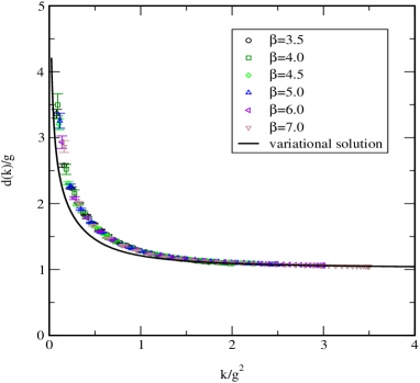
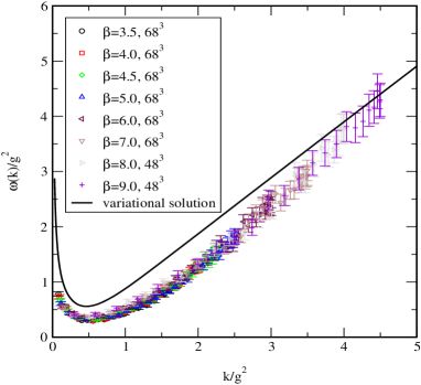
Figure 3: Results for the ghost form factor $d(k)$ (left) and the gluon energy $\omega(k)$ in $2+1$ dimensions, as shown in [6].

Recently, we have done improved lattice calculations with a complete gauge fixing [11]. In these studies, the energy dependence of the 4-dimensional gluon propagator could be explicitly extracted and it was found that the static gluon propagator is multiplicatively renormalisable and shows a perfect scaling. Fig. 4 (left panel) shows the results for the gluon propagator of these calculations together with the continuum results. It is assumed here that the Coulomb string tension $\sigma_{C}$ is identical to the string tension $\sigma$ from the Wilson loop. There is a very good agreement, in particular the ultraviolet and infrared behaviour matches perfect for lattice and continuum. What is also remarkable that the lattice result can be very well fitted by Gribov’s original formula for the gluon energy

$$\omega(k)=\sqrt{k^{2}+\frac{M^{4}}{k^{2}}}$$ (19)

with $M=0.88(1)\,\mathrm{GeV}$.

Figure 4: Left: Lattice data for $\omega(k)$, compared to the solution of the Dyson-Schwinger equations. Right: Dielectric function $\epsilon(k)$.

4 The colour dielectric constant

Consider the electric field generated by a charge density $\rho$ in electrodynamics

$${\bf E}=-\mbox{\boldmath$\partial$\unboldmath}\phi\hskip 2.84544pt,\hskip 2.84544pt\phi=(-\Delta)^{-1}\rho\hskip 2.84544pt.$$ (20)

The longitudinal electric field resulting from the resolution of Gauss’ law in the Yang-Mills case is given by a similar expression

$${\bf E} = \langle{\bf\Pi}\rangle=-\partial\phi\hskip 2.84544pt$$

$$\phi = \left\langle\left(-\mbox{\boldmath$\hat{D}$\unboldmath}\cdot\mbox{\boldmath$\partial$\unboldmath}\right)^{-1}\right\rangle\rho=d(-\Delta)(-\Delta)^{-1}\rho\hskip 2.84544pt$$ (21)

except that the Green’s function of the Laplacian is replaced by the ghost propagator (15). The last expression has the form of the scalar potential in the presence of a dia-electric medium

$$\phi=\epsilon^{-1}(-\Delta)^{-1}\rho$$ (22)

and the inverse of the ghost form factor $d(k)$ can thus be identified as the dielectric function of the Yang-Mills vacuum

$$\epsilon(k)=d^{-1}(k)\hskip 2.84544pt.$$ (23)

Fig. 4 (right panel) shows the so defined dielectric function. It satisfies $0<\epsilon(k)<1$, which is a manifestation of anti-screening while in QED we have $\epsilon(k)>1$, which corresponds to ordinary Debye screening. Furthermore, at zero momentum the dielectric function vanishes, showing that in the infrared the Yang-Mills vacuum behaves like a perfect colour dia-electric medium. The vanishing of the dielectric function in the infrared is not an artifact of our solutions of the Dyson-Schwinger equations but is guaranteed by the horizon condition, which is a necessary condition for the Gribov-Zwanziger confinement scenario. A perfect colour dia-electric medium $\epsilon=0$ is nothing but a dual superconductor. (Here, “dual” refers to an interchange of electric and magnetic fields and charges.) Recall in an ordinary superconductor the magnetic permeability vanishes $\mu=0$. This shows that the Gribov-Zwanziger confinement scenario implies the dual Meissner effect [12].

Figure 5: Topological susceptibility $\chi$ as a function of the ratio $\sigma_{c}/\sigma$.

5 Topological susceptibility

As first shown by Adler [13] and Bell and Jackiw [14], the $U_{A}(1)$ symmetry is anomalously broken which gives rise to an extra mass term to the $\eta^{\prime}$, which by the Witten-Veneziano formula

$$m^{2}_{\eta^{\prime}}+m^{2}_{\eta}-2m^{2}_{K}=\frac{2N_{f}}{F^{2}_{\pi}}\chi$$ (24)

is expressed by the topological susceptibility

$$\chi=-i\int d^{4}x\langle 0|q(x)q(0)|0\rangle\;,$$ (25)

which is the correlation function of the topological charge density

$$q(x)=\frac{g^{2}}{32\pi^{2}}F^{a}_{\mu\nu}(x)\tilde{F}^{a\mu\nu}(x)\hskip 2.84544pt.$$ (26)

Furthermore, in eq. (24) $N_{f}$ denotes the number of flavours and $F_{\pi}\sim 93\,\mathrm{MeV}$ is the pion decay constant. $\chi$ vanishes in all orders of perturbation theory and is thus an ideal observable to test the non-perturbative content of our vacuum wave functional. In the Hamiltonian approach one finds the following expression for the topological susceptibility [15]

$$V\chi=\left(\frac{g^{2}}{8\pi^{2}}\right)^{2}\left[\langle 0|\int{\mbox{\boldmath$B$\unboldmath}}^{2}(x)|0\rangle-2\sum\limits_{n}\frac{|\langle n|\int{\mbox{\boldmath$B$\unboldmath}}\cdot\mbox{\boldmath$\Pi$\unboldmath}|0\rangle|^{2}}{E_{n}}\right]\hskip 2.84544pt.$$ (27)

Here $|n\rangle$ denotes the exact excited states of the Yang-Mills Hamiltonian with energies $E_{n}$. These eigenstates are of course not known. We work out the matrix elements in eq. (27) to two-loop order. In this order only two and three quasi gluon states

$$a^{a^{\dagger}}_{i}(x)a^{b^{\dagger}}_{j}(y)|0\rangle\hskip 2.84544pt,\hskip 2.84544pta^{a^{\dagger}}_{i}(x)a^{b^{\dagger}}_{j}(y)a^{c^{\dagger}}_{k}(z)|0\rangle$$ (28)

contribute where our vacuum state is annihilated by the operators $a^{a}_{i}(x)$, i.e. $a^{a}_{i}(x)|0\rangle=0$. The resulting expression for the topological susceptibility is ultraviolet divergent and needs renormalisation. For this aim we exploit the fact that $\chi$ vanishes to all order perturbation theory and renormalise the expression (27) for $\chi$ by subtracting each propagator by its perturbative expression. This renders $\chi$ (27) finite. Furthermore, since the momentum integrals in this expression are dominated by the infrared part we replace the coupling constant, which, in principle, should be the running one, by its infrared value. The results obtained in this way for the topological susceptibility are shown in Fig. 5 (right panel) as a function of the ratio $\sigma_{C}/\sigma$. Choosing $\sigma_{C}=1.5\sigma$ which is the value favoured by the lattice calculation [8] we find with $\sqrt{\sigma}=440\hskip 2.84544ptMeV$

$$\chi=(240\hskip 2.84544ptMeV)^{4}\hskip 2.84544pt.$$ (29)

This value is somewhat larger than the lattice prediction $\chi=(200-230\hskip 2.84544ptMeV)^{4}$.

6 Summary and Conclusions

I have presented a variational solution of the Yang-Mills Schrödinger equation in Coulomb gauge using a Gaussian type of ansatz for the vacuum wave functional. We find a gluon energy which is infrared divergent, which is a manifestation of gluon confinement. Furthermore, we have found a static colour charge potential which at large distances rises linearly, as one expects for a confining theory. The propagators calculated within this approach are all in satisfactory agreement with the lattice data. I have then shown that the inverse of the ghost form factor can be interpreted as the colour dielectric function of the QCD vacuum. The horizon condition, a necessary condition for the Gribov-Zwanziger confinement scenario to work, implies that in the infrared the QCD vacuum is a perfect colour dia-electric medium, which is nothing but a dual superconductor. In this way the Gribov-Zwanziger confinement scenario implies the dual Meissner effect. Finally I have presented results for the topological susceptibility calculated in the Hamiltonian approach with our vacuum wave functional. For reasonable values of the Coulomb string tension we find results close to but somewhat larger than the lattice data. The results obtained so far in this approach are quite encouraging for further investigations. A natural next step would be the inclusion of dynamical quarks.

References

- [1] N. H. Christ and T. D. Lee, Phys. Rev. D22, 939 (1980).
- [2] D. Epple, H. Reinhardt, and W. Schleifenbaum, Phys. Rev. D75, 045011 (2007), hep-th/0612241.
- [3] A. P. Szczepaniak and E. S. Swanson, Phys. Rev. D65, 025012 (2001), hep-ph/0107078.
- [4] C. Feuchter and H. Reinhardt, Phys. Rev. D70, 105021 (2004), hep-th/0408236.
- [5] W. Schleifenbaum, M. Leder, and H. Reinhardt, Phys. Rev. D73, 125019 (2006), hep-th/0605115.
- [6] C. Feuchter and H. Reinhardt, Phys. Rev. D77, 085023 (2008), 0711.2452.
- [7] L. Moyaerts, A numerical study of quantum forces, PhD thesis, Univ. of Tübingen, Germany, 2004.
- [8] K. Langfeld and L. Moyaerts, Phys. Rev. D70, 074507 (2004), hep-lat/0406024.
- [9] M. Quandt, G. Burgio, S. Chimchinda, and H. Reinhardt, PoS LAT2007, 325 (2007), arXiv:0710.0549 [hep-lat].
- [10] R. Jackiw, I. Muzinich, and C. Rebbi, Phys. Rev. D17, 1576 (1978).
- [11] G. Burgio, M. Quandt, and H. Reinhardt, (2008), 0807.3291.
- [12] H. Reinhardt, (2008), 0803.0504, Phys. Rev. Lett., in press.
- [13] S. L. Adler, Phys. Rev. 177, 2426 (1969).
- [14] J. S. Bell and R. Jackiw, Nuovo Cim. A60, 47 (1969).
- [15] D. R. Campagnari and H. Reinhardt, (2008), 0807.1195.