Approximate kernel clustering

Abstract

In the kernel clustering problem we are given a large $n\times n$ positive semi-definite matrix $A=(a_{ij})$ with $\sum_{i,j=1}^{n}a_{ij}=0$ and a small $k\times k$ positive semi-definite matrix $B=(b_{ij})$. The goal is to find a partition $S_{1},\ldots,S_{k}$ of $\{1,\ldots n\}$ which maximizes the quantity

$$\sum_{i,j=1}^{k}\left(\sum_{(p,q)\in S_{i}\times S_{j}}a_{pq}\right)b_{ij}.$$

We study the computational complexity of this generic clustering problem which originates in the theory of machine learning. We design a constant factor polynomial time approximation algorithm for this problem, answering a question posed by Song, Smola, Gretton and Borgwardt. In some cases we manage to compute the sharp approximation threshold for this problem assuming the Unique Games Conjecture (UGC). In particular, when $B$ is the $3\times 3$ identity matrix the UGC hardness threshold of this problem is exactly $\frac{16\pi}{27}$. We present and study a geometric conjecture of independent interest which we show would imply that the UGC threshold when $B$ is the $k\times k$ identity matrix is $\frac{8\pi}{9}\left(1-\frac{1}{k}\right)$ for every $k\geq 3$.

1 Introduction

This paper is devoted to an investigation of the polynomial time approximability of a generic clustering problem which originates in the theory of machine learning. In doing so, we uncover a connection with a continuous geometric/analytic problem which is of independent interest. In [23] Song, Smola, Gretton and Borgwardt introduced the following framework for kernel clustering problems. Assume that we are given a centered kernel, i.e. an $n\times n$ positive semidefinite matrix $A=(a_{ij})$ with real entries such that $\sum_{i,j=1}^{n}a_{ij}=0$ (the assumption that the kernel is centered is a commonly used normalization in learning theory—see [22] for more information on this topic). Such matrices arise, for example, as correlation matrices of random variables $(X_{1},\ldots,X_{n})$ that measure attributes of certain empirical data, i.e. $a_{ij}=\mathbb{E}\left[X_{i}X_{j}\right]$. We think of $n$ as very large, and our goal is to “cluster” the matrix $A$ to a much smaller $k\times k$ matrix in such a way that certain features could still be extracted from the clustered matrix. Formally, given a partition of $\{1,\ldots,n\}$ into $k$ sets $S_{1},\ldots,S_{k}$, define the clustering of $A$ with respect to this partition to be the $k\times k$ matrix, whose $(i,j)^{\rm th}$ entry is

$$\sum_{(p,q)\in S_{i}\times S_{j}}a_{pq}.$$ (1)

Let $A(S_{1},\ldots,S_{k})$ denote the $k\times k$ matrix given by (1). In the kernel clustering problem, we are given a positive semidefinite $k\times k$ matrix $B=(b_{ij})$, and we wish to find the clustering $A(S_{1},\ldots,S_{k})=C=(c_{ij})$ of $A$, which is most similar to $B$ in the sense that $\sum_{i,j=1}^{k}c_{ij}b_{ij}$, i.e its scalar product with $B$, is as large as possible. In other words, our goal is to compute the number (and the corresponding partition):

$$\mathrm{\bf Clust}(A|B) \coloneqq \max\left\{\sum_{i,j=1}^{k}\left(\sum_{(p,q)\in S_{i}\times S_{j}}a_{pq}\right)b_{ij}:\ \{S_{1},\ldots,S_{k}\}\ \mathrm{is\ a\ partition\ of}\ \{1,\ldots,n\}\right\}$$ (2)

$$= \max\left\{\sum_{i,j=1}^{k}A(S_{1},\ldots,S_{k})_{ij}\cdot b_{ij}:\ \{S_{1},\ldots,S_{k}\}\ \mathrm{is\ a\ partition\ of}\ \{1,\ldots,n\}\right\}$$

$$= \max\left\{\sum_{i,j=1}^{n}a_{ij}b_{\sigma(i)\sigma(j)}:\ \sigma:\{1,\ldots,n\}\to\{1,\ldots,k\}\right\}.$$

The flexibility in the above formulation of the kernel clustering problem is clearly in the choice of comparison matrix $B$, which allows us to enforce a wide-range of clustering criteria. Using the statistical interpretation of $(a_{ij})$ as a correlation matrix, we can think of the matrix $B$ as encoding our belief/hypothesis that the empirical data has a certain structure, and the kernel clustering problem aims to efficiently expose this structure.

Several explicit examples of useful “test matrices” $B$ are discussed in [23], including hierarchical clustering and clustering data on certain manifolds. We refer to [23] for additional information which illustrates the versatility of this general clustering problem, including its relation to the Hilbert Schmidt Independence Criterion (HSIC) and various experimental results. In [23] it was asked if there is a polynomial time approximation algorithm for computing $\mathrm{\bf Clust}(A|B)$. Here we obtain a constant factor approximation algorithm for this problem, and prove some computational hardness of approximation results.

Before stating our results in full generality we shall now present a few simple illustrative examples. If $B=I_{k}$ is the $k\times k$ identity matrix, then thinking once more of $a_{ij}$ as correlations $\mathbb{E}\left[X_{i}X_{j}\right]$, our goal is to find a partition $S_{1},\ldots,S_{k}$ of $\{1,\ldots,n\}$ which maximizes the quantity

$$\sum_{i=1}^{k}\sum_{p,q\in S_{i}}\mathbb{E}\left[X_{p}X_{q}\right],$$

i.e. we wish to cluster the variables so as to maximize the total intra-cluster correlations. As we shall see below, our results yield a polynomial time algorithm which approximates $\mathrm{\bf Clust}(A|I_{k})$ up to a factor of $\frac{8\pi}{9}\left(1-\frac{1}{k}\right)$. In particular, when $k=3$ we obtain a $\frac{16\pi}{27}$ approximation algorithm, and we show that assuming the Unique Games Conjecture (UGC) no polynomial time algorithm can achieve an approximation guarantee which is smaller than $\frac{16\pi}{27}$. The Unique Games Conjecture was posed by Khot in [13], and it will be described momentarily. For the readers who are not familiar with this computational hypothesis and its remarkable applications to hardness of approximation, it suffices to say that this hardness result should be viewed as strong evidence that $\frac{16\pi}{27}$ is the sharp threshold below which no polynomial time algorithm can solve the kernel clustering problem when $B=I_{3}$. Moreover, we conjecture that $\frac{8\pi}{9}\left(1-\frac{1}{k}\right)$ is the sharp approximability threshold (assuming UGC) for $\mathrm{\bf Clust}(A|I_{k})$ for every $k\geq 3$. In this paper, we reduce this conjecture to a purely geometric/analytic conjecture, which we will describe in detail later, and prove some partial results about it.

Another illustrative example of the kernel clustering problem is the case

$$B=\begin{pmatrix}1&-1\\ -1&1\end{pmatrix}.$$

In this case, we clearly have

$$\mathrm{\bf Clust}\left(A\left|\begin{pmatrix}1&-1\\ -1&1\end{pmatrix}\right.\right)=\max\left\{\sum_{i,j=1}^{n}:a_{ij}\varepsilon_{i}\varepsilon_{j}:\ \varepsilon_{1},\ldots,\varepsilon_{n}\in\{-1,1\}\right\}.$$ (3)

The optimization problem in (3) is well known as the positive semi-definite Grothendieck problem and has several algorithmic applications (see [20, 18, 2, 5]). It has been shown by Rietz [20] that the natural semidefinite relaxation of (3) has integrality gap $\frac{\pi}{2}$ (see also Nesterov’s work [18]). Our results imply that assuming the UGC $\frac{\pi}{2}$ is the sharp approximation threshold for the positive-semidefinite Grothendieck problem. Note that without the assumption that $A$ is positive semidefinite the natural semidefinite relaxation of (3) has integrality gap $\Theta(\log n)$. See [17, 6, 1] for more information, and [3] for hardness results for this problem.

We can also view the problem (3) as a generalization of the MaxCut problem. Indeed, let $G=(V=\{1,\ldots,n\},E)$ be an $n$-vertex loop-free graph. For every vertex $i\in V$ let $d_{i}$ denote its degree in $G$. Let $A$ be the Laplacian of $G$, i.e. $A$ is the $n\times n$ matrix given by

$$a_{ij}=\left\{\begin{array}[]{ll}d_{i}&\mathrm{if}\ i=j,\\ -1&\mathrm{if}\ i\neq j\ \wedge\ ij\in E,\\ 0&\mathrm{if}\ i\neq j\ \wedge\ ij\notin E.\end{array}\right.$$ (7)

Then $A$ is positive semi-definite since it is diagonally dominant. For every $\varepsilon_{1},\ldots,\varepsilon_{n}\in\{-1,1\}$ let $S\subseteq V$ be the set $S\coloneqq\{i\in V:\ \varepsilon_{i}=1\}$. Then:

$$\sum_{i,j=1}^{n}a_{ij}\varepsilon_{i}\varepsilon_{j}=\sum_{i=1}^{n}d_{i}-2|E(S,S)|-2|E(V\setminus S,V\setminus S)|+2|E(S,V\setminus S)|\\ =2|E|-2\left(|E|-|E(S,V\setminus S)|\right)+2|E(S,V\setminus S)|=4|E(S,V\setminus S)|.$$ (8)

Hence

$$\mathrm{\bf Clust}\left(A\left|\begin{pmatrix}1&-1\\ -1&1\end{pmatrix}\right.\right)=4\mathrm{MaxCut}(G).$$

Using Håstad’s inapproximability result for MaxCut [11] it follows that if $P\neq NP$ there is no polynomial time algorithm which approximates (3) up to a factor smaller than $\frac{17}{16}$.

Our algorithmic results. For a fixed positive semidefinite matrix $B$, the approximability threshold for the problem of computing $\mathrm{\bf Clust}(A|B)$ depends on $B$. It is therefore of interest to study the performance of our algorithms in terms of the matrix $B$. We do obtain bounds which depend on $B$ (which are probably suboptimal in general)—the precise statements are contained in Theorem 2.1 and Theorem 2.3. For the sake of simplicity, in the introduction we state bounds which are independent of $B$. We believe that the problem of computing the approximation threshold (perhaps under UGC) for each fixed $B$ is an interesting problem which deserves further research.

If $A$ is centered, i.e. $\sum_{i,j=1}^{n}a_{ij}=0$, then for every $k\times k$ positive semi-definite matrix $B$ our algorithm achieves an approximation ratio of $\pi\left(1-\frac{1}{k}\right)$. If, in addition, $B$ is centered and spherical, i.e. $\sum_{i,j=1}^{k}b_{ij}=0$ and $b_{ii}=1$ for all $i$, then our algorithm achieves an approximation ratio of $\frac{8\pi}{9}\left(1-\frac{1}{k}\right)$. This ratio is also valid if $B$ is the identity matrix, and as we mentioned above, we believe that this approximation guarantee cannot be improved assuming the UGC (and here we prove this conjecture for $k=3$). When $A$ is not necessarily centered (note that this case is of lesser interest in terms of the applications in machine learning) we obtain an algorithm which achieves an approximation ratio of $1+\frac{3\pi}{2}$ (this is probably sub-optimal). All of our algorithms, which are described in Section 2, use semi-definite programming in a perhaps non-obvious way. The rounding algorithm of our semi-definite relaxation amounts to proving certain geometric inequalities which can be viewed as variants of the positive semi-definite Grothendieck inequality. This analysis is presented in Section 2. As a concrete example we state in this introduction the following Grothendieck-type inequality which corresponds to our $\frac{8\pi}{9}\left(1-\frac{1}{k}\right)$ algorithm:

Theorem 1.1.

Let $(a_{ij})$ be an $n\times n$ positive semi-definite matrix with $\sum_{i,j=1}^{n}a_{ij}=0$. Then for every $k\geq 3$ and $v_{1},\ldots,v_{k}\in S^{k-1}$ we have

$$\max_{x_{1},\ldots,x_{n}\in S^{n-1}}\sum_{i,j=1}^{n}a_{ij}\langle x_{i},x_{j}\rangle\leq\frac{8\pi}{9}\left(1-\frac{1}{k}\right)\max_{\sigma:\{1,\ldots,n\}\to\{1,\ldots,k\}}\sum_{i,j=1}^{n}a_{ij}\langle v_{\sigma(i)},v_{\sigma(j)}\rangle.$$ (9)

Inequality (9) is sharp when $k=3$, and we conjecture that it is sharp for all $k\geq 4$. This conjecture is related to a geometric conjecture which we describe below.

The Unique Games Conjecture, hardness of approximation, and the propeller problem. Our hardness result for kernel clustering problem is based on the Unique Games Conjecture which was put forth by Khot in [13]. We shall now describe this conjecture. A Unique Game is an optimization problem with an instance ${\mathscr{L}}={\mathscr{L}}(G(V,W,E),n,\{\pi_{vw}\}_{(v,w)\in W})$. Here $G(V,W,E)$ is a regular bipartite graph with vertex sets $V$ and $W$ and edge set $E$. Each vertex is supposed to receive a label from the set $\{1,\ldots,n\}$. For every edge $(v,w)\in E$ with $v\in V$ and $w\in W$, there is a given permutation $\pi_{vw}:\{1,\ldots,n\}\to\{1,\ldots,n\}$. A labeling to the Unique Game instance is an assignment $\rho:V\cup W\to\{1,\ldots,n\}$. An edge $(v,w)$ is satisfied by a labeling $\rho$ if and only if $\rho(v)=\pi_{vw}(\rho(w))$. The goal is to find a labeling that maximizes the fraction of edges satisfied (call this maximum ${\rm OPT}({\mathscr{L}}))$. We think of the number of labels $n$ as a constant and the size of the graph $G(V,W,E)$ as the size of the problem instance.

The Unique Games Conjecture asserts that for arbitrarily small constants $\varepsilon,\delta>0$, there exists a constant $n=n(\varepsilon,\delta)$ such that no polynomial time algorithm can distinguish whether a Unique Games instance ${\mathscr{L}}$ with $n$ labels satisfies ${\rm OPT}({\mathscr{L}})\geq 1-\varepsilon$ or ${\rm OPT}({\mathscr{L}})\leq\delta$. This conjecture is (by now) a commonly used complexity assumption to prove hardness of approximation results. Despite several recent attempts to get better polynomial time approximation algorithms for the Unique Game problem (see the table in [4] for a description of known results), the unique games conjecture still stands.

Our UGC hardness result for kernel clustering, which is presented in Section 3, is based at heart on the “dictatorship vs. low-influence” paradigm that is recurrent in UGC hardness results (for example [13, 15]). In order to apply this paradigm one usually designs a probabilistic test on a given Boolean function on the Boolean hypercube and then analyzes the acceptance probability of this test in the two extremes of dictatorship functions and functions without influential variables. The gap between these two acceptance probabilities translates into the hardness of approximation factor. In our case, instead of a probabilistic test we need to design a positive semidefinite quadratic form on the truth table of the function. Our form is the sum of the squares of the Fourier coefficients of level $1$. This already yields $\frac{\pi}{2}$ UGC hardness when $k=2$. For larger $k$ we need to work with functions from $\{1,\ldots,k\}^{n}$ to $\{1,\ldots,k\}$. The analysis of this approach leads to the “propeller problem” which we now describe. The details of this connection are explained in Section 3.

We believe that one of the interesting aspects of the present paper is that complexity considerations lead to geometric/analytic problems which are of independent interest. Similar such connections have been recently discovered in [14, 8]. In our case the reduction from UGC to kernel clusterings leads to the following question, which we call the “propeller problem” for reasons that will become clear presently. Let $\gamma_{k-1}$ denote the standard Gaussian measure on $\mathbb{R}^{k-1}$, i.e. the density of $\gamma_{k-1}$ is $(2\pi)^{-(k-1)/2}e^{-\|x\|_{2}^{2}/2}$. Let $A_{1},\ldots,A_{k}$ be a partition of $\mathbb{R}^{k-1}$ into measurable sets. For each $i\in\{1,\ldots,k\}$ consider the Gaussian moment of the set $A_{i}$, i.e. the vector

$$z_{i}\coloneqq\int_{A_{i}}xd\gamma_{k-1}(x)\in\mathbb{R}^{k-1}.$$

Our goal is to find the partition which maximizes the sum of the squared Euclidean lengths of the Gaussian moments of the elements of the partition, i.e. $\sum_{i=1}^{k}\|z_{i}\|_{2}^{2}$. Let $C(k)$ denote the value of this maximum (in Section 3.1 we show that this is indeed a maximum and not just a supremum). In Section 3 we show that assuming the UGC there is no polynomial time algorithm which approximates $\mathrm{\bf Clust}(A|I_{k})$ to a factor smaller than $\frac{1-1/k}{C(k)}$. In Section 3.1 we show that $C(2)=\frac{2}{\pi}$ and $C(3)=\frac{9}{8\pi}$. The value of $C(3)$ comes from the partition of the plane $\mathbb{R}^{2}$ into a “propeller”, i.e. three cones of angle $\frac{2\pi}{3}$ with cusp at the origin. Most of Section 3.1 is devoted to the proof of the following theorem:

Theorem 1.2.

$C(k)$ is attained at a simplicial conical partition, i.e. a partition $A_{1},\ldots,A_{k}$ of $\mathbb{R}^{k-1}$ which has the following form: let $A_{1},\ldots,A_{m}$ be the elements of the partition which have positive measure. Then $A_{j}=B_{j}\times\mathbb{R}^{k-m}$ where $B_{j}\subseteq\mathbb{R}^{m-1}$ is a cone with cusp at $0$ whose base is a simplex.

It is tempting to believe that the optimal simplicial conical partition described in Theorem 1.2 occurs when the cones $B_{1},\ldots,B_{m}$ are generated by the regular simplex. However, in Section 3.1 we prove that among such regular simplicial conical partitions the one which maximizes the sum of the squared lengths of its Gaussian moments is when $m=3$.

We therefore conjecture that for every $k\geq 3$ an optimal partition for the problem described above is actually $\{C_{1}\times\mathbb{R}^{k-3},C_{2}\times\mathbb{R}^{k-3},C_{3}\times\mathbb{R}^{k-3}\}$, where $\{C_{1},C_{2},C_{3}\}$ is the propeller partition of $\mathbb{R}^{2}$—see Figure 1. If this “propeller conjecture” holds true then it would follow that our $\frac{8\pi}{9}\left(1-\frac{1}{k}\right)$ approximation algorithm is optimal assuming the UGC for every $k\geq 4$, and not just for $k\in\{2,3\}$. The full propeller conjecture seems to be a challenging geometric problem of independent interest, not just due to the connection that we establish between it and the study of hardness of approximation for kernel clustering.

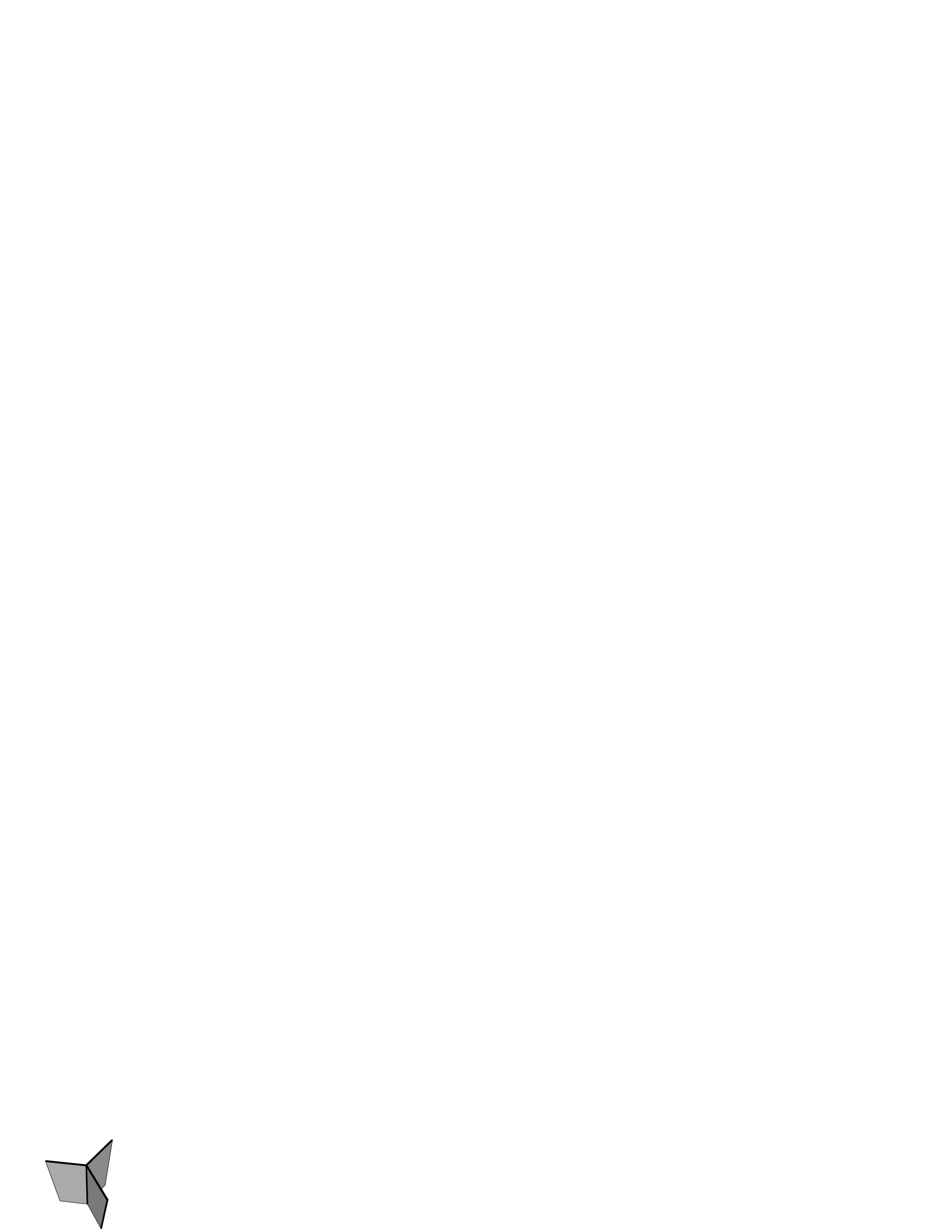
Figure 1: The conjectured optimal partition for the “sum of squares of Gaussian moments problem” described above consists of a partition of $R^{k-1}$ into $3$ parts, and the remaining $k-3$ parts are empty. This partition corresponds to a planar $120^{\circ}$ “propeller” multiplied by an orthogonal copy of $\mathbb{R}^{k-3}$.

We end this introduction with an explanation of how our work relates to the recent result of Raghavendra [19] which shows that for any generalized constraint satisfaction problem (CSP) there is a generic way of writing a semidefinate relaxation that achieves an optimal approximation ratio assuming the Unique Games Conjecture. Our clustering problem fits in the framework of [19] as follows: we wish to compute

$$\max\left\{\sum_{i,j=1}^{n}a_{ij}b_{\sigma(i)\sigma(j)}:\ \sigma:\{1,\ldots,n\}\to\{1,\ldots,k\}\right\},$$ (10)

where $(a_{ij})$ is a centered positive semi-definite matrix and $(b_{ij})$ is a positive semi-definite matrix. One can think of this problem as a CSP (with an extra global constraint corresponding to the positive semi-definiteness) where the set of variables is $\{1,\ldots,n\}$ and we wish to assign each variable a value from the domain $\{1,\ldots,k\}$. For every pair $(i,j)\in\{1,\ldots,n\}\times\{1,\ldots,n\}$, there is a constraint with weight $a_{ij}$. We get a payoff of $b_{st}$ if variables $i$ and $j$ are assigned $s\in\{1,\ldots,k\}$ and $t\in\{1,\ldots,k\}$ respectively.

Raghavendra shows that every integrality gap instance for his generic SDP relaxation can be translated into a UGC-hardness of approximation result with the hardness factor (essentially) the same as the integrality gap. We make here the non-trivial observation that in the reduction of [19], starting with an integrality gap instance for (the generic SDP relaxation of) the clustering problem (10), the matrix of the constraint weights $(a_{ij})$ indeed turns out to be positive semi-definite as required in the kernel clustering problem (this requires proof—the details are omitted since this is a digression from the topic of this paper). Thus Raghavendra’s result can be made to apply to the kernel clustering problem (i.e. the generic SDP achieves the optimum approximation ratio assuming UGC).

Nevertheless, it is also useful to look at different relaxations and rounding procedures for the following reasons. Firstly, for a given problem there could be an SDP relaxation that is more natural than the generic one and might be easier to work with. Secondly, Raghavendra’s result (that the integrality gap is same as the hardness factor) applies only when the integrality gap is a constant. This is a priori not clear for the kernel clustering problem. For instance, a priori the integrality gap could be $\Omega(\log n)$ (as is the case for Grothendieck problem on a general graph—see [1]). So before applying the result of [19], one would need to show that the integrality gap of the generic SDP is indeed a constant. Thirdly, for CSPs with negative payoffs (as is the case in the kernel clustering problem), Raghavendra shows that the value computed by the generic SDP achieves the optimal approximation ratio (modulo UGC), but the paper does not give a rounding procedure. Finally, Raghavendra’s result does not really shed light on the exact hardness threshold in the sense that it shows how to translate integrality gap instances into a UGC hardness result, but gives no idea as to how to construct an integrality gap instance in the first place. Constructing the integrality gap instance in general amounts to answering certain isoperimetric type geometric question (naturally leading to a dictatorship test, or the other way round. In other words, the geometric question itself might be inspired by the dictatorship test that we have in mind). Thus as far as we know, we cannot avoid designing an explicit dictatorship test and answering an isoperimetric type question, whether or not we start with Raghavendra’s generic SDP that is guaranteed to be optimal. As mentioned before, in the clustering problem where $B=(b_{st})$ is centered and spherical, we show that the UGC-hardness threshold is at least $\frac{1-1/k}{C(k)}$ and characterizing $C(k)$ seems to be a challenging geometric question.

2 Constant factor approximation algorithms for kernel clustering

Let $A\in M_{n}(\mathbb{R})$ and $B\in M_{k}(\mathbb{R})$ be positive semidefinite matrices. Then there are $u_{1},\ldots,u_{n}\in\mathbb{R}^{n}$ and $v_{1},\ldots,v_{k}\in\mathbb{R}^{k}$ such that $a_{ij}=\langle u_{i},u_{j}\rangle$ and $b_{ij}=\langle v_{i},v_{j}\rangle$. Such vectors can be found in polynomial time (this is simply the Cholesky decomposition). The instance of the kernel clustering problem will be called centered if $\sum_{i,j=1}^{n}a_{ij}=0$, or equivalently $\sum_{i=1}^{n}u_{i}=0$. The instance will be called spherical if $b_{ii}=1=\|v_{i}\|_{2}^{2}$ for all $i\in\{1,\ldots,k\}$. Let $R(B)$ be the radius of the smallest Euclidean ball containing $\{v_{1},\ldots,v_{k}\}$. Note that $R(B)$ is indeed only a function of $B$, i.e. it does not depend on the particular representation of $B$ as a Gram matrix. Moreover, it is possible to compute $R(B)$, and given the decomposition $b_{ij}=\langle v_{i},v_{j}\rangle$ a vector $w\in\mathbb{R}^{k}$ such that $\max_{j\in\{1,\ldots,k\}}\|v_{j}-w\|_{2}=R(B)$, in polynomial time (see [10]).

Our goal is to compute in polynomial time the quantity:

$$\mathrm{\bf Clust}(A|B)\coloneqq\max_{\sigma:\{1,\ldots,n\}\to\{1,\ldots,k\}}\sum_{i,j=1}^{n}a_{ij}b_{\sigma(i)\sigma(j)}=\max_{\sigma:\{1,\ldots,n\}\to\{1,\ldots,k\}}\sum_{i,j=1}^{n}\langle u_{i},u_{j}\rangle\langle v_{\sigma(i)},v_{\sigma(j)}\rangle.$$

Our algorithm, which is based on semidefinite programming, proceeds via the following steps:

1. Compute a Cholesky decomposition of $B$, i.e. $v_{1},\ldots,v_{k}\in\mathbb{R}^{k}$ with $b_{ij}=\langle v_{i},v_{j}\rangle$.

2. Compute (using for example [10]) $R(B)$ and a vector $w\in\mathbb{R}^{k}$ such that

   $$\max_{j\in\{1,\ldots,k\}}\|v_{j}-w\|_{2}=R(B).$$

3. Solve the semidefinite program

   $$\!\!\!\!\!\max\left\{\sum_{i,j=1}^{n}a_{ij}\cdot\left\langle\|w\|_{2}u+R(B)x_{i},\ \|w\|_{2}u+R(B)x_{j}\right\rangle:\ u,x_{1},\ldots,x_{n}\in\mathbb{R}^{n+1}\ \wedge\ \|u\|_{2}=1\ \wedge\ \forall i\ \|x_{i}\|_{2}\leq 1\right\}.$$

4. Choose $p,q\in\{1,\ldots,k\}$ such that $\|v_{p}-v_{q}\|_{2}=\max_{i,j\in\{1,\ldots,k\}}\|v_{i}-v_{j}\|_{2}$. Let $g_{1},g_{2}\in\mathbb{R}^{n+1}$ be i.i.d. standard Gaussian vectors and define $\sigma:\{1,\ldots,n\}\to\{1,\ldots,k\}$ by

   $$\sigma(r)=\left\{\begin{array}[]{ll}p&\mathrm{if}\ \langle g_{1},x_{r}\rangle\geq\langle g_{2},x_{r}\rangle,\\ q&\mathrm{if}\ \langle g_{2},x_{r}\rangle\geq\langle g_{1},x_{r}\rangle.\end{array}\right.$$ (13)

5. Choose distinct $\alpha,\beta,\gamma\in\{1,\ldots,k\}$ such that

   $$\left\|v_{\alpha}-\frac{v_{\alpha}+v_{\beta}+v_{\gamma}}{3}\right\|_{2}^{2}+\left\|v_{\beta}-\frac{v_{\alpha}+v_{\beta}+v_{\gamma}}{3}\right\|_{2}^{2}+\left\|v_{\gamma}-\frac{v_{\alpha}+v_{\beta}+v_{\gamma}}{3}\right\|_{2}^{2}$$

   is maximized among all such choices of $\alpha,\beta,\gamma$. Let $g_{1},g_{2},g_{3}\in\mathbb{R}^{n+1}$ be i.i.d. standard Gaussian vectors and define $\tau:\{1,\ldots,n\}\to\{1,\ldots,k\}$ by

   $$\tau(r)=\left\{\begin{array}[]{ll}\alpha&\mathrm{if}\ \langle g_{1},x_{r}\rangle\geq\max\left\{\langle g_{2},x_{r}\rangle,\langle g_{3},x_{r}\rangle\right\},\\ \beta&\mathrm{if}\ \langle g_{2},x_{r}\rangle\geq\max\left\{\langle g_{1},x_{r}\rangle,\langle g_{3},x_{r}\rangle\right\},\\ \gamma&\mathrm{if}\ \langle g_{3},x_{r}\rangle\geq\max\left\{\langle g_{1},x_{r}\rangle,\langle g_{2},x_{r}\rangle\right\}.\end{array}\right.$$ (17)

6. Output $\sigma$ if $\sum_{i,j=1}^{n}a_{ij}b_{\sigma(i)\sigma(j)}\geq\sum_{i,j=1}^{n}a_{ij}b_{\tau(i)\tau(j)}$. Otherwise output $\tau$.

Remark 2.1.

The astute reader might notice that there is an obvious generalization of the above algorithm. Namely for every fixed integer $s\in[2,k]$ we can choose a subset $S\subseteq\{1,..,k\}$ of cardinality $s$ which maximizes the quantity

$$\sum_{i\in S}\left\|v_{i}-\frac{1}{s}\sum_{j\in S}v_{j}\right\|_{2}^{2}.$$

Then, we can choose $s$ i.i.d. standard Gaussians $\{g_{i}\}_{i\in S}\subseteq\mathbb{R}^{n+1}$ and define $\sigma_{s}:\{1,\ldots,n\}\to\{1,\ldots,k\}$ analogously to the above, namely $\sigma_{s}(r)=i$ if

$$\langle g_{i},x_{r}\rangle=\max_{j\in S}\langle g_{j},x_{r}\rangle.$$

Then, we can consider the assignments $\sigma_{2},\sigma_{3},\ldots,\sigma_{s}$ and choose the one which maximizes the objective $\sum_{i,j=1}^{n}a_{ij}b_{\sigma_{\ell}(i)\sigma_{\ell}(j)}$. In spite of this flexibility, it turns out that the the rounding method described above does not improve if we take $s\geq 4$. In order to demonstrate this fact we will proceed below to analyze the algorithm for general $s$, and then optimize over $s$.

Bounds on the performance of the above algorithm are contained in the following theorem:

Theorem 2.1.

Assume that $A$ is centered, i.e. that $\sum_{i,j=1}^{n}a_{ij}=0$. Let $p,q,\alpha,\beta,\gamma\in\{1,\ldots,k\}$ and $v_{1},\ldots,v_{k}$ be as in the description above. Then the algorithm outputs in polynomial time a random assignment $\lambda:\{1,\ldots,n\}\to\{1,\ldots,k\}$ satisfying

$$\mathrm{\bf Clust}(A|B)\\ \leq\min\left\{\frac{2\pi R(B)^{2}}{\|v_{p}-v_{q}\|_{2}^{2}},\frac{16\pi R(B)^{2}}{9\left(\left\|v_{\alpha}-\frac{v_{\alpha}+v_{\beta}+v_{\gamma}}{3}\right\|_{2}^{2}+\left\|v_{\beta}-\frac{v_{\alpha}+v_{\beta}+v_{\gamma}}{3}\right\|_{2}^{2}+\left\|v_{\gamma}-\frac{v_{\alpha}+v_{\beta}+v_{\gamma}}{3}\right\|_{2}^{2}\right)}\right\}\mathbb{E}\left[\sum_{i,j=1}^{n}a_{ij}b_{\lambda(i)\lambda(j)}\right].$$ (18)

In particular we always have

$$\mathrm{\bf Clust}(A|B)\leq\pi\left(1-\frac{1}{k}\right)\mathbb{E}\left[\sum_{i,j=1}^{n}a_{ij}b_{\lambda(i)\lambda(j)}\right],$$ (19)

and if $B$ is centered and spherical, i.e. $\sum_{i,j=1}^{k}b_{ij}=0$ and $b_{ii}=1$ for all $i$, then

$$\mathrm{\bf Clust}(A|B)\leq\frac{8\pi}{9}\left(1-\frac{1}{k}\right)\mathbb{E}\left[\sum_{i,j=1}^{n}a_{ij}b_{\lambda(i)\lambda(j)}\right].$$ (20)

The same bound in (20) holds true if $B$ is the identity matrix.

We single out in the next theorem the case $k\in\{2,3\}$, since in these cases we have matching UGC hardness results. Note that for general $k$ we obtain a factor $\pi$ approximation algorithm, answering positively the question posed by Song, Smola, Gretton and Borgwardt in [23].

Theorem 2.2.

Assume that $A$ is centered and $B$ is a $2\times 2$ matrix. Then our algorithm achieves a $\frac{\pi}{2}$ approximation factor. Assuming the Unique Games Conjecture no polynomial time algorithm achieves an approximation guarantee smaller than $\frac{\pi}{2}$ in this case.

Assume that $A$ is centered, $k=3$ and $B$ is centered and spherical (since $k=3$ this forces $B$ to be the Gram matrix of the-degree three roots of unity in the complex plane). Then our algorithm achieves an approximation factor of $\frac{16\pi}{27}$. Assuming the Unique Games Conjecture no polynomial time algorithm achieves an approximation guarantee smaller than $\frac{16\pi}{27}$ in this case.

In fact, we believe that the UGC hardness threshold for the kernel clustering problem when $A$ is centered and $B$ is spherical and centered is exactly

$$\frac{8\pi}{9}\left(1-\frac{1}{k}\right).$$

In Section 3 we describe a geometric conjecture which we show implies this tight UGC threshold for general $k$.

We end the discussion by stating a (probably suboptimal) constant factor approximation result when $A$ is not necessarily centered (note that this case is of lesser interest in terms of the applications in machine learning). In this case the above algorithm gives a constant factor approximation. The slightly better bound on the approximation factor in Theorem 2.3 below follows from a variant of the above algorithm which will be described in its proof.

Theorem 2.3.

For general $A$ and $B$ (not necessarily centered) there exists a polynomial time algorithm that achieves an approximation factor of

$$1+\frac{2\pi}{\|v_{p}-v_{q}\|_{2}^{2}}\cdot\max_{i\in\{1,\ldots,k\}}\left\|v_{i}-\frac{v_{p}+v_{q}}{2}\right\|_{2}^{2}\leq 1+\frac{3\pi}{2}.$$

The proof of Theorem 2.2 is contained in Section 3. We shall now proceed to prove Theorem 2.1. Before doing so we will show how the general bound in (18) implies the bounds (19) and (20). The proof of Theorem 2.3 is deferred to the end of this section.

To prove that (18) implies (19) let $D$ denote the diameter of the set $\{v_{1},\ldots,v_{k}\}$, i.e. $D=\|v_{p}-v_{q}\|_{2}$. A classical theorem of Jung [12] (see [7]) says that

$$R(B)\leq D\cdot\sqrt{\frac{k-1}{2k}},$$

and (19) follows immediately by taking the first term in the minimum in (18).

We shall now show that (18) implies (20) when $B$ is either centered and spherical or the identity matrix. Assume first of all that $B$ is centered and spherical. Note that since $v_{1},\ldots,v_{k}$ are unit vectors, $R(B)\leq 1$. Hence, by considering the second term in the minimum in (18) we see that it is enough to show that there exist $\alpha,\beta,\gamma\in\{1,\ldots,k\}$ for which

$$\left\|v_{\alpha}-\frac{v_{\alpha}+v_{\beta}+v_{\gamma}}{3}\right\|_{2}^{2}+\left\|v_{\beta}-\frac{v_{\alpha}+v_{\beta}+v_{\gamma}}{3}\right\|_{2}^{2}+\left\|v_{\gamma}-\frac{v_{\alpha}+v_{\beta}+v_{\gamma}}{3}\right\|_{2}^{2}\geq\frac{2k}{k-1}.$$

This follows from an averaging argument. Indeed,

$$\frac{1}{\binom{k}{3}}\sum_{\begin{subarray}{c}\alpha,\beta,\gamma\in\{1,\ldots,k\}\\ \alpha<\beta<\gamma\end{subarray}}\left(\left\|v_{\alpha}-\frac{v_{\alpha}+v_{\beta}+v_{\gamma}}{3}\right\|_{2}^{2}+\left\|v_{\beta}-\frac{v_{\alpha}+v_{\beta}+v_{\gamma}}{3}\right\|_{2}^{2}+\left\|v_{\gamma}-\frac{v_{\alpha}+v_{\beta}+v_{\gamma}}{3}\right\|_{2}^{2}\right)\\ =\frac{2}{k}\sum_{i=1}^{k}\|v_{i}\|_{2}^{2}-\frac{2}{k(k-1)}\sum_{\begin{subarray}{c}i,j\in\{1,\ldots,k\}\\ i\neq j\end{subarray}}\langle v_{i},v_{j}\rangle=\frac{2}{k}\sum_{i=1}^{k}b_{ii}-\frac{2}{k(k-1)}\left(\sum_{i,j=1}^{k}b_{ij}-\sum_{i=1}^{k}b_{ii}\right)=\frac{2k}{k-1}.$$

This complete the proof of (20) when $B$ is spherical and centered. The same bound holds true when $B=I_{k}$ is the identity matrix since in this case if we denote by $e_{1},\ldots,e_{k}$ the standard unit basis of $\mathbb{R}^{k}$ and $e=\frac{1}{k}\sum_{i=1}^{k}e_{i}$ then for every assignment $\lambda:\{1,\ldots,n\}\to\{1,\ldots,k\}$ we have

$$\sum_{i,j=1}^{n}a_{ij}(I_{k})_{\lambda(i)\lambda(j)}=\sum_{i,j=1}^{n}\langle u_{i},u_{j}\rangle\langle e_{\lambda(i)},e_{\lambda(j)}\rangle\\ =\sum_{i,j=1}^{n}\langle u_{i},u_{j}\rangle\langle e_{\lambda(i)}-e,e_{\lambda(j)}-e\rangle+2\left\langle\sum_{i=1}^{n}u_{i},\sum_{j=1}^{n}\langle e,e_{\lambda(j)}\rangle u_{j}\right\rangle-\|e\|_{2}^{2}\left\|\sum_{i=1}^{k}u_{i}\right\|_{2}^{2}.$$ (21)

The last two terms in (21) vanish since $A$ is centered. Thus

$$\sum_{i,j=1}^{n}a_{ij}(I_{k})_{\lambda(i)\lambda(j)}=\frac{k-1}{k}\sum_{i,j=1}^{n}a_{ij}c_{\lambda(i)\lambda(j)},$$

where $C=(c_{ij})=\frac{k}{k-1}(\langle e_{i}-e,e_{j}-e\rangle)$ is spherical and centered. Thus the case of the identity matrix reduces to the previous analysis.

Proof of Theorem 2.1.

Denote

$$\mathrm{SDP}\coloneqq\max\sum_{i,j=1}^{n}a_{ij}\cdot\left\langle\|w\|_{2}u+R(B)x_{i},\ \|w\|_{2}u+R(B)x_{j}\right\rangle,$$

where the maximum is taken over all $u,x_{1},\ldots,x_{n}\in\mathbb{R}^{n+1}$ such that $\|u\|_{2}=1$ and $\|x_{i}\|_{2}\leq 1$ for all $i$. Observe that

$$\mathrm{SDP}\geq\mathrm{\bf Clust}(A|B).$$ (22)

Indeed, for every $\lambda:\{1,\ldots,n\}\to\{1,\ldots,k\}$ define $u=\frac{w}{\|w\|_{2}}$ and $x_{i}=\frac{v_{\lambda(i)}-w}{R(B)}$ and note that in this case

$$\sum_{i,j=1}^{n}a_{ij}\cdot\left\langle\|w\|_{2}u+R(B)x_{i},\ \|w\|_{2}u+R(B)x_{j}\right\rangle=\sum_{i,j=1}^{n}a_{ij}b_{\lambda(i)\lambda(j)}.$$

Let $u^{*},x_{1}^{*},\ldots,x_{n}^{*}$ be the optimal solution to the SDP. It will be convenient to think of the SDP solution as being split into two parts. So we rewrite

$${\rm SDP} = \sum_{i,j=1}^{n}a_{ij}\cdot\left\langle\|w\|_{2}u^{*}+R(B)x_{i}^{*},\ \|w\|_{2}u^{*}+R(B)x_{j}^{*}\right\rangle$$

$$= \sum_{i,j=1}^{n}\langle u_{i},u_{j}\rangle\cdot\langle\|w\|_{2}u^{*}+R(B)x^{*}_{i},\ \|w\|_{2}u^{*}+R(B)x_{j}^{*}\rangle$$

$$= \left\|\sum_{i=1}^{n}u_{i}\otimes(\|w\|_{2}u^{*}+R(B)x_{i}^{*})\right\|_{2}^{2}$$

$$= \left\|\left(\|w\|_{2}\left(\sum_{i=1}^{n}u_{i}\right)\otimes u^{*}\right)\ +\ \left(R(B)\sum_{i=1}^{n}u_{i}\otimes x_{i}^{*}\right)\right\|_{2}^{2}$$

$$= \|P+Q\|_{2}^{2},$$ (24)

where

$$P\coloneqq\|w\|_{2}\sum_{i=1}^{n}u_{i}\otimes u^{*},$$ (25)

and

$$Q\coloneqq R(B)\sum_{i=1}^{n}u_{i}\otimes x_{i}^{*}.$$ (26)

Observe in passing that (2) implies that the objective function of the SDP is convex as a function of $u,x_{1},\ldots,x_{n}$, and therefore we may assume that $\|u^{*}\|_{2}=1$ and $\|x_{i}^{*}\|_{2}=1$ for all $i$.

We shall now proceed with the analysis of our algorithm while using the variant described in Remark 2.1. This will not create any additional complication, and will allow us to explain why there is no advantage in working with subsets of size $s\geq 4$. Recall the setting: for a fixed integer $s\in[2,k]$ we choose a subset $S\subseteq\{1,..,k\}$ of cardinality $s$ which maximizes the quantity

$$\sum_{i\in S}\left\|v_{i}-\frac{1}{s}\sum_{j\in S}v_{j}\right\|_{2}^{2}.$$

Then, we choose $s$ i.i.d. standard Gaussians $\{g_{i}\}_{i\in S}\subseteq\mathbb{R}^{n+1}$ and define $\sigma:\{1,\ldots,n\}\to\{1,\ldots,k\}$ by setting $\sigma(r)=i$ if

$$\langle g_{i},x_{r}^{*}\rangle=\max_{j\in S}\langle g_{j},x_{r}^{*}\rangle.$$

Fix $i,j\in\{1,\ldots,n\}$. As proved by Frieze and Jerrum in [9] (see Lemma 5 there), we have:

$$\Pr\left[\sigma(i)=\sigma(j)\right]=\sum_{m=0}^{\infty}R_{m}(s)\langle x_{i}^{*},x_{j}^{*}\rangle^{m},$$

where the power series converges on $[-1,1]$ and all the coefficients $R_{m}(s)$ are non-negative. Moreover $R_{0}(s)=\frac{1}{s}$ and

$$R_{1}(s)=\frac{1}{s-1}\left({\mathbb{E}}\left[\max_{j\in S}g_{j}\right]\right)^{2}=\frac{s}{(2\pi)^{s/2}}\int_{-\infty}^{\infty}xe^{-x^{2}/2}\left(\int_{-\infty}^{x}e^{-y^{2}/2}dy\right)^{s-1}dx.$$

Note that conditioned on the event $\sigma(i)=\sigma(j)$, the random index $\sigma(i)$ is uniformly distributed over $S$. Also, conditioned on the event $\sigma(i)\neq\sigma(j)$, the pair $(\sigma(i),\sigma(j))$ is uniformly distributed over all $s(s-1)$ pairs of distinct indices in $S$. Thus

$$\mathbb{E}[b_{\sigma(i)\sigma(j)}]={\rm Pr}[\sigma(i)=\sigma(j)]\cdot\left(\frac{1}{s}\sum_{\ell\in S}b_{\ell\ell}\right)+{\rm Pr}[\sigma(i)\not=\sigma(j)]\cdot\left(\frac{1}{s(s-1)}\sum_{\begin{subarray}{c}\ell,t\in S\\ \ell\neq t\end{subarray}}b_{\ell t}\right).$$

Denote $\Phi=\frac{1}{s}\sum_{\ell\in S}b_{\ell\ell}$ and $\Psi=\frac{1}{s(s-1)}\sum_{\begin{subarray}{c}\ell,t\in S\\ \ell\neq t\end{subarray}}b_{\ell t}$. (note that $\Phi,\Psi$ depend on the matrix $B$ as well as the choice of the subset $S\subseteq\{1,\ldots,k\}$. Thus

$$\mathbb{E}[b_{\sigma(i)\sigma(j)}]=\left(\sum_{m=0}^{\infty}R_{m}(s)\langle x_{i}^{*},x_{j}^{*}\rangle^{m}\right)\cdot\Phi\ +\ \left(1-\sum_{m=0}^{\infty}R_{m}(s)\langle x_{i}^{*},x_{j}^{*}\rangle^{m}\right)\cdot\Psi\\ =\left(\Psi+(\Phi-\Psi)R_{0}(s)\right)+(\Phi-\Psi)\sum_{m=1}^{\infty}R_{m}(s)\langle x_{i}^{*},x_{j}^{*}\rangle^{m}.$$ (27)

Write $v\coloneqq\frac{1}{s}\sum_{\ell\in S}v_{\ell}$. Observe that

$$\Psi+(\Phi-\Psi)R_{0}(s)=\|v\|_{2}^{2}.$$ (28)

Indeed, since $R_{0}(s)=1/s$ we have

$$\Psi+(\Phi-\Psi)R_{0}(s)=\left(1-\frac{1}{s}\right)\left(\frac{1}{s(s-1)}\sum_{\begin{subarray}{c}\ell,t\in S\\ \ell\neq t\end{subarray}}b_{\ell t}\right)+\frac{1}{s}\left(\frac{1}{s}\sum_{\ell\in S}b_{\ell\ell}\right)=\frac{1}{s^{2}}\sum_{\ell,t\in S}b_{\ell t}=\left\|\frac{1}{s}\sum_{\ell\in S}^{s}v_{\ell}\right\|_{2}^{2}=\|v\|_{2}^{2}.$$

Moreover,

$$(s-1)(\Phi-\Psi)=\sum_{\ell\in S}\|v_{\ell}-v\|_{2}^{2}.$$ (29)

In particular $\Phi-\Psi\geq 0$. To prove (29) we simply expand:

$$\sum_{\ell\in S}\|v_{\ell}-v\|_{2}^{2}=\sum_{\ell\in S}\|v_{\ell}\|_{2}^{2}-s\|v\|_{2}^{2}=s\Phi-\frac{1}{s}\sum_{\ell,t\in S}b_{\ell t}=s\Phi-\frac{1}{s}\left(s\Phi+s(s-1)\Psi\right)=(s-1)(\Phi-\Psi).$$

Multiplying both sides of equation (27) by $a_{ij}$ and summing over $i,j\in\{1,\ldots,n\}$ while using (28) we get that

$$\mathbb{E}\left[\sum_{i,j=1}^{n}a_{ij}b_{\sigma(i)\sigma(j)}\right]=\|v\|_{2}^{2}\sum_{i,j=1}^{n}a_{ij}+(\Phi-\Psi)R_{1}(s)\sum_{i,j=1}^{n}a_{ij}\langle x_{i}^{*},x_{j}^{*}\rangle+(\Phi-\Psi)\sum_{m=2}^{\infty}R_{m}(s)\sum_{i,j=1}^{n}a_{ij}\langle x_{i}^{*},x_{j}^{*}\rangle^{m}.$$ (30)

Note that for every $m\geq 1$ we have

$$\sum_{i,j=1}^{n}a_{ij}\langle x_{i}^{*},x_{j}^{*}\rangle^{m}=\sum_{i,j=1}^{n}\langle u_{i},u_{j}\rangle\left\langle(x_{i}^{*})^{\otimes m},(x_{j}^{*})^{\otimes m}\right\rangle=\left\|\sum_{i=1}^{n}u_{i}\otimes(x_{i}^{*})^{\otimes m}\right\|_{2}^{2}\geq 0.$$ (31)

Plugging (31) into (30), and using the fact that $\Phi-\Psi\geq 0$ and the positivity of $\mathbb{R}_{m}(s)$, we conclude that

$$\mathbb{E}\left[\sum_{i,j=1}^{n}a_{ij}b_{\sigma(i)\sigma(j)}\right]\geq\|v\|_{2}^{2}\sum_{i,j=1}^{n}a_{ij}+(\Phi-\Psi)R_{1}(s)\sum_{i,j=1}^{n}a_{ij}\langle x_{i}^{*},x_{j}^{*}\rangle.$$ (32)

We shall now use the fact that $\sum_{i,j=1}^{n}a_{ij}=0$ for the first time. In this case $P=0$ (see equations (24) and (25)) so that

$$\mathrm{SDP}=R(B)^{2}\sum_{i,j=1}^{n}a_{ij}\langle x_{i}^{*},x_{j}^{*}\rangle.$$ (33)

Hence, using (32) and (28) we get the bound

$$\mathbb{E}\left[\sum_{i,j=1}^{n}a_{ij}b_{\sigma(i)\sigma(j)}\right]\geq\frac{R_{1}(s)\sum_{\ell\in S}\|v_{\ell}-v\|_{2}^{2}}{(s-1)R(B)^{2}}\cdot\mathrm{SDP}\stackrel{{\scriptstyle\eqref{eq:is relaxtion}}}{{\geq}}\frac{R_{1}(s)\sum_{\ell\in S}\|v_{\ell}-v\|_{2}^{2}}{(s-1)R(B)^{2}}\cdot\mathrm{\bf Clust}(A|B).$$ (34)

The term $R_{1}(s)$ is studied in Section 3.1, where its geometric interpretation is explained. In particular, it follows from Corollary 3.6 and Corollary 3.4 that $R_{1}(s)<R_{1}(3)$ for every $s\geq 4$ and that $R_{1}(2)=\frac{1}{\pi}$ and $R_{1}(3)=\frac{9}{8\pi}$. Hence the cases $s\in\{2,3\}$ in (34) conclude the proof of Theorem 2.1. Moreover, we see that for $s\geq 4$ the lower bound in (34) is worse than the lower bound obtained when case $s=3$. Indeed, we have already noted that in this case $R_{1}(s)<R_{1}(3)$. In addition,

$$\frac{1}{\binom{s}{3}}\sum_{\begin{subarray}{c}T\subseteq S\\ |T|=3\end{subarray}}\frac{1}{2}\sum_{\ell\in T}\left\|v_{\ell}-\frac{1}{3}\sum_{t\in T}v_{t}\right\|_{2}^{2}=\frac{1}{s}\sum_{\ell\in S}\|v_{\ell}\|_{2}^{2}-\frac{1}{s(s-1)}\sum_{\begin{subarray}{c}\ell,t\in S\\ \ell\neq t\end{subarray}}\langle v_{\ell},v_{t}\rangle=\frac{1}{s-1}\sum_{\ell\in S}\left\|v_{\ell}-\frac{1}{s}\sum_{t\in S}v_{t}\right\|_{2}^{2}.$$

This implies that there exists $T\subseteq S$ with $|T|=3$ for which

$$\frac{1}{2}\sum_{\ell\in T}\left\|v_{\ell}-\frac{1}{3}\sum_{t\in T}v_{t}\right\|_{2}^{2}\geq\frac{1}{s-1}\sum_{\ell\in S}\|v_{\ell}-v\|_{2}^{2},$$

so that when $s\geq 4$ the lower bound in (34) is inferior to the same lower bound when $s=3$. ∎

It remains to deal with the case $\sum_{i,j=1}^{n}a_{ij}>0$, i.e. to prove Theorem 2.3.

Proof of Theorem 2.3.

We slightly modify the algorithm that was studied in Theorem 2.1. Let $v_{1},\ldots,v_{k}$ and $p,q\in\{1,\ldots,k\}$ be as before, that is $b_{ij}=\langle v_{i},v_{j}\rangle$ and $\|v_{p}-v_{q}\|_{2}=\max_{i,j\in\{1,\ldots,k\}}\|v_{i}-v_{j}\|_{2}=D$, the diameter of the set $\{v_{1},\ldots,v_{k}\}\in\mathbb{R}^{k}$. Denote $w^{\prime}\coloneqq\frac{v_{p}+v_{q}}{2}$ and

$$R^{\prime}(B)\coloneqq\max_{i\in\{1,\ldots,k\}}\left\|v_{i}-w^{\prime}\right\|_{2}.$$

We now consider the modified semidefinite program

$$\mathrm{SDP}\coloneqq\max\sum_{i,j=1}^{n}a_{ij}\cdot\left\langle\|w^{\prime}\|_{2}u+R^{\prime}(B)x_{i},\ \|w^{\prime}\|_{2}u+R^{\prime}(B)x_{j}\right\rangle,$$

where the maximum is taken over all $u,x_{1},\ldots,x_{n}\in\mathbb{R}^{n+1}$ such that $\|u\|_{2}=1$ and $\|x_{i}\|_{2}\leq 1$ for all $i$. From now on we will use the notation of the proof of Theorem 2.1 with $w$ replaced by $w^{\prime}$ and $R(B)$ replaced by $R^{\prime}(B)$ (this slight abuse of notation will not create any confusion). As before, we let $g_{1},g_{2}\in\mathbb{R}^{n+1}$ be i.i.d. standard Gaussian vectors and define $\sigma:\{1,\ldots,n\}\to\{1,\ldots,k\}$ by

$$\sigma(r)=\left\{\begin{array}[]{ll}p&\mathrm{if}\ \langle g_{1},x_{r}\rangle\geq\langle g_{2},x_{r}\rangle,\\ q&\mathrm{if}\ \langle g_{2},x_{r}\rangle\geq\langle g_{1},x_{r}\rangle.\end{array}\right.$$ (37)

Note that the first place in the proof of Theorem 2.1 where the assumption that $A$ is centered was used in equation (33). Hence, in the present setting we still have the bounds

$$\mathrm{\bf Clust}(A|B)\leq\mathrm{SDP}=\|P+Q\|_{2}^{2}\leq\left(\|P\|_{2}+\|Q\|_{2}\right)^{2},$$ (38)

where $P$ and $Q$ are defined in (25) and (26) (with $w$ and $R(B)$ replaced by $w^{\prime}$ and $R^{\prime}(B)$, respectively). Also, it follows from (32) that

$$\mathbb{E}\left[\sum_{i,j=1}^{n}a_{ij}b_{\sigma(i)\sigma(j)}\right]\geq\|v\|_{2}^{2}\sum_{i,j=1}^{n}a_{ij}+\left(\|v_{p}-v\|_{2}^{2}+\|v_{q}-v\|_{2}^{2}\right)R_{1}(2)\sum_{i,j=1}^{n}a_{ij}\langle x_{i}^{*},x_{j}^{*}\rangle,$$ (39)

where $v=\frac{v_{p}+v_{q}}{2}=w^{\prime}$. Note that $\|v_{p}-v\|_{2}^{2}+\|v_{q}-v\|_{2}^{2}=\frac{D^{2}}{2}$, and recall that $R_{1}(2)=\frac{1}{\pi}$. Thus (39) becomes:

$$\mathbb{E}\left[\sum_{i,j=1}^{n}a_{ij}b_{\sigma(i)\sigma(j)}\right]\geq\|w^{\prime}\|_{2}^{2}\sum_{i,j=1}^{n}a_{ij}+\frac{D^{2}}{2\pi}\sum_{i,j=1}^{n}a_{ij}\langle x_{i}^{*},x_{j}^{*}\rangle,$$ (40)

Note that

$$\|P\|_{2}^{2}=\|w^{\prime}\|_{2}^{2}\cdot\left\|\sum_{i=1}^{n}u_{i}\otimes u^{*}\right\|_{2}^{2}=\|w^{\prime}\|_{2}^{2}\cdot\|u^{*}\|_{2}^{2}\sum_{i,j=1}^{n}\langle u_{i},u_{j}\rangle=\|w^{\prime}\|_{2}^{2}\sum_{i,j=1}^{n}a_{ij}.$$ (41)

and

$$\|Q\|_{2}^{2}=R^{\prime}(B)^{2}\cdot\left\|\sum_{i=1}^{n}u_{i}\otimes x_{i}^{*}\right\|_{2}^{2}=R^{\prime}(B)^{2}\sum_{i,j=1}^{n}a_{ij}\langle x_{i}^{*},x_{j}^{*}\rangle.$$ (42)

Combining (38) and (40) with (41) and (42) we see that

$$\mathrm{\bf Clust}(A|B)\leq\frac{\left(\|P\|_{2}+\|Q\|_{2}\right)^{2}}{\|P_{2}\|_{2}^{2}+c\|Q\|_{2}^{2}}\cdot\mathbb{E}\left[\sum_{i,j=1}^{n}a_{ij}b_{\sigma(i)\sigma(j)}\right],$$ (43)

where $c=\frac{D^{2}}{2\pi R^{\prime}(B)^{2}}$. The convexity of the function $x\to x^{2}$ implies that

$$\left(\|P\|_{2}+\|Q\|_{2}\right)^{2}=\left(\frac{c}{c+1}\cdot\frac{c+1}{c}\|P\|_{2}^{2}+\left(1-\frac{c}{c+1}\right)(c+1)\|Q\|_{2}^{2}\right)^{2}\\ \leq\frac{c+1}{c}\|P\|_{2}^{2}+(c+1)\|Q\|_{2}^{2}=\left(1+\frac{1}{c}\right)\left(\|P\|_{2}^{2}+c\|Q\|_{2}^{2}\right).$$

Thus (43) implies that our algorithm achieves an approximation guarantee bounded above by

$$1+\frac{1}{c}=1+\frac{2\pi R^{\prime}(B)^{2}}{D^{2}}=1+\frac{2\pi}{\|v_{p}-v_{q}\|_{2}^{2}}\cdot\max_{i\in\{1,\ldots,k\}}\left\|v_{i}-\frac{v_{p}+v_{q}}{2}\right\|_{2}^{2}.$$

It remains to note that for every $i\in\{1,\ldots,k\}$ we know that $\|v_{i}-v_{p}\|_{2},\|v_{i}-v_{q}\|_{2}\leq D$ and therefore $\|v_{i}-w^{\prime}\|_{2}\leq\frac{\sqrt{3}}{2}D$. This implies that our approximation guarantee is bounded from above by $1+\frac{3\pi}{2}$. ∎

3 UGC hardness

3.1 Geometric preliminaries: Propeller problems

Let $\gamma_{n}$ be the standard Gaussian measure on $\mathbb{R}^{n}$. For any integer $k\geq 2$ define

$$C(n,k)\coloneqq\sup\left\{\sum_{j=1}^{k}\left\|\int_{\mathbb{R}^{n}}xf_{j}(x)d\gamma_{n}(x)\right\|_{2}^{2}:\ f_{1},\ldots,f_{k}\in L_{2}(\gamma_{n})\ \wedge\ \forall j\ f_{j}\geq 0\ \wedge\ \sum_{j=1}^{k}f_{j}\leq 1\right\}.$$ (44)

We first observe that the supremum in (44) is attained at a $k$-tuple of functions which correspond to a partition of $\mathbb{R}^{n}$:

Lemma 3.1.

There exist disjoint measurable sets $A_{1},\ldots,A_{k}\subseteq\mathbb{R}^{n}$ such that $A_{1}\cup A_{2}\cup\cdots\cup A_{k}=\mathbb{R}^{n}$ and

$$\sum_{j=1}^{k}\left\|\int_{A_{j}}xd\gamma_{n}(x)\right\|_{2}^{2}=C(n,k).$$

Proof.

Let $H$ be the Hilbert space $L_{2}(\gamma_{n})\oplus L_{2}(\gamma_{n})\oplus\cdots\oplus L_{2}(\gamma_{n})$ ($k$ times). Define $K\subseteq H$ to be the set of all $(f_{1},\ldots,f_{k})\in H$ such that $f_{j}\geq 0$ for all $j$ and $\sum_{j=1}^{k}f_{j}\leq 1$. Then $K$ is a closed convex and bounded subset of $H$, and hence by the Banach-Alaoglu it is weakly compact. The mapping $\psi:K\to\mathbb{R}$ given by

$$\psi(f_{1},\ldots,f_{k})\coloneqq\sum_{j=1}^{k}\left\|\int_{\mathbb{R}^{n}}xf_{j}(x)d\gamma_{n}(x)\right\|_{2}^{2}=\sum_{j=1}^{k}\sum_{i=1}^{n}\left(\int_{\mathbb{R}^{n}}x_{i}f_{j}(x)d\gamma_{n}(x)\right)^{2}$$

is weakly continuous since the mapping $(x_{1},\ldots,x_{n})\to x_{j}$ is in $L_{2}(\gamma_{n})$ for each $j$. Hence $\psi$ attains its maximum on $K$, say at $(f_{1}^{*},\ldots,f_{k}^{*})\in K$.

Define $z_{j}\coloneqq\int_{\mathbb{R}^{n}}xf_{j}^{*}(x)d\gamma_{n}(x)\in\mathbb{R}^{n}$ and let

$$w\coloneqq-\sum_{j=1}^{k}z_{j}=\int_{\mathbb{R}^{n}}x\left(1-\sum_{j=1}^{k}f_{j}^{*}(x)\right)d\gamma_{n}(x).$$

Note that

$$\frac{1}{k}\sum_{i=1}^{k}\left(\sum_{\begin{subarray}{c}1\leq j\leq k\\ j\neq i\end{subarray}}\|z_{j}\|_{2}^{2}+\|z_{i}+w\|_{2}^{2}\right)=\sum_{j=1}^{k}\|z_{j}\|_{2}^{2}+\left(1-\frac{2}{k}\right)\|w\|_{2}^{2}\geq\sum_{j=1}^{k}\|z_{j}\|_{2}^{2},$$

which implies the existence of $i\in\{1,\ldots,k\}$ for which

$$\sum_{\begin{subarray}{c}1\leq j\leq k\\ j\neq i\end{subarray}}\|z_{j}\|_{2}^{2}+\|z_{i}+w\|_{2}^{2}\geq\sum_{j=1}^{k}\|z_{j}\|_{2}^{2}.$$

Hence, if we define for $j\in\{1,\ldots,k\}$,

$$g_{j}\coloneqq\left\{\begin{array}[]{ll}f_{j}^{*}&j\neq i\\ f_{i}^{*}+1-\sum_{j=1}^{k}f_{j}^{*}&j=i\end{array}\right.$$

then $(g_{1},\ldots,g_{k})\in K$, and

$$C(n,k)\geq\sum_{j=1}^{k}\left\|\int_{\mathbb{R}^{n}}xg_{j}(x)d\gamma_{n}(x)\right\|_{2}^{2}=\sum_{\begin{subarray}{c}1\leq j\leq k\\ j\neq i\end{subarray}}\|z_{j}\|_{2}^{2}+\|z_{i}+w\|_{2}^{2}\geq\sum_{j=1}^{n}\|z_{j}\|_{2}^{2}=C(n,k).$$

So

$$\sum_{j=1}^{k}\left\|\int_{\mathbb{R}^{n}}xg_{j}(x)d\gamma_{n}(x)\right\|_{2}^{2}=C(n,k).$$

Note that $\sum_{j=1}^{k}g_{j}=1$, so we can define a random partition $A_{1},\ldots,A_{k}$ of $\mathbb{R}^{n}$ as follows: let $\{s_{x}\}_{x\in\mathbb{R}^{n}}$ be independent random variables taking values in $\{1,\ldots,k\}$ such that $\Pr(s_{x}=j)=g_{j}(x)$, and define $A_{j}\coloneqq\{x\in\mathbb{R}^{n}:\ s_{x}=j\}$. Then by convexity and the definition of $C(n,k)$ we see that

$$\mathbb{E}\sum_{j=1}^{k}\left\|\int_{A_{j}}xd\gamma_{n}(x)\right\|_{2}^{2}\geq\sum_{j=1}^{k}\left\|\int_{\mathbb{R}^{n}}\big{(}\mathbb{E}\mathbf{1}_{A_{j}}(x)\big{)}xd\gamma_{n}(x)\right\|_{2}^{2}=\sum_{j=1}^{k}\left\|\int_{\mathbb{R}^{n}}xg_{j}(x)d\gamma_{n}(x)\right\|_{2}^{2}=C(n,k).$$

It therefore follows that there exists a partition as required. ∎

Lemma 3.2.

If $n\geq k-1$ then $C(n,k)=C(k-1,k)$ and if $n<k-1$ then $C(n,k)=C(n,n+1)$.

Proof.

Assume first of all that $n\geq k-1$. The inequality $C(n,k)\geq C(k-1,k)$ is easy since for every $f_{1},\ldots,f_{k}\in L_{2}(\gamma_{k-1})$ which satisfy $f_{j}\geq 0$ for all $j\in\{1,\ldots,k\}$ and $f_{1}+\cdots+f_{k}\leq 1$ we can define $\widetilde{f}_{1},\ldots\widetilde{f}_{k}:\mathbb{R}^{n}=\mathbb{R}^{k-1}\times\mathbb{R}^{n-k+1}\to\mathbb{R}$ by $\widetilde{f}_{j}(x,y)=f_{j}(x)$. Then $\widetilde{f}_{1},\ldots\widetilde{f}_{k}\in L_{2}(\gamma_{n})$, $\widetilde{f}_{1},\ldots\widetilde{f}_{k}\geq 0$, $\widetilde{f}_{1}+\cdots+\widetilde{f}_{k}\leq 1$ and $\sum_{j=1}^{k}\left\|\int_{\mathbb{R}^{k-1}}xf_{j}(x)d\gamma_{k-1}(x)\right\|_{2}^{2}=\sum_{j=1}^{k}\left\|\int_{\mathbb{R}^{n}}x\widetilde{f}_{j}(x)d\gamma_{n}(x)\right\|_{2}^{2}$. In the reverse direction, by Lemma 3.1 there is a measurable partition $A_{1},\ldots,A_{k}$ of $\mathbb{R}^{n}$ such that if we define $z_{j}\coloneqq\int_{A_{j}}xd\gamma_{n}(x)\in\mathbb{R}^{n}$ then we have $\sum_{j=1}^{k}\left\|z_{j}\right\|_{2}^{2}=C(n,k)$. Note that

$$\sum_{j=1}^{k}z_{j}=\int_{\mathbb{R}^{n}}\left(\sum_{j=1}^{k}\mathbf{1}_{A_{j}}\right)xd\gamma_{n}(x)=\int_{\mathbb{R}^{n}}xd\gamma_{n}(x)=0.$$

Hence the dimension of the subspace $V\coloneqq\mathrm{span}\{z_{1},\ldots,z_{k}\}$ is $d\leq k-1$. Define $g_{1},\ldots,g_{k}:V\to[0,1]$ by

$$g_{j}(x)=\gamma_{V^{\perp}}\left((A_{j}-x)\cap V^{\perp}\right).$$

Then $g_{1}+\cdots+g_{k}=1$, so that

$$C(k-1,k)\geq C(d,k)\geq\sum_{j=1}^{k}\left\|\int_{V}xg_{j}(x)d\gamma_{V}(x)\right\|_{2}^{2}=\sum_{j=1}^{k}\left\|\int_{V}\int_{V^{\perp}}\mathbf{1}_{A_{j}}(x+y)xd\gamma_{V}(x)d\gamma_{V^{\perp}}(y)\right\|_{2}^{2}\\ =\sum_{j=1}^{k}\left\|\int_{A_{j}}\mathrm{Proj}_{V}(w)d\gamma_{n}(w)\right\|_{2}^{2}=\sum_{j=1}^{k}\left\|\mathrm{Proj}_{V}(z_{j})\right\|_{2}^{2}=\sum_{j=1}^{k}\left\|z_{j}\right\|_{2}^{2}=C(n,k).$$

We now pass to the case $n<k-1$. The inequality $C(n,n+1)\leq C(n,k)$ is trivial, so we need to show that $C(n,k)\leq C(n,n+1)$. We observe that since $k>n+1$ for every $v_{1},\ldots,v_{k}\in\mathbb{R}^{n}$ there exist two distinct indices $i,j\in\{1,\ldots,k\}$ such that $\langle v_{i},v_{j}\rangle\geq 0$. The proof of this fact is by induction on $n$. If $n=1$ then our assumption is that $k\geq 3$, and therefore at least two of the real numbers $v_{1},\ldots,v_{k}$ must have the same sign. For $n>1$ we may assume that $\langle v_{1},v_{j}\rangle<0$ for all $j\geq 2$ (otherwise we are done). Consider the vectors $\left\{v_{j}-\frac{\langle v_{1},v_{j}\rangle}{\|v_{1}\|_{2}^{2}}\cdot v_{1}\right\}_{j=2}^{k}$, i.e. the projections of $v_{2},\ldots,v_{k}$ onto the orthogonal complement of $v_{1}$. By induction there are distinct $i,j\in\{2,\ldots,k\}$ such that

$$0\leq\left\langle v_{i}-\frac{\langle v_{1},v_{i}\rangle}{\|v_{1}\|_{2}^{2}}\cdot v_{1},v_{j}-\frac{\langle v_{1},v_{j}\rangle}{\|v_{1}\|_{2}^{2}}\cdot v_{1}\right\rangle=\langle v_{i},v_{j}\rangle-\frac{\langle v_{i},v_{1}\rangle\langle v_{j},v_{1}\rangle}{\|v_{1}\|_{2}^{2}}\leq\langle v_{i},v_{j}\rangle.$$

Now, let $A_{1},\ldots,A_{k}$ be a partition of $\mathbb{R}^{n}$ as in Lemma 3.1 and denote $z_{j}\coloneqq\int_{A_{j}}xd\gamma_{n}(x)\in\mathbb{R}^{n}$. By the above argument there are distinct $i,j\in\{1,\ldots,k\}$ such that $\langle z_{i},z_{j}\rangle\geq 0$. Hence

$$C(n,k-1)\geq\sum_{\begin{subarray}{c}1\leq\ell\leq k\\ \ell\notin\{i,j\}\end{subarray}}\left\|\int_{A_{\ell}}xd\gamma_{n}(x)\right\|_{2}^{2}+\left\|\int_{A_{i}\cup A_{j}}xd\gamma_{n}(x)\right\|_{2}^{2}=\sum_{\begin{subarray}{c}1\leq\ell\leq k\\ \ell\notin\{i,j\}\end{subarray}}\|z_{\ell}\|_{2}^{2}+\|z_{i}+z_{j}\|_{2}^{2}\\ \geq\sum_{\ell=1}^{k}\|z_{\ell}\|_{2}^{2}=C(n,k)\geq C(n,k-1).$$

So, $C(n,k)=C(n,k-1)$, and the required identity follows by induction. ∎

In light of Lemma 3.2 we denote from now on $C(k)\coloneqq C(k-1,k)$. Given distinct $z_{1},\ldots,z_{k}\in\mathbb{R}^{k-1}$ and $j\in\{1,\ldots,k\}$ define a set $P_{j}(z_{1},\ldots,z_{k})\subseteq\mathbb{R}^{k}$ by

$$P_{j}(z_{1},\ldots,z_{k})\coloneqq\left\{x\in\mathbb{R}^{k}:\ \langle x,z_{j}\rangle=\max_{i\in\{1,\ldots,k\}}\langle x,z_{i}\rangle\right\}.$$

Thus $\left\{P_{j}(z_{1},\ldots,z_{k})\right\}_{j=1}^{k}$ is a partition of $\mathbb{R}^{k-1}$ which we call the simplicial partition induced by $z_{1},\ldots,z_{k}$ (strictly speaking the elements of this partition are not disjoint, but they intersect at sets of measure $0$).

Lemma 3.3.

Let $A_{1},\ldots,A_{k}\subseteq\mathbb{R}^{k-1}$ be a partition as in Lemma 3.1, i.e. if we set $z_{j}\coloneqq\int_{A_{j}}xd\gamma_{k-1}(x)$ then $C(k)=\sum_{j=1}^{k}\|z_{j}\|_{2}^{2}$. Assume also that this partition is minimal in the sense that the number of elements of positive measure in this partition is minimal among all the possible partitions from Lemma 3.1. By relabeling we may assume without loss of generality that for some $1\leq\ell\leq k$ we have $\gamma_{k-1}(A_{1}),\ldots,\gamma_{k-1}(A_{\ell})>0$ and that $\gamma_{k-1}(A_{\ell+1})=\cdots=\gamma_{k-1}(A_{k})=0$. Then up to an orthogonal transformation $z_{1},\ldots,z_{\ell}\in\mathbb{R}^{\ell-1}$, for any distinct $i,j\in\{1,\ldots,\ell\}$ we have $\langle z_{i},z_{j}\rangle<0$ and for each $j\in\{1,\ldots,\ell\}$ we have $A_{j}=P_{j}(z_{1},\ldots,z_{\ell})\times\mathbb{R}^{k-\ell}$ up to sets of measure zero.

Proof.

Since $\mathbf{1}_{A_{1}}+\cdots+\mathbf{1}_{A_{\ell}}=1$ almost everywhere we have $z_{1}+\cdots z_{\ell}=0$. Thus the dimension of the span of $z_{1},\ldots,z_{\ell}$ is at most $\ell-1$, and by applying an orthogonal transformation we may assume that $z_{1},\ldots,z_{\ell}\in\mathbb{R}^{\ell-1}$. Also, if for some distinct $i,j\in\{1,\ldots,\ell\}$ we have $\langle z_{i},z_{j}\rangle\geq 0$ we may replace $A_{i}$ by $A_{i}\cup A_{j}$ and $A_{j}$ by the empty set and obtain a partition of $\mathbb{R}^{k-1}$ which contains exactly $\ell-1$ elements of positive measure and for which we have:

$$C(k)\geq\sum_{\begin{subarray}{c}1\leq r\leq k\\ \ell\notin\{i,j\}\end{subarray}}\left\|\int_{A_{r}}xd\gamma_{n}(x)\right\|_{2}^{2}+\left\|\int_{A_{i}\cup A_{j}}xd\gamma_{n}(x)\right\|_{2}^{2}=\sum_{\begin{subarray}{c}1\leq r\leq k\\ \ell\notin\{i,j\}\end{subarray}}\|z_{r}\|_{2}^{2}+\|z_{i}+z_{j}\|_{2}^{2}\geq\sum_{r=1}^{k}\|z_{r}\|_{2}^{2}=C(k).$$

This contradicts the minimality of the partition $A_{1},\ldots,A_{k}$.

Note that the above reasoning implies in particular that the vectors $z_{1},\ldots,z_{\ell}$ are distinct, and therefore $\left\{P_{j}(z_{1},\ldots,z_{\ell})\times\mathbb{R}^{k-\ell}\right\}_{j=1}^{\ell}$ is a partition of $\mathbb{R}^{k-1}$ (up to sets of measure $0$). Assume for the sake of contradiction that these exist $i\in\{1,\ldots,\ell\}$ such that

$$\gamma_{k-1}\left(A_{i}\setminus\left(P_{j}(z_{1},\ldots,z_{\ell})\times\mathbb{R}^{k-\ell}\right)\right)>0.$$

Note that up to sets of measure $0$ we have:

$$A_{i}\setminus\left(P_{j}(z_{1},\ldots,z_{\ell})\times\mathbb{R}^{k-\ell}\right)=\bigcup_{\begin{subarray}{c}j\in\{1,\ldots,\ell\}\\ j\neq i\end{subarray}}\bigcup_{m=1}^{\infty}\left\{x\in A_{i}:\ \langle x,z_{j}\rangle\geq\langle x,z_{i}\rangle+\frac{1}{m}\right\}.$$

Hence there exists $m>0$ and $j\in\{1,\ldots,\ell\}\setminus\{i\}$ such that if we denote $E\coloneqq\left\{x\in A_{i}:\ \langle x,z_{j}\rangle\geq\langle x,z_{i}\rangle+\frac{1}{m}\right\}$ then $\gamma_{k-1}(E)>0$. Define a partition $\widetilde{A}_{1},\ldots\widetilde{A}_{k}$ of $\mathbb{R}^{k-1}$ by

$$\widetilde{A}_{r}\coloneqq\left\{\begin{array}[]{ll}A_{r}&r\notin\{i,j\}\\ A_{i}\setminus E&r=i\\ A_{j}\cup E&r=j.\end{array}\right.$$

Then for $w\coloneqq\int_{E}xd\gamma_{k-1}(x)$ we have

$$C(k)\geq\sum_{r=1}^{k}\left\|\int_{\widetilde{A}_{r}}xd\gamma_{k-1}(x)\right\|_{2}^{2}=\sum_{\begin{subarray}{c}1\leq r\leq k\\ r\notin\{i,j\}\end{subarray}}\|z_{r}\|_{2}^{2}+\|z_{i}-w\|_{2}^{2}+\|z_{j}+w\|_{2}^{2}=\sum_{r=1}^{k}\|z_{r}\|_{2}^{2}+2\|w\|_{2}^{2}+2\langle z_{j},w\rangle-2\langle z_{i},w\rangle\\ \geq C(k)+2\|w\|_{2}^{2}+2\int_{E}\left(\langle z_{j},x\rangle-\langle z_{i},x\rangle\right)d\gamma_{k-1}(x)\geq C(k)+\frac{2\gamma_{k-1}(E)}{m}>C(k),$$

a contradiction. ∎

Corollary 3.4.

We have $C(2)=\frac{1}{\pi}$ and $C(3)=\frac{9}{8\pi}$.

Proof.

Note that Lemma 3.3 implies that for each $k\geq 2$ there exists a partition $A_{1},\ldots,A_{k}$ of $\mathbb{R}^{k-1}$ such that each $A_{j}$ is a cone and $C(k)=\sum_{j=1}^{k}\left\|\int_{A_{j}}xd\gamma_{k-1}(x)\right\|_{2}^{2}$. When $k=2$ the only such partition of $\mathbb{R}$ consists of the positive and negative half-lines. Thus

$$C(2)=2\left(\frac{1}{\sqrt{2\pi}}\int_{0}^{\infty}xe^{-x^{2}/2}dx\right)^{2}=\frac{1}{\pi}.$$

When $k=3$ the partition $A_{1},A_{2},A_{3}$ consists of disjoint cones of angles $\alpha_{1},\alpha_{2},\alpha_{3}\in[0,2\pi]$, respectively, where $\alpha_{1}+\alpha_{2}+\alpha_{3}=2\pi$. Now, for $j\in\{1,2,3\}$ we have

$$\left\|\int_{A_{j}}xd\gamma_{2}(x)\right\|_{2}^{2}=\left|\frac{1}{2\pi}\int_{0}^{\infty}\int_{-\alpha_{j}/2}^{\alpha_{j}/2}e^{i\theta}r^{2}e^{-r^{2}/2}drd\theta\right|^{2}=\frac{\sin^{2}(\alpha_{j}/2)}{2\pi}.$$

Hence

$$C(3)=\frac{1}{2\pi}\max\left\{\sin^{2}(\alpha_{1}/2)+\sin^{2}(\alpha_{2}/2)+\sin^{2}(\alpha_{3}/2):\ \alpha_{1},\alpha_{2},\alpha_{3}\in[0,\pi]\ \wedge\ \alpha_{1}+\alpha_{2}+\alpha_{3}=2\pi\right\}\\ =\frac{3}{2\pi}\cdot\sin^{2}\left(\frac{\pi}{3}\right)=\frac{9}{8\pi},$$ (45)

where (45) follows from a simple Lagrange multiplier argument. ∎

It is tempting to believe that for every $k\geq 2$, $C(k)$ is attained at a regular simplicial partition, i.e. a partition of $\mathbb{R}^{k-1}$ of the form $\{P_{j}(v_{1},\ldots,v_{k})\}_{j=1}^{k}$ where $v_{1},\ldots,v_{k}$ are the vertices of the regular simplex in $\mathbb{R}^{k-1}$. This was shown to be true for $k\in\{2,3\}$ in Corollary 3.4. We will now show that this is not the case for $k\geq 4$.

Lemma 3.5.

Let $v_{1},v_{2},\ldots,v_{k}\in\mathbb{R}^{k-1}$ be vertices of a regular simplex in $\mathbb{R}^{k-1}$, i.e. for each $i\in\{1,\ldots,k\}$ we have $\|v_{i}\|_{2}=1$ and for each distinct $i,j\in\{1,\ldots,k\}$ we have $\langle v_{i},v_{j}\rangle=-\frac{1}{k-1}$. Let

$$z_{i}\coloneqq\int_{P_{i}(v_{1},\ldots,v_{k})}x\ d\gamma_{k-1}(x).$$

Then

$$\sum_{i=1}^{k}\|z_{i}\|_{2}^{2}=\frac{1}{k-1}\left({\mathbb{E}}\left[\max_{j\in\{1,\ldots,k\}}g_{j}\right]\right)^{2},$$

where $g_{1},g_{2},\ldots,g_{k}$ are independent standard Gaussian random variables.

Proof.

By symmetry all the $z_{i}$ have the same length $r>0$ and $z_{i}$ has the same direction as $v_{i}$. Thus for all $i$ we have $\langle z_{i},v_{i}\rangle=r$. Now,

$$\sum_{i=1}^{k}\langle z_{i},v_{i}\rangle=\sum_{i=1}^{k}\int_{P_{i}(v_{1},\ldots,v_{k})}\langle x,v_{i}\rangle\ d\gamma_{k-1}(x)=\sum_{i=1}^{k}\int_{P_{i}(v_{1},\ldots,v_{k})}\left(\max_{j\in\{1,\ldots,k\}}\langle x,v_{j}\rangle\right)d\gamma_{k-1}(x)\\ =\int_{\mathbb{R}^{k-1}}\left(\max_{j\in\{1,\ldots,k\}}\langle x,v_{j}\rangle\right)d\gamma_{k-1}(x)=\mathbb{E}\left[\max_{j\in\{1,\ldots,k\}}h_{j}\right],$$

where $h_{1},\ldots,h_{k}$ are standard Gaussian random variables with covariances $\mathbb{E}[h_{i}h_{j}]=\langle v_{i},v_{j}\rangle$. Let $h$ be a standard Gaussian which is independent of $h_{1},\ldots,h_{k}$. Then

$${\mathbb{E}}\left[\max_{j\in\{1,\ldots,k\}}h_{j}\right]={\mathbb{E}}\left[\frac{h}{\sqrt{k-1}}+\left(\max_{j\in\{1,\ldots,k\}}h_{j}\right)\right]={\mathbb{E}}\left[\max_{j\in\{1,\ldots,k\}}\left(\frac{h}{\sqrt{k-1}}+h_{j}\right)\right]={\mathbb{E}}\left[\max_{j\in\{1,\ldots,k\}}\widetilde{h}_{j}\right],$$ (46)

where we set $\widetilde{h}_{j}\coloneqq\frac{h}{\sqrt{k-1}}+h_{j}$ so that $\widetilde{h}_{j}$ are independent Gaussians with mean zero and variance $\frac{k}{k-1}$. The last term in (46) is same as $\sqrt{\frac{k}{k-1}}\cdot{\mathbb{E}}\left[\max_{j\in\{1,\ldots,k\}}g_{j}\right]$ where $g_{1},\ldots,g_{k}$ are independent standard Gaussians. ∎

Corollary 3.6.

For $k\geq 2$ denote

$$R(k)\coloneqq\frac{1}{k-1}\left({\mathbb{E}}\left[\max_{j\in\{1,\ldots,k\}}g_{j}\right]\right)^{2}=\frac{k}{(2\pi)^{k/2}}\int_{-\infty}^{\infty}xe^{-x^{2}/2}\left(\int_{-\infty}^{x}e^{-y^{2}/2}dy\right)^{k-1}dx.$$ (47)

Then for every integer $k\in\{2,4,5,\ldots\}$ we have $R(k)<R(3)=\frac{9}{8\pi}$. Thus, if $v_{1}^{k},\ldots,v_{k}^{k}$ are the vertices of the regular simplex in $\mathbb{R}^{k-1}$ then for $k\geq 4$ we have

$$\sum_{j=1}^{k}\left\|\int_{P_{j}(v_{1}^{k},\ldots,v_{k}^{k})}xd\gamma_{k-1}(x)\right\|_{2}^{2}<\sum_{j=1}^{3}\left\|\int_{P_{j}(v_{1}^{3},v_{2}^{3},v_{3}^{3})\times\mathbb{R}^{k-3}}xd\gamma_{k-1}(x)\right\|_{2}^{2}.$$

Proof.

It follows from Corollary 3.4 that $R(3)=C(3)=\frac{9}{8\pi}$. We require a crude bound on $R(k)$. An application of Stirling’s formula shows that for $p\geq 2$ we have

$$\left(\mathbb{E}\left[|g_{1}|^{p}\right]\right)^{1/p}=\left(\frac{2^{p/2}}{\sqrt{\pi}}\Gamma\left(\frac{p+1}{2}\right)\right)^{1/p}\leq\sqrt{\frac{p}{2}}.$$

Hence

$$R(k)\leq\frac{1}{k-1}\left({\mathbb{E}}\left[\max_{j\in\{1,\ldots,k\}}|g_{j}|\right]\right)^{2}\leq\frac{1}{k-1}\mathbb{E}\left[\left(\sum_{j=1}^{k}|g_{j}|^{p}\right)^{1/p}\right]^{2}\leq\frac{1}{k-1}\left(\sum_{j=1}^{k}\mathbb{E}\left[|g_{j}|^{p}\right]\right)^{2/p}\leq\frac{1}{k-1}\cdot k^{2/p}\cdot\frac{p}{2}.$$

Choosing $p=2\log k\geq 2\log 4>2$ we see that

$$R(k)\leq\frac{e\log k}{k-1}.$$ (48)

The function $k\to\frac{\log k}{k-1}$ is decreasing on $[4,\infty)$, and therefore a direct computation using (48) shows that $R(k)<\frac{9}{8\pi}$ for $k\geq 26$. For $k\leq 25$ one can compute numerically (say, using Maple) the integral in (47) and get the following values:

$$R(4)=0.3532045529,\ R(5)=0.3381215916,\ R(6)=0.3211623921,\ R(7)=0.3047310600,$$

$$R(8)=0.2895196903,\ R(9)=0.2756580116,\ R(10)=0.2630844408,\ R(11)=0.2516780298,$$

$$R(12)=0.2413075184,\ R(13)=0.2318492693,\ R(14)=0.2231929784,\ R(15)=0.2152425349,$$

$$R(16)=0.2079150401,\ R(17)=0.2011392394,\ R(18)=0.1948538849,\ R(19)=0.1890062248,$$

$$R(20)=0.1835506894,\ R(21)=0.1784477705,\ R(22)=0.1736630840,\ R(23)=0.1691665868,$$

$$R(24)=0.1649319261,\ R(25)=0.1609358965.$$

Since $R(3)=0.3580986219$ it follows that $R(k)<R(3)$ for every integer $k\in[4,25]$ as well. ∎

We conjecture that $C(k)\leq C(3)$ for every integer $k\geq 2$. For future reference we end this section with the following alternative characterization of $C(k)$:

Lemma 3.7.

We have the following identity:

$$C(k)=\sup\left\{\frac{\left({\mathbb{E}}\left[\max_{j\in\{1,\ldots,k\}}g_{j}\right]\right)^{2}}{\sum_{j=1}^{k}{\mathbb{E}}\left[g_{j}^{2}\right]}:\ (g_{1},\ldots,g_{k})\in\mathbb{R}^{k}\ \mathrm{mean\ zero\ Gaussian\ vector}\right\}.$$ (49)

Proof.

First we show that $C(k)$ is at most the right hand side of (49). We know that there exists a partition $A_{1},\ldots,A_{k}$ of $\mathbb{R}^{k-1}$ such that if we write $z_{i}\coloneqq\int_{A_{i}}x\ d\gamma_{k-1}(x)$ then $A_{j}=P_{j}(z_{1},\ldots,z_{k})$for all $j\in\{1,\ldots,k\}$ and $C(k)=\sum_{j=1}^{k}\|z_{j}\|_{2}^{2}$. Now,

$$C(k)=\sum_{j=1}^{k}\|z_{j}\|_{2}^{2}=\sum_{j=1}^{k}\int_{P_{j}(z_{1},\ldots,z_{k})}\langle x,z_{j}\rangle\ d\gamma_{k-1}(x)=\sum_{j=1}^{k}\int_{P_{j}(z_{1},\ldots,z_{k})}\left(\max_{i\in\{1,\ldots,k\}}\langle x,z_{i}\rangle\right)d\gamma_{k-1}(x)\\ =\int_{\mathbb{R}^{k-1}}\left(\max_{i\in\{1,\ldots,k\}}\langle x,z_{i}\rangle\right)d\gamma_{k-1}(x)=\mathbb{E}\left[\max_{j\in\{1,\ldots,k\}}h_{j}\right],$$ (50)

where in (50) $h_{1},\ldots,h_{k}$ are mean-zero Gaussians with covariances ${\mathbb{E}}[h_{i}h_{j}]=\langle z_{i},z_{j}\rangle$. Thus

$$C(k)=\frac{\left(\mathbb{E}\left[\max_{j\in\{1,\ldots,k\}}\ h_{j}\right]\right)^{2}}{\sum_{j=1}^{k}{\mathbb{E}}\left[h_{j}^{2}\right]},$$

which implies the desired upper bound on $C(k)$.

For the other direction fix a mean zero Gaussian vector $(g_{1},\ldots,g_{k})\in\mathbb{R}^{k}$ and let $v_{1},v_{2},\ldots,v_{k}\in\mathbb{R}^{k}$ be vectors such that ${\mathbb{E}}[g_{i}g_{j}]=\langle v_{i},v_{j}\rangle$ for all $i,j\in\{1,\ldots,k\}$. For $i\in\{1,\ldots,k\}$ let $w_{i}\coloneqq\int_{P_{i}(v_{1},\ldots,v_{k})}x\ d\gamma_{k-1}(x)$. Now,

$$\sqrt{\left(\sum_{i=1}^{k}\|w_{i}\|_{2}^{2}\right)\left(\sum_{i=1}^{k}\|v_{i}\|_{2}^{2}\right)}\geq\sum_{i=1}^{k}\langle w_{i},v_{i}\rangle=\sum_{i=1}^{k}\int_{P_{i}(v_{1},\ldots,v_{k})}\langle x,v_{i}\rangle\ d\gamma_{k-1}(x)\\ =\sum_{i=1}^{k}\int_{P_{i}(v_{1},\ldots,v_{k})}\left(\max_{j\in\{1,\ldots,k\}}\langle x,v_{j}\rangle\right)d\gamma_{k-1}(x)=\int_{\mathbb{R}^{k-1}}\left(\max_{j\in\{1,\ldots,k\}}\langle x,v_{j}\rangle\right)d\gamma_{k-1}(x)={\rm E}\left[\max_{j\in\{1,\ldots,k\}}\ g_{j}\right].$$

Therefore,

$$C(k)\geq\sum_{i=1}^{k}\|w_{i}\|^{2}\geq\frac{\left({\mathbb{E}}\left[\max_{j\in\{1,\ldots,k\}}\ g_{j}\right]\right)^{2}}{\sum_{j=1}^{k}\|v_{j}\|_{2}^{2}}=\frac{\left({\mathbb{E}}\left[\max_{j\in\{1,\ldots,k\}}\ g_{j}\right]\right)^{2}}{\sum_{j=1}^{k}{\mathbb{E}}\left[g_{j}^{2}\right]}.$$

This completes the proof of (49). ∎

3.2 Dictatorships vs. functions with small influences

In what follows all functions are assumed to be measurable and we use the notation $[k]\coloneqq\{1,\ldots,k\}$. In this section we will associate to every function from $\{1,\ldots,k\}^{n}$ to

$$\Delta_{k}\coloneqq\left\{x\in\mathbb{R}^{k}:\ x_{i}\geq 0\ \wedge\ \forall\ i\in[k],\ \ \sum_{i=1}^{k}x_{i}\leq 1\right\}$$

a numerical parameter, or “objective value”. We will show that the value of this parameter for functions which depend only on a single coordinate (i.e. dictatorships) differs markedly from its value on functions which do not depend significantly on any particular coordinate (i.e. functions with small influences). This step is an analog of the “dictatorship test” which is prevalent in PCP based hardness proofs.

We begin with some notation and preliminaries on Fourier-type expansions. For any function $f:\mathbb{R}^{n}\to\Delta_{k}$ we write $f=(f_{1},f_{2},\ldots,f_{k})$ where $f_{i}:\mathbb{R}^{n}\to[0,1]$ and $\sum_{i=1}^{k}f_{i}\leq 1$. With this notation we have

$$C(k)=\sup_{f:\mathbb{R}^{k-1}\to\Delta_{k}}\sum_{i=1}^{k}\left\|\int_{\mathbb{R}^{k-1}}xf_{i}(x)d\gamma_{k-1}(x)\right\|_{2}^{2},$$

where $C(k)$ is as in Section 3.1. We have already seen that the supremum above is actually attained and at the supremum we have $\sum_{i=1}^{k}f_{i}=1$. Also $C(k)$ remains the same if the supremum is taken over functions over $\mathbb{R}^{n}$ with $n\geq k-1$, i.e. for every $n\geq k-1$,

$$C(k)=\sup_{f:\mathbb{R}^{n}\to\Delta_{k}}\sum_{i=1}^{k}\left\|\int_{\mathbb{R}^{n}}xf_{i}(x)d\gamma(x)\right\|_{2}^{2}.$$

Let $(\Omega=[k],\mu)$ be a probability space, $\mu$ being the uniform measure. Let $(\Omega^{n},\mu^{n})$ be the product space. We will be analyzing functions $f:\Omega^{n}\to\Delta_{k}$ (and more generally into $\mathbb{R}^{k}$). Fix a basis of orthonormal random variables on $\Omega$ where one of them is the constant $1$, i.e. $\{X_{0},X_{1},\ldots,X_{k-1}\}$ where $\forall\ i,X_{i}:\Omega\to\mathbb{R}$, $X_{0}\equiv 1$ and $\mathbb{E}_{\omega\in\Omega}[X_{i}(\omega)X_{j}(\omega)]=0$ for $i\not=j$ and equal to $1$ if $i=j$. Then any function $f:\Omega\to\mathbb{R}$ can be written as a linear combination of the $X_{i}$’s.

In order to analyze functions $f:\Omega^{n}\to\mathbb{R}$, we let ${\cal X}=({\cal X}_{1},{\cal X}_{2},\ldots,{\cal X}_{n})$ be an “ensemble” of random variables where for $1\leq i\leq n$, ${\cal X}_{i}=\{X_{i,0},X_{i,1},\ldots,X_{i,k-1}\}$, and for every $i$, $\{X_{i,j}\}_{j=0}^{k-1}$ are independent copies of the $\{X_{j}\}_{j=0}^{k-1}$. Any $\sigma=(\sigma_{1},\sigma_{2},\ldots,\sigma_{n})\in\{0,1,2,\ldots,k-1\}^{n}$ will be called a multi-index. We shall denote by $|\sigma|$ the number on non-zero entries in $\sigma$. Each multi-index defines a monomial $x_{\sigma}:=\prod_{i\in[n],\sigma_{i}\not=0}x_{i,\sigma_{i}}$ on a set of $n(k-1)$ indeterminates $\{x_{ij}\ |\ i\in[n],j\in\{1,2,\ldots,k-1\}\}$, and also a random variable $X_{\sigma}:\Omega^{n}\to\mathbb{R}$ as

$$X_{\sigma}(\omega):=\prod_{i=1}^{n}X_{i,\sigma_{i}}(\omega_{i}).$$

It is easy to see that the random variables $\{X_{\sigma}\}_{\sigma}$ form an orthonormal basis for the space of functions $f:\Omega^{n}\to\mathbb{R}$. Thus, every such $f$ can be written uniquely as (the “Fourier expansion”)

$$f=\sum_{\sigma}\widehat{f}(\sigma)X_{\sigma},\quad\widehat{f}(\sigma)\in\mathbb{R}.$$

We denote the corresponding multi-linear polynomial as $Q_{f}=\sum_{\sigma}\widehat{f}(\sigma)x_{\sigma}$. One can think of $f$ as the polynomial $Q_{f}$ applied to the ensemble ${\cal X}$, i.e. $f=Q_{f}({\cal X})$. Of course, one can also apply $Q_{f}$ to any other ensemble, and specifically to the Gaussian ensemble ${\cal G}=({\cal G}_{1},{\cal G}_{2},\ldots,{\cal G}_{n})$ where ${\cal G}_{i}=\{G_{i,0}\equiv 1,G_{i,1},\ldots,G_{i,k-1}\}$ and $G_{i,j},i\in[n],1\leq j\leq k-1$ are i.i.d. standard Gaussians. Define the influence of the $i$’th variable on $f$ as

$${\rm Inf}_{i}(F)\coloneqq\sum_{\sigma_{i}\neq 0}\widehat{f}(\sigma)^{2}.$$

Roughly speaking, the results of [21, 16] say that if $f:\Omega^{n}\to[0,1]$ is a function with all low influences, then $f=Q_{f}({\cal X})$ and $Q_{f}({\cal G})$ are almost identically distributed, and in particular, the values of $Q_{f}({\cal G})$ are essentially contained in $[0,1]$. Note that $Q_{f}({\cal G})$ is a random variable on the probability space $(\mathbb{R}^{n(k-1)},\gamma_{n(k-1)})$.

Consider functions $f:\Omega^{n}\to\Delta_{k}$. We write $f=(f_{1},f_{2},\ldots,f_{k})$ where $f:\Omega^{n}\to[0,1]$ with $\sum_{i=1}^{k}f_{i}\leq 1$. Each $f_{i}$ has a unique representation (along with the corresponding multi-linear polynomial)

$$f_{i}=\sum_{\sigma}\widehat{f_{i}}(\sigma)X_{\sigma},\quad\quad Q_{i}:=Q_{f_{i}}=\sum_{\sigma}\widehat{f_{i}}(\sigma)x_{\sigma}.$$

We shall define an objective function ${\rm OBJ}(f)$ that is a positive semi-definite quadratic form on the table of values of $f$. Then we analyze the value of this objective function when $f$ is a “dictatorship” versus when $f$ has all low influences.

The objective value

For a function $f:\Omega^{n}\to\Delta_{k}$ (or more generally, $f:\Omega^{n}\to\mathbb{R}^{k}$) define

$$\mbox{OBJ}(f):=\sum_{i=1}^{k}\sum_{\sigma:\ |\sigma|=1}\widehat{f_{i}}(\sigma)^{2}.$$ (51)

In words, $\mbox{OBJ}(f)$ is the total “Fourier mass” of all functions $\{f_{i}\}_{i=1}^{k}$ at level $1$. Note that there are $n(k-1)$ multi-indices $\sigma$ such that $|\sigma|=1$.

The objective value for dictatorships

For $\ell\in[n]$ we define a dictatorship function $f^{dict,\ell}:\Omega^{n}\to\Delta_{k}$ as follows. The range of the function is limited to only $k$ points in $\Delta_{k}$, namely the points $\{e_{1},e_{2},\ldots,e_{k}\}$ where $e_{i}$ is a vector with $i^{th}$ coordinate $1$ and all other coordinates zero.

$$f^{dict,\ell}(\omega):=e_{i}\ \mbox{if}\ \omega_{\ell}=i.$$ (52)

In other words, when one writes $f^{dict,\ell}=(f_{1},f_{2},\ldots,f_{k})$, $f_{i}$ is $\{0,1\}$-valued and $f_{i}(\omega)=1$ iff $\omega_{\ell}=i$. It is easy to see that the Fourier expansion of $f_{i}$ is

$$f_{i}(\omega)=\frac{1}{k}\sum_{\sigma:\ \sigma_{j}=0\ \forall j\not=\ell}X_{\sigma_{\ell}}(i)\ X_{\sigma}(\omega).$$ (53)

Indeed, the right hand side of (53) equals

$$\frac{1}{k}\sum_{0\leq\sigma_{\ell}\leq k-1}X_{\sigma_{\ell}}(i)\ X_{\sigma_{\ell}}(\omega_{\ell})=\left\{\begin{array}[]{l}1\ \ \mbox{if}\ \omega_{\ell}=i,\\ 0\ \ \mbox{otherwise.}\end{array}\right.$$

The Fourier mass of $f_{i}^{dict,\ell}$ at level $1$ equals

$$\sum_{1\leq\sigma_{\ell}\leq k-1}\left(\frac{X_{\sigma_{\ell}}(i)}{k}\right)^{2}=-\left(\frac{X_{0}(i)}{k}\right)^{2}+\sum_{0\leq\sigma_{\ell}\leq k-1}\left(\frac{X_{\sigma_{\ell}}(i)}{k}\right)^{2}=-\frac{1}{k^{2}}+\frac{k}{k^{2}}=\frac{k-1}{k^{2}}.$$

Summing the Fourier mass of all $f_{i}^{dict,\ell}$’s at level $1$, we get

$$\mbox{OBJ}(f^{dict,\ell})=1-\frac{1}{k}.$$ (55)

The objective value for functions with low influences

For $f:\Omega^{n}\to\mathbb{R}$, $j\in[n]$ and $m\in\mathbb{N}$ denote

$${\rm Inf}_{j}^{\leq m}(f)\coloneqq\sum_{\begin{subarray}{c}|\sigma|\leq m\\ \sigma_{j}\neq 0\end{subarray}}\widehat{f}(\sigma)^{2}.$$

For every $\eta>0$ we will use the smoothing operator:

$$T_{\eta}f=\sum_{\sigma}\eta^{|\sigma|}\widehat{f}(\sigma)X_{\sigma}.$$

The following theorem is the key analytic fact used in our UGC hardness result:

Theorem 3.8.

For every $\varepsilon>0$, there exists $\tau>0$ so that the following holds: for any function $f:\Omega^{n}\to\Delta_{k}$ such that

$$\forall\ i\in[k],\ \forall\ j\in[n],\quad{\rm Inf}_{j}^{\leq\log(1/\tau)}(f_{i})\leq\tau$$

we have,

$${\rm OBJ}(f)\leq C(k)+\varepsilon.$$

Proof.

Let $\delta,\eta>0$ be sufficiently small constants to be chosen later. Let $Q_{i}=Q_{f_{i}}$ be the multi-linear polynomial associated with $f_{i}$. Recall that $Q_{i}$ is a multi-linear polynomial in $n(k-1)$ indeterminates $\{x_{j\ell}\ |\ j\in[n],\ell\in[k-1]\}$. Moreover $f_{i}=Q_{i}({\cal X})$ has range $[0,1]$ and $\sum_{i=1}^{k}f_{i}\leq 1$.

Let $R_{i}=(T_{1-\delta}Q_{i})({\cal X})$ and $S_{i}=(T_{1-\delta}Q_{i})({\cal G})$ (the smoothening operator $T_{1-\delta}$ helps us meet some technical pre-conditions before applying the invariance principle on [16]). Note that $R_{i}$ has range $[0,1]$ and $S_{i}$ has range $\mathbb{R}$. It will follow however from [16] that $S_{i}$ is with high probability in $[0,1]$. First we relate ${\rm OBJ}(f)$ to the functions $S_{i}$ which will, up to truncation, induce a partition of $\mathbb{R}^{n(k-1)}$, which in turn will give the bound in terms of $C(k)$.

$$(1-\delta)^{2}\cdot\mbox{OBJ}(f) = (1-\delta)^{2}\sum_{i=1}^{k}\sum_{\sigma:|\sigma|=1}\widehat{f_{i}}(\sigma)^{2}$$ (56)

$$= (1-\delta)^{2}\sum_{i=1}^{k}\sum_{j=1}^{n}\sum_{\ell=1}^{k-1}\left|\int_{\mathbb{R}^{n(k-1)}}x_{j\ell}\ Q_{i}(x)d\gamma_{n(k-1)}(x)\right|^{2}$$

$$= (1-\delta)^{2}\sum_{i=1}^{k}\left\|\int_{\mathbb{R}^{n(k-1)}}x\ Q_{i}(x)d\gamma_{n(k-1)}(x)\right\|_{2}^{2}$$

$$= \sum_{i=1}^{k}\left\|\int_{\mathbb{R}^{n(k-1)}}x\ (T_{1-\delta}Q_{i})(x)d\gamma_{n(k-1)}(x)\right\|_{2}^{2}$$

$$= \sum_{i=1}^{k}\left\|\int_{\mathbb{R}^{n(k-1)}}x\ S_{i}(x)d\gamma_{n(k-1)}(x)\right\|_{2}^{2}.$$

We bound the last term by $C(k)+o(1)$. For any real-valued function $h$ on $\mathbb{R}^{n(k-1)}$, let

$${\rm chop}(h)(x):=\left\{\begin{array}[]{ll}0&\mbox{if}\ h(x)<0,\\ h(x)&\mbox{if}\ h(x)\in[0,1],\\ 1&\mbox{if}\ h(x)>1.\end{array}\right.$$

For every subset $I\subseteq[k]$, let $Q_{I}:=\sum_{i\in I}Q_{i}$. Since every $Q_{i}$ has small low-degree influence, so does every $Q_{I}$. Let $R_{I}\coloneqq\sum_{i\in I}(T_{1-\delta}Q_{i})({\cal X})$, and $S_{I}\coloneqq\sum_{i\in I}(T_{1-\delta}Q_{i})({\cal G})$. Note that $R_{\{i\}}=R_{i}$ and $S_{\{i\}}=S_{i}$. Applying Theorem 3.20 in [16] to the polynomial $Q_{I}$, it follows that (provided $\tau$ is sufficiently small compared to $\delta$ and $\eta$),

$$\left\|S_{I}-{\rm chop}(S_{I})\right\|_{2}^{2}=\int_{\mathbb{R}^{n(k-1)}}\left|S_{I}(x)-{\rm chop}(S_{I})(x)\right|^{2}d\gamma_{n(k-1)}(x)\leq\eta.$$ (57)

The functions ${\rm chop}(S_{i})$ are almost what we want except that they might not sum up to at most $1$. So further define

$$S^{*}_{i}(x):=\left\{\begin{array}[]{ll}{\rm chop}(S_{i})(x)&\mbox{if}\ \sum_{i=1}^{k}{\rm chop}(S_{i})(x)\leq 1,\\ \\ \frac{{\rm chop}(S_{i})(x)}{(\sum_{i=1}^{k}{\rm chop}(S_{i})(x))}&\mbox{if}\ \sum_{i=1}^{k}{\rm chop}(S_{i})(x)>1.\end{array}\right.$$

Clearly, $S^{*}_{i}$ have range $[0,1]$ and $\sum_{i=1}^{k}S^{*}_{i}\leq 1$. Observe that the following holds point-wise:

$$0\leq{\rm chop}(S_{i})-S_{i}^{*}\leq\sum_{j=1}^{k}\left({\rm chop}(S_{j})-S_{j}^{*}\right)\leq\max\left(0,\sum_{j=1}^{k}{\rm chop}(S_{j})-1\right)\leq\sum_{I\subseteq[k]}\left|S_{I}-{\rm chop}(S_{I})\right|,$$

where the last inequality holds since for every $x$, by defining $I=I(x)=\{j\ |\ S_{j}(x)\geq 0\}$,

$$\sum_{j=1}^{k}{\rm chop}(S_{j})(x)-1=\sum_{j\in I}{\rm chop}(S_{j})(x)-1\leq\sum_{j\in I}S_{j}(x)-1\leq\left|S_{I}(x)-{\rm chop}(S_{I})(x)\right|.$$

It follows that

$$\left\|{\rm chop}(S_{i})-S_{i}^{*}\right\|_{2}\leq\sum_{I\subseteq[k]}\left\|S_{I}-{\rm chop}(S_{I})\right\|_{2}\leq 2^{k}\sqrt{\eta},$$

where we used (57). Finally,

$$\left\|S_{i}-S^{*}_{i}\right\|_{2}\leq\left\|S_{i}-{\rm chop}(S_{i})\right\|_{2}+\left\|{\rm chop}(S_{i})-S^{*}_{i}\right\|_{2}\leq(2^{k}+1)\sqrt{\eta}.$$ (58)

Now write

$$\int_{\mathbb{R}^{n(k-1)}}x\ S_{i}(x)d\gamma_{n(k-1)}(x)=\int_{\mathbb{R}^{n(k-1)}}x\ S^{*}_{i}(x)d\gamma_{n(k-1)}(x)+\int_{\mathbb{R}^{n(k-1)}}x\ (S_{i}(x)-S^{*}_{i}(x))d\gamma_{n(k-1)}(x).$$ (59)

The norm of second integral is bounded by $(2^{k}+1)\sqrt{\eta}$ using (58) and Lemma 3.9 below. Since $\|S^{*}_{i}\|_{2}\leq 1$, the norm of first integral is bounded by $1$, and thus

$$\left\|\int_{\mathbb{R}^{n(k-1)}}x\ S_{i}(x)d\gamma_{n(k-1)}(x)\right\|_{2}^{2}\leq\left\|\int_{\mathbb{R}^{n(k-1)}}x\ S^{*}_{i}(x)d\gamma_{n(k-1)}(x)\right\|_{2}^{2}+2(2^{k}+1)\sqrt{\eta}+(2^{k}+1)^{2}\eta.$$

Returning to the estimation in Equation (56) and noting that $\sum_{i=1}^{k}S^{*}_{i}\leq 1$,

$$\sum_{i=1}^{k}\left\|\int_{\mathbb{R}^{n(k-1)}}x\ S_{i}(x)d\gamma_{n(k-1)}(x)\right\|_{2}^{2} \leq \sum_{i=1}^{k}\left(\left\|\int_{\mathbb{R}^{n(k-1)}}x\ S^{*}_{i}(x)d\gamma_{n(k-1)}(x)\right\|_{2}^{2}+2(2^{k}+1)^{2}\sqrt{\eta}\right)$$

$$\leq \sup_{f:\mathbb{R}^{n(k-1)}\to\Delta_{k}}\left(\sum_{i=1}^{k}\left\|\int_{\mathbb{R}^{n(k-1)}}x\ f_{i}(x)d\gamma_{n(k-1)}(x)\right\|_{2}^{2}\right)+2(2^{k}+1)^{3}\sqrt{\eta}$$

$$= C(k)+2(2^{k}+1)^{3}\sqrt{\eta}.$$

It follows that $\mbox{OBJ}(f)\leq\frac{C(k)+2(2^{k}+1)^{3}\sqrt{\eta}}{1-\delta^{2}}\leq C(k)+\varepsilon$, provided that $\eta$ and $\delta$ are small enough. ∎

Lemma 3.9.

Let $g\in L_{2}(\mathbb{R}^{n},\gamma_{n})$. Then

$$\left\|\int_{\mathbb{R}^{n}}x\ g(x)d\gamma_{n}(x)\right\|_{2}\leq\|g\|_{2}.$$

Proof.

Note that the square of the left hand side equals

$$\sum_{i=1}^{n}\left|\int_{\mathbb{R}^{n}}x_{i}\ g(x)d\gamma_{n}(x)\right|^{2}=\sum_{i=1}^{n}\langle x_{i},g\rangle^{2}.$$

Since $x_{i}\in L_{2}(\mathbb{R}^{n},\gamma_{n})$ are an orthonormal set of functions, the sum of squares of projections of $g$ onto them is at most the squared norm of $g$. ∎

The intended hardness factor

As we show next, the dictatorship test can be translated (in a more or less standard way by now) into a UGC-hardness result. The hardness factor (as usual) turns out to be the ratio of the objective value when the function is a dictatorship versus the function has all low influences, i.e.

$$\frac{1-1/k}{C(k)+o(1)}=\frac{1-1/k}{C(k)}-o(1).$$

3.3 The reduction from unique games to kernel clustering

Given a Unique Games Instance ${\cal L}(G(V,W,E),[n],\{\pi_{vw}:[n]\to[n]\}_{(v,w)\in E})$, we construct an instance of the clustering problem. We first reformulate the kernel clustering problem for the ease of presentation.

Reformulation of the problem

Given an instance of the kernel clustering problem $(A=(a_{st}),B=(b_{ij}))$ where $A$ and $B$ are $N\times N$ and $k\times k$ PSD matrices respectively, we note that

$$\max_{\atop{\sigma:[N]\to[k]}}\sum_{s,t}a_{st}\ b_{\sigma(s),\sigma(t)} = \max_{\atop{F:[N]\to\Delta_{k}}}\sum_{s,t}a_{st}\sum_{ij}b_{ij}F(s)_{i}F(t)_{j}$$ (60)

$$= \max_{\atop{F:[N]\to\Delta_{k}}}\sum_{i,j}b_{ij}\sum_{s,t}a_{st}F_{i}(s)F_{j}(t)$$ (61)

$$= \max_{\atop{F:[N]\to\Delta_{k}}}\sum_{i,j}b_{ij}Q_{A}(F_{i},F_{j})$$ (62)

where on line (60), instead of choosing a label $\sigma(s)\in[k]$, we allow a distribution over the $k$ labels $F(s)\in\Delta_{k}$. The equality follows since any such probabilistic labeling $F$ yields a labeling $\sigma$ with the same expected objective value by picking, for every $s\in[N]$, a label $i$ with probability $F(s)_{i}$. On line (61) we interchanged the order of summation and interpreted the $i^{th}$ co-ordinate of $F(s)$ (i.e. $F(s)_{i}$) as the value of a function $F_{i}:[N]\to[0,1]$ at index $s$ (i.e. $F_{i}(s)$). Thus $F=(F_{1},F_{2},\ldots,F_{k})$. On line (62) we rewrote $\sum_{s,t}a_{st}F_{i}(s)F_{j}(t)$ as a PSD quadratic form $Q_{A}(F_{i},F_{j})$ on the tables of values of functions $F_{i}$ and $F_{j}$.

This enables us to reformulate the clustering problem as: Given a PSD matrix B, and a PSD quadratic form $Q(\cdot,\cdot)$ on $\mathbb{R}^{N}\times\mathbb{R}^{N}$, find $F:[N]\to\Delta_{k}$, $F=(F_{1},F_{2},\ldots,F_{k})$, so as to maximize $\sum_{ij}b_{ij}Q(F_{i},F_{j})$.

The clustering problem instance

Given a Unique Games instance

$$\mathscr{L}\left(G(V,W,E),[n],\{\pi_{vw}:[n]\to[n]\}_{(v,w)\in E}\right),$$

the clustering problem is to find $F:W\times\Omega^{n}\to\Delta_{k}$ so as to maximize $\sum_{i=1}^{k}Q(F_{i},F_{i})$ where $Q$ is a suitably defined PSD quadratic form. Thus the matrix $B$ is the $k\times k$ identity matrix. For notational convenience, we let

$$F_{w}:=F(w,\cdot),\quad\quad F_{w}:\Omega^{n}\to\Delta.$$

Also, for every $v\in V$, we let

$$F_{v}\coloneqq\mathbb{E}_{(v,w)\in E}\left[F_{w}\circ\pi_{vw}\right],\quad\quad\quad F_{v}:\Omega^{n}\to\Delta.$$

We used the following notation: for any function $g:\Omega^{n}\to\Delta_{k}$ and $\pi:[n]\to[n]$, $g\circ\pi:\Omega^{n}\to\Delta_{k}$ denotes a function

$$(g\circ\pi)(\omega):=g(\omega_{\pi(1)},\omega_{\pi(2)},\ldots,\omega_{\pi(n)}).$$

As usual, we denote $F_{w}=(F_{w,1},F_{w,2},\ldots,F_{w,k})$ where each $F_{w,i}$ has range $[0,1]$ and $\sum_{i=1}^{k}F_{w,i}\leq 1$. Similarly, $F_{v}=(F_{v,1},F_{v,2},\ldots,F_{v,k})$. Now we are ready to define the clustering problem instance.

Clustering instance: The goal is to find $F:W\times\Omega^{n}\to\Delta_{k}$ so as to maximize:

$$\max_{F:W\times\Omega^{n}\to\Delta_{k}}\ \ {\mathbb{E}}_{v\in V}\left[\mbox{OBJ}(F_{v})\right]=\max_{F:W\times\Omega^{n}\to\Delta_{k}}\ \ \sum_{i=1}^{k}\ \mathbb{E}_{v\in V}\left[\sum_{\sigma:|\sigma|=1}\widehat{F}_{v,i}(\sigma)^{2}\right].$$ (63)

Completeness.

We will show that if the Unique Games instance has an almost satisfying labeling, then the objective value of the clustering problem is $(1-o(1))\cdot(1-1/k)$. So, let $\rho:V\cup W\to[n]$ be the labeling, such that for at least $1-\varepsilon$ fraction of the vertices $v\in V$ (call such $v$ good) we have

$$\pi_{vw}(\rho(w))=\rho(v)\ \ \forall\ \ (v,w)\in E.$$

Define $F:W\times\Omega^{n}\to\Delta_{k}$ as follows: for every $w\in W$, $F_{w}:\Omega^{n}\to\Delta_{k}$ equals the dictatorship for $\rho(w)\in[n]$, i.e.

$$F_{w}:=f^{dict,\rho(w)}.$$

Lemma 3.10.

$f^{dict,j}\circ\pi=f^{dict,\pi(j)}$.

Proof.

$f^{dict,\pi(j)}(\omega)$ equals $e_{\ell}$ if $\omega_{\pi(j)}=\ell$. On the other hand

$$(f^{dict,j}\circ\pi)(\omega)=f^{dict,j}(\omega_{\pi(1)},\omega_{\pi(2)},\ldots,\omega_{\pi(n)}),$$

which equals $e_{\ell}$ since $\omega_{\pi(j)}=\ell$. ∎

Lemma 3.11.

For a good $v\in V$, $F_{v}=f^{dict,\rho(v)}$.

Proof.

For a good $v$, $\pi_{vw}(\rho(w))=\rho(v)$ for every $(v,w)\in E$. Thus

$$F_{v}=\mathbb{E}_{(v,w)\in E}\Big{[}\ F_{w}\circ\pi_{vw}\Big{]}=\mathbb{E}_{(v,w)\in E}\Big{[}\ f^{dict,\rho(w)}\circ\pi_{vw}\Big{]}\\ =\mathbb{E}_{(v,w)\in E}\Big{[}\ f^{dict,\pi_{vw}(\rho(w))}\Big{]}=\mathbb{E}_{(v,w)\in E}\Big{[}\ f^{dict,\rho(v)}\Big{]}=f^{dict,\rho(v)}$$

∎

Thus the contribution of $v$ in (63) is $\mbox{OBJ}(f^{dict,\rho(v)})=1-1/k$ as observed in Equation (55). Since $1-\varepsilon$ fraction of $v\in V$ are good, (63) is at least $(1-\varepsilon)\cdot(1-1/k).$

Soundness

Suppose on the contrary that the value of (63) is at least $C(k)+2\varepsilon$. We will prove that the Unique Games instance must have a labeling that satisfies at least $\frac{\varepsilon\tau^{2}}{4k\log(1/\tau)}$ fraction of its edges, reaching a contradiction, provided its soundness is chosen to be lower to begin with.

We define a labeling as follows. First we define a not-too-large set of labels $L(w)\subseteq[n]$ for every $w\in W$. Let $\tau$ be as in Theorem 3.8.

$$L(w):=\left\{j\in[n]\ |\ \exists\ i\in[k],\ \ {\rm Inf}_{j}^{\leq\log(1/\tau)}(F_{w,i})\geq\tau/2\right\}$$

Clearly, $|L(w)|\leq\frac{2k\log(1/\tau)}{\tau}$ since each $F_{w,i}$ has range $[0,1]$ and therefore the sum of all degree-$\log(1/\tau)$ influences is at most $\log(1/\tau)$.

Now assume that the value of (63) is at least $C(k)+2\varepsilon$. By an averaging argument, for at least $\varepsilon$ fraction of $v\in V$ (call such $v$ nice), $\mbox{OBJ}(F_{v})\geq C(k)+\varepsilon$. Applying Theorem 3.8, we conclude that there exists $i_{0}\in[k],j_{0}\in[n]$ such that ${\rm Inf}_{j_{0}}^{\leq\log(1/\tau)}(F_{v,i_{0}})\geq\tau$. Observe that

$$\tau \leq {\rm Inf}_{j_{0}}^{\leq\log(1/\tau)}(F_{v,i_{0}})$$

$$= {\rm Inf}_{j_{0}}^{\leq\log(1/\tau)}\Big{(}\mbox{E}_{(v,w)\in E}\left[F_{w,i_{0}}\circ\pi_{vw}\right]\Big{)}$$

$$\leq \mbox{E}_{(v,w)\in E}\left[{\rm Inf}_{j_{0}}^{\leq\log(1/\tau)}\left(F_{w,i_{0}}\circ\pi_{vw}\right)\right]\quad\quad\quad\quad\mbox{Using \ Lemma \ \ref{lemma:expected-infl}}\ \mathrm{below}$$

$$= \mathbb{E}_{(v,w)\in E}\left[{\rm Inf}_{\pi_{vw}^{-1}(j_{0})}^{\leq\log(1/\tau)}\left(F_{w,i_{0}}\right)\right]\quad\quad\quad\quad\quad\quad\ \ \!\mbox{Using \ Lemma \ \ref{lemma:permutation-infl}\ below}$$

This implies that for at least $\frac{\tau}{2}$ fraction of $w$ such that $(v,w)\in E$, we have $\frac{\tau}{2}\leq{\rm Inf}_{\pi_{vw}^{-1}(j_{0})}^{\leq\log(1/\tau)}\left(F_{w,i_{0}}\right)$. Thus $\pi_{vw}^{-1}(j_{0})\in L(w)$ by the definition of $L(w)$. Define $j_{0}$ to be the label of $v$. Finally, for every $w\in W$, select a random label from $L(w)$ (or an arbitrary label if $L(w)=\emptyset$). Noting that $\varepsilon$ fraction of $v\in V$ are nice, and $|L(w)|\leq\frac{2k\log(1/\tau)}{\tau}$, it follows that the labeling satisfies $\ \varepsilon\cdot\frac{\tau}{2}\cdot\frac{1}{2k\tau^{-1}\log(1/\tau)}=\frac{\varepsilon\tau^{2}}{4k\log(1/\tau)}$ fraction of the edges of the Unique Games instance.

Lemma 3.12.

Suppose ${\cal C}$ is a class of functions $g:\Omega^{n}\to\mathbb{R}$ and $h:=\mathbb{E}_{g\in{\cal C}}[g]$. Then for any $j\in[n]$ and integer $d$,

$${\rm Inf}_{j}(h)\leq{\rm E}_{g\in{\cal C}}\left[{\rm Inf}_{j}(g)\right],\quad\quad\quad{\rm Inf}_{j}^{\leq d}(h)\leq{\rm E}_{g\in{\cal C}}\left[{\rm Inf}_{j}^{\leq d}(g)\right].$$

Proof.

We prove the first inequality, the second is similar by restricting summations to multi-indices $|\sigma|\leq d$.

$${\rm Inf}_{j}(h):=\sum_{\sigma:\sigma_{j}\not=0}\widehat{h}(\sigma)^{2}=\sum_{\sigma:\sigma_{j}\not=0}\left(\mathbb{E}_{g\in{\cal C}}\left[\widehat{g}(\sigma)\right]\right)^{2}\leq\sum_{\sigma:\sigma_{j}\not=0}\mathbb{E}_{g\in{\cal C}}\left[\widehat{g}(\sigma)^{2}\right]=\mathbb{E}_{g\in{\cal C}}\left[{\rm Inf}_{j}(g)\right].$$

∎

Lemma 3.13.

Suppose $g:\Omega^{n}\to\mathbb{R}$, $\pi:[n]\to[n]$ and let $\sigma$ be a multi-index. Then

$$\widehat{g\circ\pi}(\sigma)=\widehat{g}(\pi^{-1}(\sigma)).$$

Proof.

The proof is a straightforward computation which we omit. ∎

Lemma 3.14.

Suppose $g:\Omega^{n}\to\mathbb{R}$, $\pi:[n]\to[n]$ and $j\in[n]$. Then

$${\rm Inf}_{j}(g\circ\pi)={\rm Inf}_{\pi^{-1}(j)}(g),\quad\quad\quad{\rm Inf}_{j}^{\leq d}(g\circ\pi)={\rm Inf}_{\pi^{-1}(j)}^{\leq d}(g).$$

Proof.

We prove the first equality, the second is similar by restricting summations to multi-indices $|\sigma|\leq d$.

$${\rm Inf}_{j}(g\circ\pi):=\sum_{\sigma:\sigma_{j}\not=0}\widehat{g\circ\pi}(\sigma)^{2}=\sum_{\sigma:\sigma_{j}\not=0}\widehat{g}(\pi^{-1}(\sigma))^{2}=\sum_{\overline{\sigma}:\overline{\sigma}_{\pi^{-1}(j)}\not=0}\widehat{g}(\overline{\sigma})^{2}={\rm Inf}_{\pi^{-1}(j)}(g).$$

∎

Acknowledgements

We thank Alex Smola for bringing the problem of approximation algorithms for kernel clustering to our attention and for encouraging us to publish our results.

References

- [1] N. Alon, K. Makarychev, Y. Makarychev, and A. Naor. Quadratic forms on graphs. Invent. Math., 163(3):499–522, 2006.
- [2] N. Alon and A. Naor. Approximating the cut-norm via Grothendieck’s inequality. SIAM J. Comput., 35(4):787–803 (electronic), 2006.
- [3] S. Arora, E. Berger, G. Kindler, E. Hazan, and S. Safra. On non-approximability for quadratic programs. In 46th Annual Symposium on Foundations of Computer Science, pages 206–215. IEEE Computer Society, 2005.
- [4] M. Charikar, K. Makarychev, and Y. Makarychev. Near-optimal algorithms for unique games (extended abstract). In STOC’06: Proceedings of the 38th Annual ACM Symposium on Theory of Computing, pages 205–214, New York, 2006. ACM.
- [5] M. Charikar, K. Makarychev, and Y. Makarychev. Near-optimal algorithms for maximum constraint satisfaction problems. In SODA ’07: Proceedings of the eighteenth annual ACM-SIAM symposium on Discrete algorithms, pages 62–68, Philadelphia, PA, USA, 2007. Society for Industrial and Applied Mathematics.
- [6] M. Charikar and A. Wirth. Maximizing quadratic programs: extending Grothendieck’s inequality. In 45th Annual Symposium on Foundations of Computer Science, pages 54–60. IEEE Computer Society, 2004.
- [7] L. Danzer, B. Grünbaum, and V. Klee. Helly’s theorem and its relatives. In Proc. Sympos. Pure Math., Vol. VII, pages 101–180. Amer. Math. Soc., Providence, R.I., 1963.
- [8] U. Feige, G. Kindler, and R. O’Donnell. Understanding parallel repetition requires understanding foams. In IEEE Conference on Computational Complexity, pages 179–192. IEEE Computer Society, 2007.
- [9] A. Frieze and M. Jerrum. Improved approximation algorithms for MAX -CUT and MAX BISECTION. Algorithmica, 18(1):67–81, 1997.
- [10] P. Gritzmann and V. Klee. Inner and outer -radii of convex bodies in finite-dimensional normed spaces. Discrete Comput. Geom., 7(3):255–280, 1992.
- [11] J. Håstad. Some optimal inapproximability results. J. ACM, 48(4):798–859 (electronic), 2001.
- [12] H. W. E. Jung. über die kleinste kügel, die einerumliche figureinschlisst. J. Reine Angew. Math., 123:241–257, 1901.
- [13] S. Khot. On the power of unique 2-prover 1-round games. In Proceedings of the Thirty-Fourth Annual ACM Symposium on Theory of Computing, pages 767–775 (electronic), New York, 2002. ACM.
- [14] S. Khot, G. Kindler, E. Mossel, and R. O’Donnell. Optimal inapproximability results for max-cut and other 2-variable csps? In 45th Annual Symposium on Foundations of Computer Science, pages 146–154. IEEE Computer Society, 2004.
- [15] S. Khot, G. Kindler, E. Mossel, and R. O’Donnell. Optimal inapproximability results for MAX-CUT and other 2-variable CSPs? SIAM J. Comput., 37(1):319–357 (electronic), 2007.
- [16] E. Mossel, R. O’Donnell, and K. Oleszkiewicz. Noise stability of functions with low influences: Invariance and optimality. In 46th Annual Symposium on Foundations of Computer Science, pages 21–30. IEEE Computer Society, 2005.
- [17] A. Nemirovski, C. Roos, and T. Terlaky. On maximization of quadratic form over intersection of ellipsoids with common center. Math. Program., 86(3, Ser. A):463–473, 1999.
- [18] Y. Nesterov. Semidefinite relaxation and nonconvex quadratic optimization. Optim. Methods Softw., 9(1-3):141–160, 1998.
- [19] P. Raghavendra. Optimal algorithms and inapproximability results for every csp? In Proceedings of the 40th Annual ACM Symposium on Theory of Computing, pages 245–254, 2008.
- [20] R. E. Rietz. A proof of the Grothendieck inequality. Israel J. Math., 19:271–276, 1974.
- [21] V. I. Rotar′. Limit theorems for polylinear forms. J. Multivariate Anal., 9(4):511–530, 1979.
- [22] B. Scholkopf and A. J. Smola. Learning with Kernels: Support Vector Machines, Regularization, Optimization, and Beyond. MIT Press, Cambridge, MA, USA, 2001.
- [23] L. Song, A. Smola, A. Gretton, and K. A. Borgwardt. A dependence maximization view of clustering. In Proceedings of the 24th international conference on Machine learning, pages 815 – 822, 2007.