Bound state formation and nature of the excitonic insulator phase in the extended Falicov-Kimball model

Abstract

Motivated by the possibility of pressure-induced exciton condensation in intermediate-valence Tm[Se,Te] compounds we study the Falicov-Kimball model extended by a finite f-hole valence bandwidth. Calculating the Frenkel-type exciton propagator we obtain excitonic bound states above a characteristic value of the local interband Coulomb attraction. Depending on the system parameters coherence between c- and f-states may be established at low temperatures, leading to an excitonic insulator phase. We find strong evidence that the excitonic insulator typifies either a BCS condensate of electron-hole pairs (weak-coupling regime) or a Bose-Einstein condensate (BEC) of preformed excitons (strong-coupling regime), which points towards a BCS-BEC transition scenario as Coulomb correlations increase.

That excitons in solids might condense into a macroscopic phase-coherent quantum state—the excitonic insulator—was theoretically proposed about more than four decades ago Knox (1963), for a recent review see Ref. Littlewood et al., 2004. The experimental confirmation has proved challenging, because excitonic quasiparticles are not the ground state but bound electron-hole excitations that tend to decay on a very short timescale. Thus a large number of excitons has to be created, e.g. by optical pumping, with sufficiently long lifetimes as a steady-state precondition for the Bose-Einstein condensate (BEC) realizing process.

The obstacles to produce a BEC out of the far-off-equilibrium situation caused by optical excitation might be circumvented by pressure-induced generation of excitons. Hints that pressure-sensitive, narrow-gap semiconducting materials, such as intermediate-valent $\rm TmSe_{0.45}Te_{0.55}$, might host an excitonic BEC in solids came from a series of electric and thermal transport measurements. Neuenschwander and Wachter (1990) Fine-tuning the excitonic level, by applying pressure, to the level of electrons in the narrow 4f-valence band, excitons can form near the semiconductor semimetal transition in thermodynamical equilibrium and might give rise to collective excitonic phases. A phase diagram has been deduced out of the resistivity, thermal diffusity and heat conductivity data, which contains, below 20 K and in the pressure range between 5 and 11 kbar, a superfluid Bose condensed state. Wachter et al. (2004)

The experimental claims for excitonic condensation in $\rm TmSe_{0.45}Te_{0.55}$ have been analysed from a theoretical point of view. Bronold and Fehske (2006); Bronold et al. (2007) Adapting the standard effective-mass, (statically) screened Coulomb interaction model to the Tm[Se,Te] electron-hole system, the valence-band-hole conduction-band-electron mass asymmetry was found to suppress the excitonic insulator (EI) phase on the semimetallic side, as observed experimentally. But also on the semiconducting side, the EI instability might be prevented—within this model—by either electron-hole liquid phases Bronold et al. (2007); Rice (1963) or, at very large electron-hole mass ratios ($\gtrsim 100$), by Coulomb crystallization. Bonitz et al. (2005) The effective-mass Mott-Wannier-type exciton model neglects, however, important band structure effects, intervalley-scattering of excitons, as well as exciton-phonon scattering . Moreover, the excitons in Tm[Se,Te] are rather small-to-intermediate sized bound objects (otherwise the experimentally estimated exciton density of about $1.3\times 10^{21}$ cm^-3 would lead to a strong overlap of the exciton wave functions, see Refs. Neuenschwander and Wachter, 1990 and Wachter et al., 2004). Hence the usual Mott-Wannier exciton description seems to be inadequate.

The onset of an EI phase was invoked quite recently in the transition-metal dichalcogenide $1T$-$\rm TiSe_{2}$ as driving force for the charge-density-wave (CDW) transition. Cercellier et al. (2007)

The perhaps minimal lattice model capable of describing the generic two-band situation in materials being possible candidates for an EI scenario might be the Falicov-Kimball model (FKM), introduced about 40 years ago in order to explain the metal-insulator transition in certain transition-metal and rare-earth oxides. Falicov and Kimball (1969); Ramirez et al. (1970) In its original form the model introduces two types of fermions: itinerant c (or d) electrons and localized f electrons with orbital energies $\varepsilon_{c}$ and $\varepsilon_{f}$, respectively. The on-site Coulomb interaction between c- and f-electrons determines the distribution of electrons between these “sub-systems”, and therefore may drive a valence transition as observed, e.g., in heavy-fermion compounds. To be a good model of the mixed-valence state, however, one should build in a coherence between c and f particles. Portengen et al. (1996a) This can be achieved by a c-f hybridization term $V$. Alternatively, a finite f-bandwidth, which is certainly more realistic than entirely localized f-electrons, can also induce c-f coherence. The FKM with direct f-f hopping is sometimes called extended Falicov-Kimball model (EFKM).

Most notably, it has been suggested that a novel ferroelectric state could be present in the mixed-valence phase of the FKM with hybridization. Portengen et al. (1996a) The origin is a non-vanishing $\langle c^{\dagger}f\rangle$ expectation value, causing a finite electrical polarization. In the limit $V\to 0$ there is no ferroelectric ground state, as was shown in Refs. Czycholl, 1999 and Farkašovský, 2008 in contrast to the findings in Ref. Portengen et al., 1996a. Afterwards it has been demonstrated that spontaneous electronic ferroelectricity also exists in the EFKM, provided that the c- and f-bands involved have different parity. Batista (2002)

By means of constrained path Monte Carlo techniques the ($T=0$) quantum phase diagram of the EFKM was calculated in the intermediate-coupling regime for one- and two-dimensional (2D) systems, confirming the existence of a ferroelectric phase. Batista et al. (2004) A more recent 2D Hartree-Fock phase diagram of the EFKM Farkašovský (2008) was found to agree surprisingly well with the Monte Carlo data, supporting mean-field approaches to the 3D EFKM Farkašovský (2008); Schneider and Czycholl (2008) (on the other hand the Hartree-Fock results have been questioned by a slave-boson treatment Brydon (2008)). The ferroelectric state of the EFKM can be viewed as an excitonic condensate ($\langle c^{\dagger}f\rangle$ is an excitonic expectation value since $f$ creates a f-band hole, i.e., the phase with non-vanishing polarization is in fact an EI phase).

Therefore, in this paper, we study the formation of excitonic bound states and the nature of the EI phase in the framework of the (spinless) 3D EFKM. It can be written as

$$H=\sum_{k\sigma}\varepsilon_{k\sigma}n_{k\sigma}+U\sum_{i}n_{i\uparrow}n_{i\downarrow}\,,$$ (1)

where f- and c-orbitals are labeled by the pseudospin variable $\sigma=\uparrow,\downarrow$ (or $\sigma=\pm$) with $n_{k\sigma}=a_{k\sigma}^{\dagger}a_{k\sigma}$, $a_{k\uparrow}\equiv f_{k}$, and $a_{k\downarrow}\equiv c_{k}$. In Eq. (1), $\varepsilon_{k\sigma}=\varepsilon_{\sigma}+t_{\sigma}\gamma_{k}-\mu$, $\gamma_{k}=\tfrac{1}{3}(\cos k_{x}+\cos k_{y}+\cos k_{z})$, and $\mu$ is the chemical potential. The signs of the transfer integrals $t_{\sigma}$ determine the type of the gap for large enough $|\varepsilon_{\uparrow}-\varepsilon_{\downarrow}|$ and/or $U$ and of the electronic insulator (ferroelectric) state. Provided that $t_{\uparrow}t_{\downarrow}<0$ [$t_{\uparrow}t_{\downarrow}>0$] we have a direct [indirect] gap and the possibility of ferroelectricity (FE) [antiferroelectricity (AFE)] with ordering vector $Q=0$ [$Q=(\pi,\pi,\pi)$]. In what follows, we put $\varepsilon_{\uparrow}=0$, $\varepsilon_{\downarrow}>0$, $t_{\downarrow}<0$, $t_{\uparrow}>0$, and consider the half-filled band case $\sum_{\sigma}n_{\sigma}=1$, where $n_{\sigma}=\langle n_{i\sigma}\rangle=\tfrac{1}{N}\sum_{k}\langle n_{k\sigma}\rangle$.

First we investigate the existence of excitonic bound states in the phase without long-range order. To this end, we define the creation operator of a Frenkel-type exciton by

$$b_{i}^{\dagger}=a^{\dagger}_{i\downarrow}a_{i\uparrow}\,,\quad b_{q}^{\dagger}=\frac{1}{\sqrt{N}}\sum_{k}a^{\dagger}_{k+q\downarrow}a_{k\uparrow}\,,$$ (2)

and the exciton commutator Green function

$$G_{X}(q,\omega)=\langle\langle b_{q};b_{q}^{\dagger}\rangle\rangle_{\omega}\,.$$ (3)

In the fermion representation of spins, we have $b_{i}^{\dagger}=S_{i}^{-}$, $b_{q}^{\dagger}=S_{-q}^{-}=(S^{+}_{q})^{+}$, so that $G_{X}(q,\omega)=\langle\langle S_{q}^{+};S_{-q}^{-}\rangle\rangle_{\omega}$ may be considered as the negative dynamic pseudospin susceptibility. Therefore, to obtain the exciton propagator $G_{X}$, the calculation of the dynamic spin susceptibility in the Hubbard model Gasser et al. (2001) can be adopted. Taking the random phase approximation we get

$$G_{X}(q,\omega)=\frac{G^{(0)}_{X}(q,\omega)}{1+UG^{(0)}_{X}(q,\omega)}\,,$$ (4)

where

$$G^{(0)}_{X}(q,\omega)=\frac{1}{N}\sum_{k}\frac{f(\bar{\varepsilon}_{k\uparrow})-f(\bar{\varepsilon}_{k+q\downarrow})}{\omega-\omega_{k}(q)}\,,$$ (5)

and $\omega_{k}(q)=\bar{\varepsilon}_{k+q\downarrow}-\bar{\varepsilon}_{k\uparrow}$ describes the continuum of electron-hole excitations. Here, $\bar{\varepsilon}_{k\sigma}=\varepsilon_{k\sigma}+Un_{-\sigma}$ with $\langle n_{k\sigma}\rangle=f(\bar{\varepsilon}_{k\sigma})$ and $f(\varepsilon)=[{\rm e}^{\varepsilon/T}+1]^{-1}$. Note that $G^{(0)}_{X}$ may be also obtained by the use of the Hamiltonian $H^{(0)}=\sum_{k\sigma}\bar{\varepsilon}_{k\sigma}n_{k\sigma}$ resulting from the Hartree decoupling of the interaction term in Eq. (1).

The exciton binding energy is obtained from the poles of $G_{X}(q,\omega)$ outside the continuum, i.e. from

$$-G^{(0)}_{X}(q,\omega)=U^{-1}$$ (6)

with $0<\omega<\omega_{k}(q)|_{min}$. Let us consider excitons with $q=0$. Then, we look for poles with $\omega\equiv\omega_{X}<\omega_{k}(0)|_{min}=E_{g}^{(0)}$, where the gap $E_{g}^{(0)}$ is given by

$$E_{g}^{(0)}=\varepsilon_{\downarrow}-|t_{\downarrow}|-t_{\uparrow}+U(n_{\uparrow}-n_{\downarrow})\,.$$ (7)

Here, we are mainly interested in the critical Coulomb attraction $U_{X}(T)$ for the formation of excitonic bound states. Eq. (6) is solved numerically for $q=0$, using both the semielliptic model density of states (DOS) $\rho(\varepsilon)=\tfrac{2}{\pi|t_{\downarrow}|}[1-(\varepsilon/|t_{\downarrow}|)^{2}]^{1/2}$ ( $2|t_{\downarrow}|$ gives the bandwidth $W_{\downarrow}$) and the tight-binding DOS for the 3D cubic lattice (see right inset of Fig. 1).

In Fig. 1 the boundary $U_{X}(T)$ for exciton formation at $U>U_{X}(T)$ for both DOS models is plotted (circles, diamonds). At low temperatures we find the boundary to be rather sensitive to the shape of the DOS, whereas at higher temperatures both $U_{X}(T)$ curves merge. Considering a fixed value of $U>U_{X}(T=0)$, with increasing temperature the excitons gradually dissociate into single holes and electrons, where at $T>T_{X}(U)$ the bound states are lost. From the cusp of the boundary at the point ($T_{s},U_{s}$) we may suggest an instability against a homogeneous phase with long-range order at $T<T_{s}$.

The $T=0$ Hartree-Fock ground-state phase diagram of the 3D half-filled EFKM Farkašovský (2008); Schneider and Czycholl (2008) exhibits—besides full f-band and c-band insulator regions at large splittings $\delta=|\varepsilon_{c}-\varepsilon_{f}|$—two symmetry-broken states: the anticipated excitonic insulator and a CDW. While the CDW ground state is stable for all ratios $t_{f}/t_{c}$ at $\delta=0$, it becomes rapidly suppressed for $\delta>0$, especially if the c- and f-bandwidths are comparable. Farkašovský (2008) Since we are interested in the (homogeneous) condensed excitonic phase only, we adjust the parameters $\delta$, $t_{f}$, and $U$ accordingly. To model the intermediate-valence situation we choose $\delta/|t_{c}|=0.4$ and $t_{f}/|t_{c}|=0.8$. The almost perfect agreement between the (2D) Hartree-Fock and path Monte Carlo phase diagrams for intermediate couplings Farkašovský (2008) might justify the application of the Hartree-Fock approach to values of the Coulomb attraction $U$ of the order of the bandwidth.

To make contact with previous Hartree-Fock approaches Farkašovský (2008); Schneider and Czycholl (2008), we use the equation of motion method for the anticommutator Green functions Gasser et al. (2001) $\langle\langle a_{k\sigma};a^{\dagger}_{k\sigma}\rangle\rangle_{\omega}$ and $\langle\langle a_{k\sigma};a^{\dagger}_{k,-\sigma}\rangle\rangle_{\omega}$, and perform a decoupling that allows for the description of the FE EI phase by the order parameter

$$\Delta=\frac{U}{N}\sum_{k}\langle a^{\dagger}_{k\uparrow}a_{k\downarrow}\rangle\,.$$ (8)

We obtain $\langle a^{\dagger}_{k\uparrow}a_{k\downarrow}\rangle=\Delta\sum_{\sigma}\sigma f(E_{k\sigma})/(2E_{k})$ with $E_{k\sigma}=\tfrac{1}{2}(\bar{\varepsilon}_{k\downarrow}+\bar{\varepsilon}_{k\uparrow})-\sigma E_{k}$, $E_{k}=[\xi_{k}^{2}+\Delta^{2}]^{1/2}$, $\xi_{k}=\tfrac{1}{2}(\bar{\varepsilon}_{k\downarrow}-\bar{\varepsilon}_{k\uparrow})$, and

$$\langle n_{k\sigma}\rangle=\frac{1}{2}\left[1+\sigma\frac{\xi_{k}}{E_{k}}\right]f(E_{k\uparrow})+\frac{1}{2}\left[1-\sigma\frac{\xi_{k}}{E_{k}}\right]f(E_{k\downarrow})\,.$$ (9)

Then, for $\Delta\neq 0$, we get the gap equation

$$1=\frac{U}{N}\sum_{k\sigma}\sigma\frac{f(E_{k\sigma})}{2E_{k}}\,.$$ (10)

Figure 1 shows the finite-temperature phase boundary of the EI phase obtained by the self-consistent solution of the Hartree-Fock Eqs. (8)–(10). In comparison with the semielliptic DOS (solid line), the use of the more realistic tight-binding DOS (dashed line) yields a shrinking of the EI phase, which corresponds to the behavior of the boundary $U_{X}(T)$ for exciton formation. For $U>U_{s}$ we obtain the phase boundary $T_{c}(U)$ coinciding with the boundary $T_{X}(U)$ for exciton formation. This result gives a strong argument for the BEC of preformed (tightly bound) excitons at $T_{c}(U>U_{s})$. On the other hand, for $U<U_{s}$ there are no preformed excitons above $T_{c}$, and a BCS-like condensation at $T_{c}(U<U_{s})$ takes place, i.e., the pair formation and condensation occurs simultaneously. Although the gap equation captures the BCS and BEC situation at weak and strong couplings Nozieres (1985); Bronold and Fehske (2006), it cannot discriminate between them.

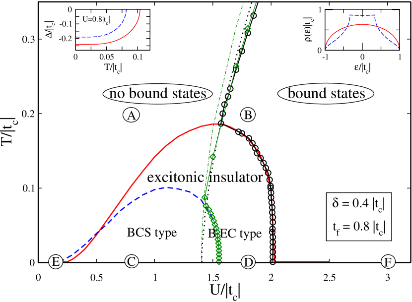
Figure 1: (color online) Phase boundary of the EI phase in the EFKM which typifies either a BEC or BCS condensate. Red solid (blue dashed) lines are obtained using the semielliptic (3D simple cubic) DOS shown in the right inset. The symbols give the critical $U$-values for exciton formation. Note that preformed pairs may exist in the normal phase of the EFKM. Black dotted (green dashed-dotted) lines mark the opening of the gap $E_{g}^{(0)}$ (assuming $\Delta=0$). For further explanation see text. The left inset shows exemplarily the suppression of the order parameter $\Delta$ with increasing temperature on the track from C $\to$ A, i.e. at fixed $U$, where a second-order phase transition is obtained.

Thus, the existence or non-existence of bound states above $T_{c}$ gives strong evidence for a BEC or BCS transition scenario at $T_{c}$, respectively. Moreover, within the EI phase, a crossover from a strong-coupling BEC to a weak-coupling BCS condensate of electron-hole pairs is strongly suggested.

To describe qualitatively this BEC-BCS crossover region, we consider the gap boundary $U_{g}(T)$ (thin dotted and dashed-dotted lines) resulting from $E_{g}^{(0)}=0$ [Eq. (7)], where the gap opens for $U>U_{g}$. Interestingly, at $T_{s}=T_{c}(U_{s})$ we obtain $U_{g}(T_{s})=U_{X}(T_{s})$. That is, at this point the opening of the gap is accompanied with the formation of bound states, whereas for $T>T_{c}$, $U_{g}(T)$ is slightly smaller than $U_{X}(T)$. From this result we may get a crude estimate of the BEC-BCS crossover region by extrapolating $U_{g}(T)$ into the EI phase. Solving Eq. (6) at a fixed $T<T_{c}$, for $U$ in the region $U_{g}<U<U_{X}$ we get negative pole energies $\omega_{X}$ which indicates the instability of the normal phase with bound states against the long-range ordered EI phase. Moreover, for $U\lesssim U_{g}$ no solution can be found which may be indicative for an instability towards a BCS-type EI state. Thus, the BEC-BCS crossover in the EI phase should occur in the neighborhood of the $U_{g}(T)$ line.

In comparison to the phase boundary obtained within the simple effective-mass, Mott-Wannier-type model Bronold and Fehske (2006); Bronold et al. (2007) the EI phase of the EFKM is confined at zero temperature on the weak-coupling side, because of the finite f- and c-bandwidths. While the shape of the EI dome approximates the Tm[Te,Se] phase diagram constructed from the experimental data, the absolute transition temperatures are overestimated, of course, by any mean-field approach. The homogeneous EI phase shrinks as $\delta$ as $t_{f}$ becomes smaller at fixed $\delta$, but it does not disappear. Farkašovský (2008)

Figure 2 gives the partial f- and c-electron DOS at various characteristic points A-F of the phase diagram shown in Fig. 1. The high-temperature phase may be viewed as a metal/semimetal (panel A) or a semiconductor (panel B) in the weak- or intermediate-to-strong interaction regime, respectively. The EI phase shows completely different behavior. As can be seen from panel C, a correlation-induced “hybridization” gap opens, indicating long-range order (non-vanishing f-c-polarization). As the temperature increases the gap weakens and finally closes at $T=T_{c}$. The pronounced c-f-state mixing and strong enhancement of the DOS at the upper/lower valence/conducting band edges is reminiscent of a BCS-like structure evolving from a (semi-) metallic state with a large Fermi surface above $T_{c}$ (see panel A). This may be in favor of a BCS pairing in the weak-coupling region of the EI phase, as discussed above. By contrast the DOS shown in panel D clearly evolves from a gapped high-temperature phase. Finally, in panel E [F] the partial f- and c-electron DOS at $T\simeq 0$ below [above] the EI phase are depicted, where the system behaves as a metal or semimetal [band insulator or semiconductor]. Note that the splitting of c- and f-bands in panel F is not caused by $\delta$ (being the same as in E), but is due to the Hartree shift $\propto U(n_{f}-n_{c})$.

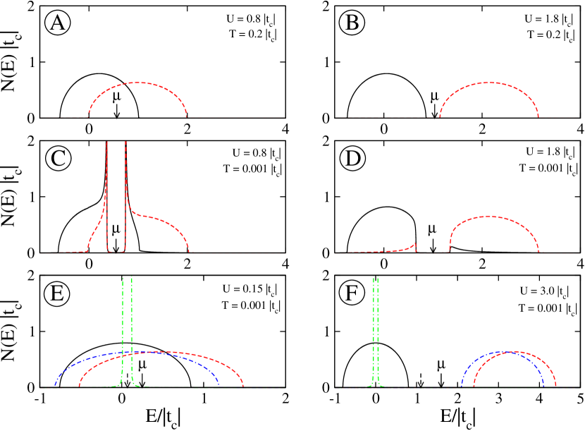
Figure 2: (color online) DOS for f-band ([black] solid curves) and c-band electrons ([red] dashed curves) at the points marked by A to F in the $T$-$U$ plane in Fig. 1. Band structure parameters are $\delta=0.4|t_{c}|$, $t_{f}=0.8|t_{c}|$. For comparison, the results for $\delta=0.1|t_{c}|$ and $t_{f}=0.05|t_{c}|$ ([green] double-dot-dashed and [blue] dot-dashed curves) have been included in panels E and F; here a CDW will become the Hartree-Fock ground state as $U$ increases from E to F. All data are obtained for the semielliptic DOS and total filling $n=n_{f}+n_{c}=1$; the arrows mark the positions of the chemical potential.

To summarize, in this work, we attempted to link experimental hints for excitonic condensation to recent theoretical studies of electronic ferroelectricity in the extended Falicov-Kimball model. We analyzed the finite-temperature phase diagram and argued that a finite f-bandwidth in combination with a short-range interband Coulomb attraction between (heavy) valence-band holes and (light) conduction-band electrons may lead to f-c-band coherence and an excitonic insulator low-temperature phase. Most noteworthy we established the existence of excitonic bound states for the EFKM on the semiconductor side of the semimetal semiconductor transition above $T_{c}$, and suggested a BCS-BEC crossover scenario within the condensed state. As a consequence, we expect pronounced transport anomalies in the transition regime both in the low- and high-temperature phases, which should be studied in the framework of the EFKM in future work.

Acknowledgments. This work was supported by DFG through SFB 652. The authors thank B. Bucher and A. Weiße for helpful discussions.

References

- Knox (1963) R. Knox, in Solid State Physics, edited by F. Seitz and D. Turnbull (Academic Press, New York, 1963), p. Suppl. 5 p. 100; L. V. Keldysh and H. Y. V. Kopaev, Sov. Phys. Sol. State 6, 2219 (1965); D. Jérome, T. M. Rice, and W. Kohn, Phys. Rev. 158, 462 (1967).
- Littlewood et al. (2004) P. B. Littlewood, P. R. Eastham, J. M. J. Keeling, F. M. Marchetti, B. D. Simons, and M. H. Szymanska, J. Phys. Condens. Matter 16 (2004).
- Neuenschwander and Wachter (1990) J. Neuenschwander and P. Wachter, Phys. Rev. B 41, 12693 (1990); B. Bucher, P. Steiner, and P. Wachter, Phys. Rev. Lett. 67, 2717 (1991); P. Wachter, Solid State Commun. 118, 645 (2001); B. Bucher, T. Park, J. D. Thompson, and P. Wachter (2008), URL arXiv:0802.3354[cond-mat.str-el].
- Wachter et al. (2004) P. Wachter, B. Bucher, and J. Malar, Phys. Rev. B 69, 094502 (2004).
- Bronold and Fehske (2006) F. X. Bronold and H. Fehske, Phys. Rev. B 74, 165107 (2006).
- Bronold et al. (2007) F. X. Bronold, G. Röpke, and H. Fehske, J. Phys. Soc. Jpn., Suppl. A 76, 27 (2007); F. X. Bronold and H. Fehske, Superlattices and Microstructures 43, 512 (2008).
- Rice (1963) T. M. Rice, in Solid State Physics, edited by F. Seitz, D. Turnbull, and H. Ehrenreich (Academic Press, New York, 1963), p. Vol. 32 pp. 1.
- Bonitz et al. (2005) M. Bonitz, V. S. Filinov, V. E. Fortov, P. R. Levashov, and H. Fehske, Phys. Rev. Lett. 95, 235006 (2005).
- Cercellier et al. (2007) H. Cercellier et al., Phys. Rev. Lett. 99, 146403 (2007); C. Monney et al., URL arXiv:0809.1930.
- Falicov and Kimball (1969) L. M. Falicov and J. C. Kimball, Phys. Rev. Lett. 22, 997 (1969).
- Ramirez et al. (1970) R. Ramirez, L. M. Falicov, and J. C. Kimball, Phys. Rev. B 2, 3383 (1970).
- Portengen et al. (1996a) T. Portengen, T. Östreich, and L. J. Sham, Phys. Rev. Lett. 76, 3384 (1996a); Phys. Rev. B 54, 17452 (1996b).
- Czycholl (1999) G. Czycholl, Phys. Rev. B 59, 2642 (1999).
- Farkašovský (2008) P. Farkašovský, Phys. Rev. B 59, 9707 (1999).
- Batista (2002) C. D. Batista, Phys. Rev. Lett. 89, 166403 (2002).
- Batista et al. (2004) C. D. Batista, J. E. Gubernatis, J. Bonča, and H. Q. Lin, Phys. Rev. Lett. 92, 187601 (2004).
- Farkašovský (2008) P. Farkašovský, Phys. Rev. B 77, 155130 (2008).
- Schneider and Czycholl (2008) C. Schneider and G. Czycholl, Eur. Phys. J. B 64, 43 (2008).
- Brydon (2008) P. M. R. Brydon, Phys. Rev. B 77, 045109 (2008).
- Gasser et al. (2001) W. Gasser, E. Heiner, and K. Elk, Greensche Funktionen in Festkörper- und Vielteilchenphysik (WILEY-VCH Verlag, Berlin, 2001).
- Nozieres (1985) P Nozierès and S. Schmitt-Rink, J. Low Temp. Phys. 59, 195 (1985).