Noise in an SSET-resonator driven by an external field

Abstract

We investigate the noise properties of a superconducting single electron transistor (SSET) coupled to an harmonically driven resonator. Using a Langevin equation approach, we calculate the frequency spectrum of the SSET charge and calculate its effect on the resonator field. We find that the heights of the peaks in the frequency spectra depend sensitively on the amplitude of the resonator oscillation and hence suggest that the heights of these peaks could act as a sensitive signal for detecting the small changes in the amplitude of the drive. The previously known results for the effective amplitude-dependent damping and temperature provided by the SSET for the case of a low frequency resonator are generalized for all resonator frequencies.

Over the past few years experiments on superconducting circuits have produced some rather impressive results. Superconducting elements have been used to produce two-level systems of various kinds which can be considered as artificial atoms Nakamura ; Martinis ; Cottet ; Mooij , and superconducting stripline resonators can act analogously to optical cavities for microwave fields SCR . This field of study has been referred to as circuit QED in analogy with cavity QED. One advantage of superconducting circuits is that rather than simply investigating the behavior of the system through the field emitted or reflected by the cavity, other elements can provide additional information. Mesoscopic conductors coupled to the resonator can provide additional information and at the same time the back action may lead to some interesting and subtle dynamics. Such back-action dynamics have also received considerable attention in the context of a mesoscopic conductor used to investigate the behavior of a mechanical resonator Blencowe ; MM ; CG ; Swede ; mmh ; ABZ ; SET-expt ; ra .

One system that is of particular interest is that of a superconducting single electron transistor (SSET) coupled to a resonator, either mechanical bia ; SSET1 ; bc ; SSET-expt2 ; SSET-expt ; ria ; riha or composed of a superconducting stripline Tsai07 . The coherent transport through this device at the Josephson quasiparticle resonance Choi ; CSSET (JQP) allows a very low-noise current, and at the same time the sensitivity of the SSET to charge means that the resonator-SSET coupling is significant. The SSET biased at the JQP resonance can be considered analogous to a three-level atom, and the coupled system therefore shows behavior related to that of a micromaser micromaser ; micromaser_review .

The low noise and relatively strong coupling in this device allows the observation of the non-trivial coupled dynamics that arises from the interaction between the resonator and SSET. When the SSET is biased so as to absorb energy from the resonator, the SSET acts as an additional source of damping, and the resonator can be cooled below its physical temperature. This modification of the steady state of the resonator due to a back-action induced effective damping and temperature has been observed for an SSET coupled to both mechanical and superconducting resonators SSET-expt2 ; Tsai07 . When the SSET is biased to the other side of the JQP resonance, energy is transferred from the SSET to the resonator, leading to an effective negative damping. For a superconducting stripline resonator, the quality factor can be high enough that the negative damping dominates and the resonator is driven into an oscillating state even in the absence of an external drive ria ; bc ; Hauss . This has recently been observed for a superconducting stripline resonator coupled to an SSET, and the field transmitted through the resonator measured Tsai07 . When the resonator is in this oscillating state, the SSET has a periodic but not harmonic response, with the details of its dynamics depending rather sensitively on the amplitude of the resonator oscillation. In order to probe this behavior, we must go beyond the time-averaged mean field behaviour riha and investigate the correlations present in the system.

With a stripline resonator, as opposed to a mechanical one, there are two independent probes of the system - the field in the superconducting stripline, and the current that passes through the SSET. This then allows the investigation of the system by two different experimental methods. The noise properties of the SSET-cavity system are transferred to both the current and reflected field, so we can consider these to be probing the noise present in our system. The effect of the thermal noise in both the SSET and the cavity can be made very small, so the noise detected largely arises from the finite level structure of the SSET, and is in that sense is a purely quantum noise.

In this paper, we consider an SSET that is coupled to a resonator that is driven into an oscillating state. We calculate the charge noise on the SSET and the effect this has on the cavity field. We also consider the case when the resonator’s motion depends on the effective damping and noise arising from the SSET, using a linear response approach Clerk . We go on to show how the response of the system at the sidebands could be used to detect small changes in the driving amplitude. Although we focus our analysis on the case of a superconducting stripline, which has a higher oscillation frequency, our main results are also valid for the lower frequency mechanical resonators. In our calculation, we take advantage of the fact that the resonator oscillations change on a timescale that is slow compared to the SSET timescales, which is valid as long as the resonator damping and coupling to the SSET are weak. This means that the SSET response is essentially the response to a purely harmonic drive. This approach has previously been used for both mechanical and optomechanical systems riha ; MHG . However, by including a fluctuating Langevin term, we can go beyond the previous mean field results to calculate the noise. The effect of this response on the resonator can then be calculated.

In Sec. I we introduce our model of the system and Langevin equations for the resonator field and the SSET variables. In Sec. II we introduce the main approximations made and solve the Langevin equations for the SSET under the influence of the periodic driving provided by the resonator. Section III describes the frequency spectrum of the charge on the SSET and gives approximate expressions valid when the resonator frequency is large. In Sec. IV we show how the charge dynamics affect the field in the cavity. We derive expressions for the effective SSET damping and temperature of the resonator, going beyond previously published results to derive expressions valid for all resonator frequencies. Section V describes how the response of the system at multiples of the resonator frequency could be used to detect small changes in the driving amplitude and Section VI describes how the field in the cavity could be measured through a transmission line coupled to the cavity. In Sec. VII we present our conclusions and in appendix A we present more details of the derivation of the Langevin equations for the SSET.

I Master Equation and Langevin Equations

The master equation for a superconducting single electron transistor biased at the Josephson quasiparticle resonance and capacitively coupled to a resonator bia ; ria ,

$$\dot{\rho}={\mathcal{L}}\rho=-\frac{i}{\hbar}[H_{\rm co},\rho]+\mathcal{L}_{leads}\rho+\mathcal{L}_{damping}\rho.$$ (1)

consists of a coherent part, described by the Hamiltonian, $H_{\rm co}$, together with two dissipative terms $\mathcal{L}_{leads}$ and $\mathcal{L}_{damping}$ which describe quasiparticle decay from the island and the surroundings of the resonator respectively. The effective Hamiltonian is given by,

$$H_{\rm co} = -\hbar\Delta\sigma_{22}-\hbar\epsilon_{J}\left(\sigma_{02}+\sigma_{20}\right)$$ (2)

$$+\hbar\omega_{0}a^{{\dagger}}a+\hbar A_{D}(ae^{i\omega_{D}t}+a^{\dagger}e^{-i\omega_{D}t})$$

$$-\hbar\omega_{0}\frac{x_{s}}{2x_{q}}(a+a^{\dagger})\left(\sigma_{11}+2\sigma_{22}\right),$$

where the operators $\sigma_{ij}=|i\rangle\langle j|$ represent operators on the SSET island charge states $|i\rangle$, $\Delta$ is the energy difference between states $|2\rangle$ and $|0\rangle$ and $\epsilon_{J}$ is the Josephson energy of the superconductor. The frequency of the resonator is $\omega_{0}$ and $A_{D},\omega_{D}$ give the strength and frequency of the external driving respectively. The resonator-SSET coupling is described by the parameter $x_{s}$ which measures the shift in the equilibrium field of the resonator brought about by adding a single electronic charge to the SSET island bia , and $x_{q}=(\hbar/2\epsilon_{0}\omega_{0})^{\frac{1}{2}}$. The tunneling of quasiparticles from the island is described by

$$\mathcal{L}_{leads}\rho = -\frac{\Gamma}{2}\left[\left\{\sigma_{22}+\sigma_{11},\rho\right\}_{+}\right.$$

$$\left.-2\left(\sigma_{12}+\sigma_{01}\right)\rho\left(\sigma_{21}+\sigma_{10}\right)\right],$$

where we have neglected the position dependence of the tunnel rates as being of lesser importance than the coherent coupling ria ; riha . This simplification means that the dissipation takes a Lindblad form, and also means that the master equation is essentially equivalent to that of a resonator coupled to a double quantum dot. The dissipation and fluctuations arising from the resonator’s surroundings are described by the usual quantum optical expression WM ,

$$\mathcal{L}_{damping}\rho = -\frac{\gamma_{ex}}{2}(\overline{n}+1)\left(a^{\dagger}a\rho+\rho a^{\dagger}a-2a\rho a^{\dagger}\right)$$

$$-\frac{\gamma_{ex}}{2}\overline{n}\left(aa^{\dagger}\rho+\rho aa^{\dagger}-2a^{\dagger}\rho a\right)$$

where this form for the dissipation is valid as long as the dynamics of the system are slow compared to the correlation time of the bath.

An alternative description of the system is given by a set of Langevin equations describing the coupled system. This gives an equivalent description of the first and second moments of the system, which is what is required for a noise calculation. We shall see later that this Langevin form is convenient for dealing with the external drive, as a transformation can be made which allows us to solve the equation analytically.

The Langevin equations are equal to the semiclassical equations plus a fluctuating noise term. For the resonator operator $a$ we have,

$$\dot{a} = -i\omega_{0}a-\frac{\gamma_{ex}}{2}a-iA_{D}e^{-i\omega_{D}t}+\eta_{a}$$ (5)

$$+i\omega_{0}\frac{x_{s}}{2x_{q}}(\sigma_{11}+2\sigma_{22})$$

where $\eta_{a}$ represents the standard white noise term on the resonator defined by ${\left\langle\eta_{a}(t)\right\rangle}=0$ , ${\left\langle\eta_{a}^{\dagger}(t)\eta_{a}(t^{\prime})\right\rangle}=\delta(t-t^{\prime})\gamma_{ex}\bar{n}$ and ${\left\langle\eta_{a}(t)\eta_{a}^{\dagger}(t^{\prime})\right\rangle}=\delta(t-t^{\prime})\gamma_{ex}(\bar{n}+1)$. This couples to the equations for the SSET charge operators $\sigma_{ij}={|i\rangle}{\langle j|}$ riha . The Langevin equations for the projection operators are given by,

$$\dot{\sigma}_{00}(t) = i\epsilon_{J}(\sigma_{02}(t)-\sigma_{20}(t))+\Gamma\sigma_{11}(t)+\eta_{00}(t).$$ (6)

$$\dot{\sigma}_{11}(t) = \Gamma\sigma_{22}(t)-\Gamma\sigma_{11}(t)+\eta_{11}(t)$$ (7)

$$\dot{\sigma}_{22}(t) = -i\epsilon_{J}(\sigma_{02}(t)-\sigma_{20}(t))-\Gamma\sigma_{22}(t)+\eta_{22}(t)$$ (8)

which also couple to the equation of motion for the off-diagonal terms describing the coherence between levels ${|0\rangle}$ and ${|2\rangle}$,

$$\dot{\sigma}_{02}(t) = -i\epsilon_{J}(\sigma_{22}(t)-\sigma_{00}(t))\!-\!\frac{\Gamma}{2}\sigma_{02}(t)$$

$$+i(\Delta\!+\!\frac{\omega_{0}x_{s}}{x_{q}}(a(t)\!+a^{\dagger}(t)))\sigma_{02}(t)+\eta_{02}(t).$$

We need to find the properties of the correlators for the SSET noise operators $\eta_{ij}$. The Langevin equations, including the properties of the noise operators, can be easily derived from the master equation by requiring that the two forms give the same equations of motion for the second moments of the operators, determining the correlation properties of $\eta_{ij}$ (see appendix A). For example, for the operator representing the noise on $\sigma_{02}$ we have,

$${\left\langle\eta_{02}(t)\eta_{20}(t^{\prime})\right\rangle} = \Gamma({\left\langle\sigma_{00}(t)\right\rangle}+{\left\langle\sigma_{11}(t)\right\rangle})\delta(t-t^{\prime}).$$ (10)

There are a few points to note about the noise operators for the SSET. Firstly, in the limit $k_{B}T\ll\hbar\epsilon_{J}$, the SSET experiences no direct thermal noise. The “noise” terms $\eta_{02}(t)$ therefore arise solely from the finite level structure of the SSET and the resulting commutation relations, and in that sense can be considered to be purely quantum noise. Secondly, we are giving an approximate treatment of this quantum noise by requiring that the first and second order moments calculated by the quantum Langevin equations are equivalent to the first and second order moments as determined by the master equation. In general these would not suffice to determine all the moments in the system. Finally, we note is that we are describing a system under periodic driving which will therefore tend to a periodic behavior in the long time limit, rather than a fixed point. In a finite level system, the correlators involve the average values of the operators such as ${\left\langle\sigma_{11}(t)\right\rangle}$ which depend on $t$ in a driven system. This means that we have time-dependent noise correlators for the SSET noise operators.

The equations for the operators $\sigma_{12}$,$\sigma_{10}$ decouple from the others, so Eqs. (6-I), along with their correlators, completely determine the dynamics of the SSET-resonator system, up to second order.

II Solving the $\sigma_{02}$ Langevin Equation

In this section we solve the Langevin equation (Eq. (I)) for the off-diagonal charge operator $\sigma_{02}$. In order to progress we make two assumptions: first that the Josephson energy is rather small, and second that the amplitude of the resonator changes slowly compared to the incoherent dynamics of $\sigma_{02}$, i.e. that the total damping due to both the resonator environment and the SSET $\gamma_{T}=\gamma_{ex}+\gamma_{SS}$ is much smaller than the quasiparticle decay rate $\Gamma$.

In the limit that the Josephson energy is much weaker than the quasiparticle decay, $\epsilon_{J}\ll\Gamma$, the occupation of the charge states $\sigma_{11},\sigma_{22}\ll 1$, and the equation of motion for $\sigma_{02}$ decouples from the other charge equations. We are assuming the resonator amplitude can be treated as constant on timescales relevant to the SSET dynamics, an approximation which has proved useful in related mechanical and optomechanical systems riha ; MHG . Our derivation closely follows these methods, but also incorporates the fluctuations described by the $\eta$ terms. We replace the term describing the field in Eq. (I) with a cosine oscillation at the driving frequency with magnitude $A$ i.e. $(a(t)+a^{\dagger}(t))\approx A\cos(\omega_{D}t)$. For the case of weak back-action damping, the amplitude is simply given by $A=A_{D}/((\omega_{0}-\omega_{D})^{2}+\gamma_{ex}^{2})^{1/2}$. When the back action damping is significant, the amplitude must be determined self-consistently - an oscillation of amplitude $A$ will be stable if the resulting total damping is zero.

This then means that the field simply appears as an harmonic drive acting on the SSET, and Eq. (I) becomes,

$$\dot{\sigma}_{02}(t)\!\!\! = \!i\epsilon_{J}\!-\!\left(\frac{\Gamma}{2}\!-\!i\Delta\!-\!i\frac{\omega_{0}x_{s}}{x_{q}}A\cos\omega_{D}t\right)\sigma_{02}(t)\!+\eta_{02}(t),$$

where the first term on the right hand side multiplies an implicit identity operator.

If we make a transformation to eliminate the driving term, $\tilde{\sigma}_{02}=\sigma_{02}e^{-iz\sin\omega_{D}t}$, we can then find the Fourier transform of the transformed operator $\tilde{\sigma}_{02}$ in terms of Bessel functions of the first kind, $J_{n}(z)$, where $z=(\omega_{0}x_{s}A)/(\omega_{D}x_{q})$,

$$\tilde{\sigma}_{02}(\omega_{F}) = \frac{i\epsilon_{J}\sum\limits_{n}\delta(\omega_{F}-\omega_{D}n)J_{n}\left(-z\right)}{\Gamma/2+i(\omega_{F}-\Delta)}$$ (12)

$$+\frac{\frac{1}{2\pi}\int\limits_{-\infty}^{\infty}e^{-i\omega_{F}t}e^{-iz\sin\omega_{D}t}\eta_{02}(t){\textrm{d}}t}{\Gamma/2+i(\omega_{F}-\Delta)}$$

and we see that $\tilde{\sigma}_{02}$ consists of a systematic response to the drive at multiples of the driving frequency $\omega_{D}$, plus a noise term.

Equation (12) gives the Fourier component in the transformed picture, so we convert back to the untransformed picture to obtain,

$${\sigma}_{02}(\omega_{F}) = \sum\limits_{n,n^{\prime}}{\frac{i\epsilon_{J}\delta(\omega_{F}-\omega_{D}n^{\prime})J_{n^{\prime}-n}\left({\scriptstyle-}z\right)J_{n}\left(z\right)}{\Gamma/2+i(\omega_{D}(n^{\prime}-n)-\Delta)}}$$

$$+ \sum\limits_{n}\frac{\int\limits_{-\infty}^{\infty}e^{-i(\omega_{F}t-\omega_{D}nt+z\sin\omega_{D}t)}\eta_{02}(t)J_{n}\left(z\right){\textrm{d}}t}{2\pi(\Gamma/2+i(\omega_{F}-\omega_{D}n-\Delta))},$$

which gives an expression for the Fourier transform of $\sigma_{02}(t)$ consisting of a mean field and noise-induced term. From this expression we can go on to calculate the spectrum of the charge on the SSET and hence of the cavity field.

III Noise on the SSET

The frequency spectrum of two fluctuating terms $f(t),g(t)$ is defined by,

$$S_{fg}(\omega,t) = \int\limits_{-\infty}^{\infty}{\textrm{d}}\tau e^{i\omega\tau}{\left\langle f(t+\tau)g(t)\right\rangle}$$ (14)

$$= 2\pi\int\limits_{-\infty}^{\infty}{\textrm{d}}\omega_{F}e^{i(\omega_{F}+\omega)t}{\left\langle f(\omega)g(\omega_{F})\right\rangle}$$

where in the second line we have written the spectrum in terms of the Fourier transforms of the individual functions. Note that as defined, the spectrum includes correlations due to the systematic motion of the terms as well as due to the fluctuations. If the functions $f,g$ are periodic then the above expression retains a periodic time dependence. We therefore define a spectrum averaged over a single driving period, $S_{fg}(\omega)=\frac{\omega_{D}}{2\pi}\int\limits_{-\pi/\omega_{D}}^{\pi/\omega_{D}}{\textrm{d}}tS_{fg}(\omega,t)$, which is what we would expect to observe in experiment. Inserting Eq. (LABEL:eq:FTp02) into this expression and noting that in the small-$\epsilon_{J}$ limit we can approximate the time dependent correlator given in Eq. (10) as ${\left\langle\eta_{02}(t)\eta_{20}(t^{\prime})\right\rangle}\approx\Gamma\delta(t-t^{\prime})$, gives,

$$S_{\sigma_{02}\sigma_{20}}(\omega)\! = \!\sum\limits_{n}2\pi\delta(\omega\!-\!\omega_{D}n)\left|\sum\limits_{n^{\prime}}\frac{\epsilon_{J}J_{n^{\prime}}\left(\text{-}z\right)J_{n\text{-}n^{\prime}}\left(z\right)}{\frac{\Gamma}{2}+i(\omega_{D}n^{\prime}-\Delta)}\right|^{2}$$ (15)

$$+\sum\limits_{n}\frac{\Gamma J_{n}\left(z\right)^{2}}{(\omega-\omega_{D}n-\Delta)^{2}+\Gamma^{2}/4}.$$

The first term corresponds to the correlations arising from the systematic response of the resonator to the driving force. For a purely monochromatic drive, the peaks are $\delta-$functions, but in reality the $\delta-$functions would be replaced by peaks with total power unity and a width determined by the linewidth of the driving. The second term describes the additional noise due to the finite level structure.

We have calculated the noise on the off-diagonal element of the SSET density matrix, $\sigma_{02}$. However, this does not enter directly into the current or cavity noise. Instead, we have to calculate the frequency spectrum of the total charge on the SSET, $\sigma_{cc}=\sigma_{11}+2\sigma_{22}$.

III.1 Systematic Charge Oscillations

Fourier transforming Eqs. (6-8) gives an expression for the charge in terms of $\sigma_{02}(\omega_{F})$. Inserting Eq. (15) into this gives an expression for the charge consisting of a systematic part, and a fluctuating part containing the noise operators $\eta_{02},\eta_{11}$ and $\eta_{22}$. We now go on to calculate the fluctuation spectrum of the charge due to the systematic and noisy terms.

The systematic component of the charge, $\sigma_{02}^{S}(\omega_{F})$ is given by,

$$\sigma^{S}_{cc}(\omega_{F}) = \frac{(3\Gamma+2i\omega_{F})\epsilon_{J}^{2}}{(\Gamma+i\omega_{F})^{2}}\sum\limits_{n,n^{\prime}}J_{n^{\prime}}\left(z\right)\delta(\omega_{F}-\omega_{D}n)$$

$$\times\left(\frac{J_{n^{\prime}+n}\left(z\right)}{\frac{\Gamma}{2}-i(\omega_{D}n^{\prime}\!+\!\Delta)}+\frac{J_{n^{\prime}\text{-}n}\left(z\right)}{\frac{\Gamma}{2}+i(\omega_{D}n^{\prime}\!+\!\Delta)}\right),$$

and we see that the mean field response of the charge is a series of $\delta-$peaks at multiples of $\omega_{D}$.

The systematic motion of the charge will show up in the time correlation function and hence the fluctuation spectrum. We insert Eq. (LABEL:eq:p11p22FTS) into Eq. (14) to obtain the part of the charge spectrum due to systematic evolution,

$$S^{S}_{cc}(\omega) = \sum\limits_{n}2\pi\delta(\omega+n\omega_{D})\epsilon_{J}^{4}\frac{9\Gamma^{2}+4\omega_{D}^{2}n^{2}}{(\Gamma^{2}+\omega_{D}^{2}n^{2})^{2}}$$

$$\times \!\left|\sum_{n^{\prime}}\left(\frac{J_{n^{\prime}}\!\left(z\right)J_{n+n^{\prime}}\left(z\right)}{\frac{\Gamma}{2}-i(\omega_{D}n^{\prime}\!+\!\Delta)}+\frac{J_{n^{\prime}}\!\left(z\right)J_{n^{\prime}\text{-}n}\left(z\right)}{\frac{\Gamma}{2}+i(\omega_{D}n^{\prime}\!+\!\Delta)}\right)\right|^{2}$$

For $\Gamma,\Delta\ll\omega_{D}$, this expression is dominated by the $n^{\prime}=0$ term in the sum, and the systematic noise reduces to,

$$S^{S}_{cc}(\omega) \approx \sum\limits_{n}2\pi\delta(\omega+n\omega_{D})\epsilon_{J}^{4}\frac{4}{(\omega_{D}n)^{2}}J_{0}\left(z\right)^{2}$$ (18)

$$\times\left|\left(\frac{J_{n}\left(z\right)}{\frac{\Gamma}{2}-i\Delta}+\frac{J_{-n}\left(z\right)}{\frac{\Gamma}{2}+i\Delta}\right)\right|^{2}$$

The symmetry properties of the Bessel functions then mean that the bessel functions will either add or cancel depending on whether $n$ is odd or even, so separating out the two cases we find,

$$S^{S}_{cc}(\omega) \approx \frac{4\epsilon_{J}^{4}J_{0}\left(z\right)^{2}}{(\Delta^{2}+\frac{\Gamma^{2}}{4})^{2}}\sum\limits_{n}\frac{2\pi\delta(\omega+n\omega_{D})}{(\omega_{D}n)^{2}}J_{n}\left(z\right)^{2}$$

$$\times\left(\Gamma^{2}\frac{(1+(-1)^{n})}{2}+4\Delta^{2}\frac{(1-(-1)^{n})}{2}\right)$$

III.2 Charge Spectrum Due to Fluctuations

As well as the systematic response to the driving force, the charge spectrum also contains a part due to fluctuations. The Fourier transform of the charge $\sigma_{cc}=\sigma_{11}+2\sigma_{22}$ contains the fluctuating terms corresponding to both the diagonal and off-diagonal operators, $\eta_{11},\eta_{22},\eta_{02}$. Inserting these into Eq. (14), we write the fluctuation-induced part of the charge spectrum as,

$$S^{\eta}_{cc} = S^{diag}_{cc}+S^{\eta_{02},\eta_{20}}_{cc}+S^{cross}_{cc}$$ (20)

where $S^{diag}_{cc}$ corresponds to the part arising from fluctuations on the diagonal operators $\eta_{11},\eta_{22}$, the term $S^{02}_{cc}$ arises from $\eta_{02}$, and $S^{cross}_{cc}$ from the correlations between these. Note that while ${\left\langle\eta_{02}(t)\eta_{20}(t^{\prime})\right\rangle}$ can be approximated to a constant in the small-$\epsilon_{J}$ limit, other correlators give, for example, ${\left\langle\eta_{22}(t)\eta_{22}(t^{\prime})\right\rangle}=\Gamma{\left\langle\sigma_{22}(t)\right\rangle}\delta(t-t^{\prime})$, i.e. we have a time dependent function multiplied by a delta function. As ${\left\langle\sigma_{22}(t)\right\rangle}$ is simply the systematic part of $\sigma_{22}$, we can insert the Fourier transform of this into our calculation. After some algebra, we find,

$$S_{cc}^{diag}(\omega) = \frac{5\Gamma^{2}+2\omega^{2}}{(\Gamma^{2}+\omega^{2})^{2}}\sum\limits_{n}\frac{J_{n}\left(z\right)^{2}\Gamma\epsilon_{J}^{2}}{\frac{\Gamma^{2}}{4}+(\omega_{D}n+\Delta)^{2}}$$ (21)

$$S_{cc}^{\eta_{02},\eta_{20}}(\omega) = \frac{9\Gamma^{2}+4\omega^{2}}{(\Gamma^{2}+\omega^{2})^{2}}\sum\limits_{n}\frac{J_{n}\left(z\right)^{2}\Gamma\epsilon_{J}^{2}}{\frac{\Gamma^{2}}{4}+(\omega-\omega_{D}n-\Delta)^{2}}$$

. (22)

The expression for the cross terms is rather unwieldy, but can be written as,

$$S_{c,c}^{cr}(\omega) = \Re\Bigg{\{}\frac{12\Gamma^{2}+4\omega^{2}+2i\omega\Gamma}{(\Gamma^{2}+\omega^{2})^{2}}$$

$$\times \sum\limits_{n}\frac{J_{n}\left(z\right)^{2}\Gamma\epsilon_{J}^{2}}{(\frac{\Gamma}{2}-i(\omega_{D}n\!-\!\Delta))(\frac{\Gamma}{2}+i(\omega-\!\omega_{D}n-\!\Delta))}\Bigg{\}}$$

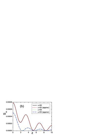
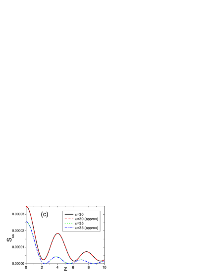
In Fig. 1 we plot the charge noise as a function of $\omega$, and see it consists of a series of peaks (of width $\sim\Gamma$) at integer multiples of the driving frequency on top of a background peak centered on $\omega=0$.

Figure 1: (color online). Charge noise as a function of $\omega$ for different driving frequencies $\omega_{D}=(a)0.5,(b)2,(c)10$ relative to the quasiparticle decay $\Gamma$. The different curves show different driving amplitudes $z=2,3,4$. The inset (d) in the $\omega_{D}=10$ plot shows that the large central peak is highly suppressed at $J_{0}(z)=0$, here at $z=2.4048$. The other parameters are $\epsilon_{J}=1/16,\Gamma=1,\Delta=-0.5,$

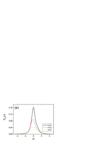
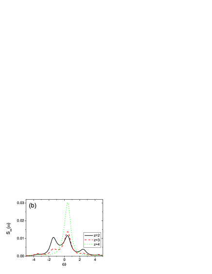
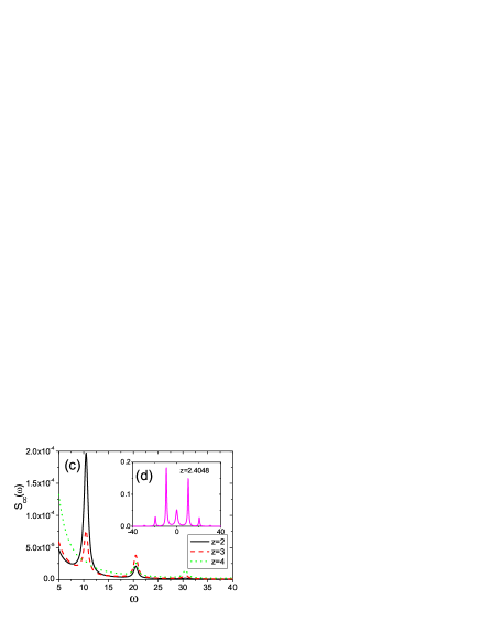
It is these sideband peaks that give information about the driving frequency and amplitude, and so we would like to find some simple expressions that tell us if these peaks can be observed. The peaks are more pronounced in the limit that the resonator frequency is larger than the quasiparticle decay rate, and this is what we would expect to be the case experimentally for superconducting stripline resonators.

The spectrum simplifies considerably in the large $\omega_{D}$ limit. The diagonal term, Eq. (21), consists of a peak at $\omega=0$, multiplied by a sum that is independent of $\omega$. We can approximate the sum by the $n=0$ term in the $\Gamma,\Delta\ll\omega_{D}$ limit to obtain,

The other terms describe a similar peak at $\omega=D$, multiplied by a series of peaks. We wish to find an expression for the heights of these peaks. In the $\Gamma,\Delta\ll\omega_{D}$ limit, we find that the heights of the noise terms at integer values of the driving frequency are,

$$S^{\eta_{02},\eta_{20}}_{cc}(\omega_{D}n) \approx \frac{4J_{n}(z)^{2}}{(\omega_{D}n)^{2}}\frac{\Gamma\epsilon_{J}^{2}}{\frac{\Gamma^{2}}{4}+\Delta^{2}}$$

$$S^{cr}_{cc}(\omega_{D}n) \approx -\frac{4J_{n}(z)^{2}\Delta}{(\omega_{D}n)^{3}}\frac{\Gamma\epsilon_{J}^{2}}{\frac{\Gamma^{2}}{4}+\Delta^{2}}$$ (24)

and we note that the cross terms are negligible in this limit and can be neglected. Thus we can write the height of the charge peaks as

$$S^{\eta}_{cc}(\omega_{D}n) \approx \frac{(4J_{n}(z)^{2}+2J_{0}(z)^{2})}{2\pi(\omega_{D}n)^{2}}\frac{\Gamma\epsilon_{J}^{2}}{\frac{\Gamma^{2}}{4}+\Delta^{2}}.$$ (25)

The visibility of the peaks depends on the contrast between the noise at the peaks and the noise between the peaks Doiron2QPC .

Between the peaks, two terms in the sum are relevant which gives, to leading order,

$$S^{\eta}_{cc}(\omega_{D}(n+\frac{1}{2})) \approx \frac{2J_{0}(z)^{2}}{\omega_{D}^{2}(n+\frac{1}{2})^{2}}\frac{\Gamma\epsilon_{J}^{2}}{\frac{\Gamma^{2}}{4}+\Delta^{2}}$$ (26)

The ratio reaches a minimum when $J_{n}(z)=0$, at which point we see the ratio is $(n+\frac{1}{2})^{2}/n^{2}$. The ratio becomes large when $J_{0}(z)=0$, and is of order $\omega_{D}^{2}n^{2}/(\frac{\Gamma^{2}}{4}+\Delta^{2})$. Examples of the on- and off-peak heights as a function of the driving are shown in Fig. (2), along with the approximations to these given in Eqs. (25-26).

$$S^{diags}_{cc}(\omega) \approx \frac{5\Gamma^{2}+2\omega^{2}}{(\Gamma^{2}+\omega^{2})^{2}}\frac{J_{0}(z)^{2}\Gamma\epsilon_{J}^{2}}{\frac{\Gamma^{2}}{4}+\Delta^{2}}$$

Figure 2: (color online). Comparison of the heights of the peaks at $\omega=\omega_{0}n$ and the troughs at $\omega=\omega_{0}(n+1/2)$, for $n=(a)1,(b)2,(c)3$ respectively. Both the full calculated value and the $\Gamma,\Delta\ll\omega_{0}$ approximation are plotted. Parameters: $\omega_{0}=10,\Gamma=1,\Delta=0,\epsilon_{J}=1/16,$

IV Cavity Field

We now consider the effect of the SSET on the cavity. We recall the Langevin equation for the cavity field,

$$\dot{a} = -i\omega_{0}a-\frac{\gamma_{ex}}{2}a-iA_{D}e^{-i\omega_{D}t}+\eta_{a}$$ (28)

$$+i\omega_{0}\frac{x_{s}}{2x_{q}}(\sigma_{11}+2\sigma_{22})$$

where $A_{D}$ represents the amplitude of the classical driving field.

If we neglect the back-action as weak, then the steady state amplitude $A=|a|$ of the resonator is simply given by,

$$A = \frac{A_{D}}{\sqrt{(\omega_{0}-\omega_{D})^{2}+\frac{\gamma_{ex}^{2}}{4}}}.$$ (29)

We can now use this amplitude to calculate the behavior of the SSET. If the back-action of the SSET on the resonator is weak, then the oscillations of the resonator at the driving frequency will be relatively unaffected and hence the drive the SSET field feels will be unchanged. However, the SSET does not simply respond at the driving frequency, but has a systematic response at multiples of $\omega_{D}$, and will also act as an additional source of noise.

Assuming that the response of the SSET at the driving frequency is unaffected by the back-action, the Fourier transform of $a$ is given by,

$$a(\omega_{F}) = \frac{-iA_{D}\delta(\omega_{F}+\omega_{D})+i\omega_{0}\frac{x_{s}}{2x_{q}}\sigma_{cc}^{S}(\omega_{F})}{i(\omega_{F}+\omega_{0})+\frac{\gamma_{ex}}{2}}$$

$$+\frac{\frac{1}{2\pi}\int e^{-i(\omega_{D}+\omega_{F})t}\eta_{a}(t){\textrm{d}}t+i\omega_{0}\frac{x_{s}}{2x_{q}}\sigma_{cc}^{\eta}(\omega_{F})}{i(\omega_{F}+\omega_{0})+\frac{\gamma_{ex}}{2}}$$

where the first line describes the systematic motion of the cavity and the second gives the noise. We now see that our assumption that the change in the oscillation amplitude (i.e. the change of $a(\omega_{D})$) is negligible will be justified whenever $A_{D}\gg\omega_{0}\frac{x_{s}}{x_{q}}\sigma_{cc}^{S}(-\omega_{D})$. At other frequencies the SSET may have a significant effect on the resonator. The systematic response of the resonator at frequency $\omega$ is just the charge response at that frequency multiplied by a prefactor of magnitude $\omega_{0}/((\omega-\omega_{0})^{2}+\gamma_{ex}^{2})^{2}$.

We can now write the cavity noise as a function of the charge noise,

$$S_{a^{\dagger},a}(\omega)=\frac{\bar{n}\gamma_{ex}+\frac{\omega_{0}^{2}x_{s}^{2}}{4xq^{2}}(S^{S}_{c,c}(\omega)+S^{\eta}_{c,c}(\omega))}{(\omega-\omega_{0})^{2}+\frac{\gamma_{ex}^{2}}{4}}$$ (31)

with the systematic and noise-induced parts of the charge spectrum calculated driving amplitude $A$. We see that the charge noise spectrum appears directly in the expression for the cavity noise, and so the sidebands discussed in Sec. III should also be present. Although the size of the peaks is suppressed, we find that (for $\bar{n}=0$), the ratio of the on- and off-peak noise is unchanged.

IV.1 Back-action damping and temperature

In the preceding section, we assumed that the back-action was weak enough that the SSET damping could be neglected. However, it is well known that the effect of the back action on the dynamics of the resonator can be significant. In particular, as well as providing an additional source of noise for the resonator, the SSET can also act to provide an additional source of damping bia ; ria ; riha ; bc ; SSET1 . In these situations, this effective damping will have a significant effect on the noise properties of the resonator even when the resonator is strongly driven. Furthermore, the SSET can cause the total resonator damping of the resonator to become negative, and hence the resonator can be driven into a self-oscillating laser-like state even in the absence of external driving bc ; SSET1 ; ria ; riha . In this section we review how the systematic response of the SSET can act as an amplitude-dependent damping of the resonator, and present some simple analytic approximations before describing how this influences the cavity noise spectrum. We show that the calculation of charge noise presented in Sec. III can be used to generalize the previously known expressions for the effective damping and temperature of a slow ($\omega_{0}\ll\Gamma$) resonator to arbitrary frequency using a linear-response-like approach Clerk .

The calculation of the damping proceeds as follows; the resonator amplitude changes only slowly, so we can average the effect of the systematic SSET motion over a single resonator period. Following the calculation given in riha we obtain an expression for the amplitude-dependent frequency shift and damping introduced by the SSET,

$$(\gamma_{SS}(z)+i\delta\omega_{0}(z))a=$$

$$i\frac{x_{s}\omega_{0}}{2x_{q}}\frac{(3\Gamma+2i\omega_{D})\epsilon_{J}^{2}}{(\Gamma+i\omega_{D})^{2}}\sum\limits_{n}J_{-n}\left(z\right)J_{1-n}\left(z\right)$$

$$\times\left(\frac{1}{\frac{\Gamma}{2}+i(\omega_{D}n-\Delta)}-\frac{1}{\frac{\Gamma}{2}+i(\omega_{D}n+\Delta)}\right)$$

In Fig. 3(a) we plot the damping as a function of amplitude. The resonator $A$ amplitude is then found by solving the self consistent equation for $a$ in the rotating frame,

$$0 = -i(\omega_{0}-\omega_{D})a-\gamma_{ex}a+iA_{D}$$ (33)

$$-(\gamma_{SS}(z)+i\delta\omega_{0}(z))a.$$

Figure 3: (color online). Plot of the SSET damping. Plot (a) shows non-linear damping, with $-\gamma_{SS}A$ plotted against $A$. Plotted are the full expression for the damping, $\gamma_{SS}$, the linear damping, $\gamma_{lin}$, and approximations for the nonlinear damping using one ($\gamma_{1}$) or two ($\gamma_{2}$) terms from Eq. (LABEL:eq:nldampap), with $\kappa=0.1,\Delta=-0.2,\epsilon_{J}=0.05,\Gamma=1$. Plot (b) shows the linear damping over a range of resonator frequencies, where the points are the damping calculated numerically from the mean field equations ($\kappa=0.1,\epsilon_{J}=0.05,\Gamma=1$).

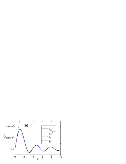
With the resonator amplitude found, we can now go on to calculate the cavity noise. Before doing this, we look at some simple approximations to the damping. In the limit $z\to 0$, we only need include the $n=0,1$ terms in the sum and take the first order in $z$ to get a linear damping,

$$\gamma_{SS}^{z\to 0} = \frac{-x_{s}^{2}\omega_{0}^{2}2\Delta\epsilon_{J}^{2}\Gamma(13\frac{\Gamma^{2}}{4}+\omega_{D}^{2}+\Delta^{2})}{x_{q}^{2}(\Delta^{2}\!+\!\frac{\Gamma^{2}}{4})(\Gamma^{2}\!+\!\omega_{D}^{2})((\Delta^{2}\!+\!\frac{\Gamma^{2}}{4}\!-\!\omega_{D}^{2})^{2}\!+\!\omega_{D}^{2}\Gamma^{2})}$$

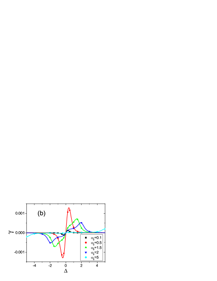
where we note that it is the driving frequency $\omega_{D}$ that appears in the above expression rather than $\omega_{0}$ as the driving field means the periodic motion is at this frequency. In the absence of external driving, $\omega_{D}$ is replaced with $\omega_{0}$ in the above expression. Equation (LABEL:eq:lindamp) then reduces to the previously known effective damping bia ; SSET1 ; bc , but in the limit $\epsilon_{J}\ll\Gamma$ and extending to all resonator frequencies cunpub rather than just $\omega_{0}\ll\Gamma$. In Fig. 3(b), the linear damping is compared to a value obtained numerically from the mean-field equations for a range of values of $\omega_{D}/\Gamma$.

We also find that we can get a relatively simple expression that is exact to $\mathcal{O}(z^{3})$, and valid for finite driving in the limit $\omega_{D}\gg\Gamma$, and for a detuning that is not too large, $|\Delta|\lesssim\omega_{D}$. Including only the $n=-1..2$ terms gives,

$$\gamma_{SS}(z)\approx$$

$$\gamma_{SS}^{z\to 0}\frac{2J_{0}(z)J_{1}(z)}{z}-\frac{4\Delta\epsilon_{J}^{2}x_{s}^{2}J_{1}(z)J_{2}(z)}{x_{q}^{2}z}\times\cdots$$

$$\Re\left\{\frac{(3\Gamma+2i\omega_{D})3i\Gamma\omega_{D}}{(\Gamma\!+\!i\omega_{D})\left((\frac{\Gamma}{2}\!-\!i\omega_{D})^{2}\!+\!\Delta^{2}\right)\left((\frac{\Gamma}{2}\!+\!2i\omega_{D})^{2}\!+\!\Delta^{2}\right)}\right\}$$

This approximation to the amplitude-dependent damping is plotted in Fig. 3(b).

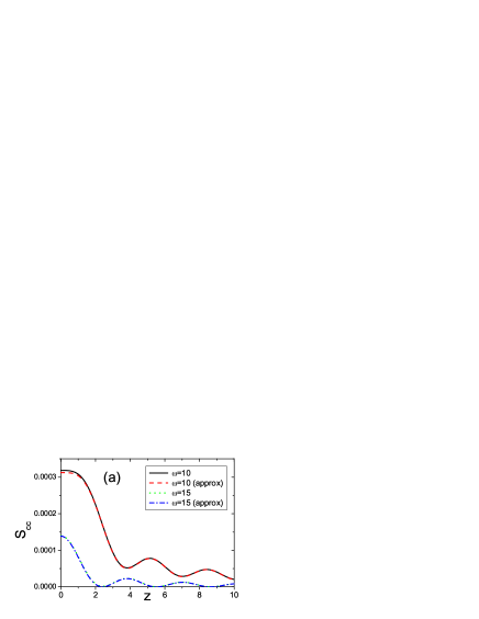
The fluctuations in the charge act as an additional diffusion term for the resonator field Blanter04 . When there is no external driving, we can insert the $z\to 0,\omega_{r}\approx\omega_{0}$ limits of the damping and the charge noise to obtain a simple effective temperature. We find,

$$(2\bar{n}_{SS}+1) = \frac{\frac{\Gamma^{2}}{4}+\Delta^{2}+\omega^{2}}{2\Delta\omega_{0}}$$ (36)

which again agrees with the previously known results bia ; SSET1 ; cunpub for this system. Although this expression has here been derived in the low-$\epsilon_{J}$ limit, other calculations cunpub suggest that this expression is exact for all $\epsilon_{J}$.

Interestingly, this expression for the effective temperature is identical to the expression found when the mechanical resonator is coupled to an optical cavity (or equivalent systems) rather than an SSET Rae ; MCCG ; BlencoweBuks , with the quasiparticle tunneling rate $\Gamma$ simply replaced with the optical cavity damping. This is a rather surprising result, as we have two very different systems, an harmonic oscillator and a 3-level SSET, providing the same effective temperature. The temperature is somehow insensitive to the details of the measuring device - in particular its finite level structure. This merits further investigation, and it would be interesting to see if other related measuring devices also lead to the same expression.

V Sensitive dependence of the sidebands on the driving amplitude

In this section we discuss in detail the rather sensitive dependence of the height of the sideband peaks on the driving amplitude. Due to the Bessel functions, the systematic and noisy response of the charge at the sidebands oscillate rapidly as a function of $z$. We investigate this and suggest that it could be used to detect the presence of small changes in the amplitude of a large driving force.

The power of the systematic peaks in the frequency spectrum is smaller than that in the noisy peaks by a factor of $\epsilon_{J}^{2}$, and decreases as $1/z^{2}$, so we concentrate on the peaks in the spectrum due to the fluctuating terms.

We envision driving the system at some (possibly large) value of $z=z_{0}$. As the heights of the peaks at the sidebands oscillates rapidly as a function of $z=z_{0}+\delta z$, a small change of $\delta z$ will lead to a large change in the height of the sideband peaks.

The sensitivity of the detector depends on the height of the peak at $z_{0}$ compared to the minimum height that the peak can have, i.e. the floor in the frequency spectrum at this point. Equation (25) gives an expression for the heights of the peaks as a function of $z$, and thus we have a simple expression for the ratio,

$$R \approx \frac{4J_{n}(z_{max})^{2}+2J_{0}(z_{max})^{2}}{4J_{n}(z_{min})^{2}+2J_{0}(z_{min})^{2}}$$ (37)

We find this gives a reasonable approximation for odd $n$, and for low values of $z$ when $n$ is even. However, the approximation breaks down when $z$ becomes large. When $z$ is large, the Bessel functions tend to their asymptotic limit $J_{n}(z)\to\frac{2}{\pi z}\cos(z-n\frac{\pi}{2}-\frac{\pi}{4})$, and we find that $J_{n}^{2}=J_{0}^{2}$ for all even $n$, so Eq. (37) diverges at the point where $J_{0}(z_{min})=0$. In this limit, in order to obtain the correct value for the ratio, we need to include terms to the next order in $1/\omega_{D}$.

However, examining Eqs. (21) and (22), we see that all the terms in the sum are of order $1/\omega_{D}^{2}$, i.e. to go to next order requires us to perform an infinite sum. Fortunately, this can be done in the large $z$ limit when the Bessel functions take their asymptotic form.

For example, we can rewrite Eq. (22) at $\omega\approx\omega_{D}n_{e}$, where $n_{e}$ is even and $n_{e}>0$, separating out the odd and even terms to obtain, in the limit $\Gamma,\Delta\ll\omega_{D}$,

$$S_{cc}^{\eta_{02},\eta_{20}}(\omega) \approx \frac{4}{(\omega_{D}n_{e})^{2}}\frac{J_{0}\left(z\right)^{2}\Gamma\epsilon_{J}^{2}/(2\pi)}{\frac{\Gamma^{2}}{4}+\Delta^{2}}$$ (38)

$$+\frac{4}{(\omega_{D}n_{e})^{2}}\sum\limits_{n}\frac{J_{2n}\left(z\right)^{2}\Gamma\epsilon_{J}^{2}/(2\pi)}{(2n\omega_{D})^{2}}$$

$$+\frac{4}{(\omega_{D}n_{e})^{2}}\sum\limits_{n}\frac{J_{2n+1}\left(z\right)^{2}\Gamma\epsilon_{J}^{2}/(2\pi)}{((2n+1)\omega_{D})^{2}}.$$

We now use the fact that in the large $z$ limit, $J_{n}(z)^{2}$ has the same value for all even and all odd $n$. This allows us to perform the sums exactly, using expressions like $\sum\frac{1}{m^{2}}=\frac{\pi^{2}}{6}$ to obtain,

$$S_{cc}^{\eta_{02},\eta_{20}}(\omega) \to \frac{4J_{0}\left(z\right)^{2}\Gamma\epsilon_{J}^{2}}{(\omega_{D}n_{e})^{2}(2\pi)}\left(\frac{1}{\frac{\Gamma^{2}}{4}+\Delta^{2}}+\frac{\pi^{2}}{12\omega_{D}^{2}}\right)$$ (39)

$$+\frac{4J_{1}\left(z\right)^{2}\Gamma\epsilon_{J}^{2}}{(\omega_{D}n_{e})^{2}(2\pi)}\left(\frac{\pi^{2}}{4\omega_{D}^{2}}\right).$$

Performing similar calculations for Eqs. (21) and (III.2) gives asymptotic forms for the charge noise for at the odd, even and zeroth peak to leading order,

$$S_{cc}(0) \to \frac{\epsilon_{J}^{2}}{\pi z\Gamma}\frac{13\Gamma^{2}+4\Delta^{2}}{(\frac{\Gamma^{2}}{4}+\Delta^{2})^{2}}\cos^{2}(z-\frac{\pi}{4})+\frac{\pi\epsilon_{J}^{2}}{z\omega_{D}^{2}\Gamma}$$

$$S_{cc}(n_{e}) \to \frac{\epsilon_{J}^{2}\Gamma}{n_{e}^{2}\omega_{D}^{2}\pi z}\frac{12}{\frac{\Gamma^{2}}{4}+\Delta^{2}}\cos^{2}(z-\frac{\pi}{4})+\frac{3\pi\Gamma\epsilon_{J}^{2}}{z\omega_{D}^{4}n_{e}^{2}}$$

$$S_{cc}(n_{o}) \to \frac{\epsilon_{J}^{2}\Gamma}{n_{o}^{2}\omega_{D}^{2}\pi z}\frac{4}{\frac{\Gamma^{2}}{4}+\Delta^{2}}(1+\sin^{2}(z-\frac{\pi}{4})).$$ (40)

The odd peaks have a ratio between maximum and minimum of order one, so will not be of as much use. The even peaks have maxima at $z=m\pi+\frac{\pi}{4}$, minima at $z=m\pi+\frac{3\pi}{4}$, and are most sensitive to changes in $z$ at $z=\frac{m\pi}{2}$. The ratio between the height of the peaks at their maxima and at their minima takes a simple form when $n>0$. We find,

$$R_{n_{e}>0}=\frac{\omega_{D}^{2}}{\frac{\Gamma^{2}}{4}+\Delta^{2}}$$ (41)

so the contrast between the peaks at their largest and smallest can become large in the limit $\omega_{D}\gg\Gamma,\Delta$.

VI Cavity Output Field

In this section we describe how the noise spectrum of the field in the cavity is transferred to the quantities that are actually measured. In order to connect the dynamics of the resonator to measured quantities we need to consider how the resonator is coupled to the external world. What form this takes depends on what the resonator actually is. For example, if it is the microwave field in a superconducting co planar cavity, we can use the input-output formalism of quantum optics to relate the field in the microwave cavity to the many mode fields in transmission lines connected to the cavity. In this situation, the damping and noise on the resonator is attributed to fields external to the cavity and these external fields are ultimately what is measured. In the simplest situation we could imagine a single side cavity with a quantum limited input field. The output field from the cavity then contains a component of the reflected input field as well as the field transmitted from the cavity itself. This is the model we will adopt here as we can easily apply the input-output theory of quantum optics WM as co-planar superconducting cavities are in the highly underdamped limit appropriate for this formalism.

Another possible realization for the resonator is a nanomechanical oscillator. In this case, we need an explicit transducer model for the way in which the displacement of the nanomechanical resonator is measured. A typical example would be to capacitively couple the nanomechanical resonator to a microwave cavity WoolleyMilb . In that case the nanomechanical resonator is coupled to more than one bath: the finite-temperature mechanical bath in addition to its irreversible coupling to the microwave field propagating into and out of the transducer cavity. For a fast and efficient measurement, the microwave cavity would be strongly damped in which case the resonator would see the bosonic bath due to the electromagnetic fields on the transmission lines directly.

The quantum Langevin equation for the field is given in Eq. (5). In the microwave realization, we will assume a single side cavity and that the only source of damping for the cavity field is in fact its coupling to the input and output fields at the open end of the cavity. In that case the noise operator, $\eta_{a}$ is written in terms of the multi-mode field amplitude input to the cavity: $\eta_{a}(t)=\sqrt{\gamma_{ex}}a_{in}(t)$. The output field from the cavity is related to the input field and the intracavity field by

$$a_{o}(t)=\sqrt{\gamma_{ex}}a(t)-a_{in}(t)$$ (42)

In terms of the Fourier transformed operators, the input and output fields are related by

$$a_{o}(\omega) = -\frac{i\sqrt{\gamma_{ex}}A_{D}\delta(\omega+\omega_{D})}{\frac{\gamma_{ex}}{2}+i(\omega_{D}+\omega)}+\frac{i\sqrt{\gamma_{ex}}\chi\sigma_{cc}(\omega)}{\frac{\gamma_{ex}}{2}+i(\omega_{D}+\omega)}$$ (43)

$$+\frac{\frac{\gamma_{ex}}{2}-i(\omega_{D}+\omega)}{\frac{\gamma_{ex}}{2}+i(\omega_{D}+\omega)}a_{in}(\omega)$$

where the last term represents a phase shift between incident and reflected field components from a single-sided cavity, and

$$\chi=\frac{\omega x_{s}}{2x_{q}}$$ (44)

and $\sigma_{cc}(\omega)$ is the Fourier transform of the island charge operator $\sigma_{cc}(t)$. In general this is itself a function of the intracavity field and so $\sigma_{cc}(\omega)$ is a complicated convolution of a very nonlinear operator-valued function of $a(\omega)$ and thus Eq.(43) is not an explicit relation between the input and output field components. However if we adopt the approximation implicit in Eq. (LABEL:eq:resnoisenba), we can write it in terms of a systematic component and noise component as

$$a_{o}(\omega) = -\frac{i\sqrt{\gamma_{ex}}A_{D}\delta(\omega+\omega_{D})}{\frac{\gamma_{ex}}{2}+i(\omega_{D}+\omega)}+\frac{i\sqrt{\gamma_{ex}}\chi\sigma^{S}_{cc}(\omega)}{\frac{\gamma_{ex}}{2}+i(\omega_{D}+\omega)}$$

$$+\frac{i\sqrt{\gamma_{ex}}\chi\sigma^{\eta}_{cc}(\omega)}{\frac{\gamma_{ex}}{2}+i(\omega_{D}+\omega)}+\frac{\frac{\gamma_{ex}}{2}-i(\omega_{D}+\omega)}{\frac{\gamma_{ex}}{2}+i(\omega_{D}+\omega)}a_{in}(\omega)$$

We thus see that the noise power spectrum for the field output from the cavity is

$$S_{out}(\omega) = \int_{-\infty}^{\infty}d\omega^{\prime}\langle a_{o}^{\dagger}(\omega),a_{o}(\omega^{\prime})\rangle$$ (46)

$$= \bar{n}(\omega)+\frac{\chi^{2}(S_{c,c}^{S}(\omega)+S^{\eta}_{c,c}(\omega))}{(\omega-\omega_{0})^{2}+\frac{\gamma_{ex}^{2}}{4}}$$

and we see that, for small enough $\bar{n}$, the noise of the cavity is transferred to the output field, and thus the emitted field can be used to detect the noise in the cavity.

VII Conclusion

We have used a Langevin equation approach to investigate the frequency spectrum of a superconducting single electron transistor coupled to a resonator under periodic driving of the resonator. The fluctuating noise terms allow us to describe the correlations in the SSET due to the finite level structure. This approach allows the calculation of the spectrum of the charge noise in the SSET and the resulting effect on the resonator field in the limit of low Josephson energy, $\epsilon_{J}\ll\Gamma$. We found that the charge noise consists of a series of peaks at multiples of the driving frequency, and calculated the heights at and between these noise peaks in the limit of fast resonator oscillation.

We have calculated the effect of the SSET on the cavity, and in particular calculated an effective amplitude-dependent damping and temperature that is valid for all resonator frequencies. We have shown that the peaks at the sidebands depend rather sensitively on the driving amplitude and show how this could provide a measure of small changes in the driving amplitude.

We thank Andrew Armour and Thomas Harvey for helpful discussions. D.A. Rodrigues acknowledges funding under EPSRC grant EP/D066417/1.

Appendix A Derivation of the Langevin equations

In this appendix we describe in more detail our use of the Langevin equations and show how they can be derived from the master equation. We show that this approach reproduces the results obtained by other methods for an SSET uncoupled to a resonator.

We assume that the noise in the system is entirely determined by the second order correlation functions for the dynamical variables. We find that we can use Langevin equations as a useful tool for keeping track of the dynamics of the first and second moments. If the Langevin equations give the same equations of motion for the first two moments as a master equation or Focker-Planck equation then, as far as a noise calculation is concerned, the two are equivalent. This equivalence is discussed in Ref. WM , and a description of a noise calculation given for the case when the conservative terms and the diffusion in the Langevin equation are constant in time. Here we focus on the situation where the external driving means that these terms are time-dependent.

Although Langevin equations can be derived from a microscopic picture, in which the noise terms $\eta(t)$ represent the correlation functions of the external bath (in this case the microscopic electron energy levels in the leads) here we take a functional approach and consider them simply as a tool to allow us to describe the correlation functions of the system. In this approach we find that we can derive the properties of the noise operators from the master equation. A general set of Langevin equations $\bar{x}(t)$ with systematic evolution described by the matrix $A(t)$ and fluctuations $\bar{E}(t)$ gives,

$$\dot{\bar{x}}(t) = -A(t)\bar{x}+\bar{E}(t)$$ (47)

$$\bar{x}(t) = \bar{x}(0)e^{-I(t)}+e^{-I(t)}\int\limits_{0}^{t}e^{I(t^{\prime})}\bar{E}(t^{\prime}){\textrm{d}}t^{\prime}$$ (48)

where $I(t)=\int\limits_{0}^{t}A(t^{\prime}){\textrm{d}}t$. From Eq. (47) we can calculate equation of motion for the variance $\chi(t)=\bar{x}(t)\bar{x}^{T}(t)$,

$$\dot{\chi}(t) = \bar{x}(t)\left(-\bar{x}^{T}(t)A^{T}(t)+\bar{E}^{T}(t)\right)$$ (49)

$$+\left(-A(t)\bar{x}(t)+\bar{E}(t)\right)\bar{x}^{T}(t)$$

Inserting Eq. (48) and taking the ensemble average gives,

$${\left\langle\dot{\chi}(t)\right\rangle} = -(A(t){\left\langle\chi(t)\right\rangle}+{\left\langle\chi(t)\right\rangle}A^{T}(t))$$ (50)

$$+\left\langle\bar{E}(t)\left(\int\limits_{0}^{t}\bar{E}^{T}(t^{\prime})e^{I^{T}(t^{\prime})}{\textrm{d}}t^{\prime}\right)e^{-I^{T}(t)}\right\rangle$$

$$+\left\langle\left(e^{-I(t)}\int\limits_{0}^{t}e^{I(t^{\prime})}\bar{E}(t^{\prime}){\textrm{d}}t^{\prime}\right)\bar{E}^{T}(t)\right\rangle$$

If the dynamics of the system is Markovian (as in our master equation), the fluctuating noise correlators will be $\delta$-correlated. Indeed, a microscopic derivation shows that $\delta$-correlated operators are obtained in exactly the limit that the master equation becomes Markovian, i.e. when the decay of the correlation functions of the leads is much more rapid than any timescale in the system.

Writing the correlation matrix of the noise terms as ${\left\langle\bar{E}(t)\bar{E}^{T}(t^{\prime})\right\rangle}=\delta(t-t^{\prime})G(t)$, we obtain an expression that relates the rate of change of the variance matrix to the Langevin correlators,

$${\left\langle\dot{\chi}(t)\right\rangle} = -(A(t){\left\langle\chi(t)\right\rangle}+{\left\langle\chi(t)\right\rangle}A^{T}(t))+G(t)$$ (51)

which reduces to the usual WM $A{\left\langle\chi\right\rangle}+{\left\langle\chi\right\rangle}A^{T}=G$ for the case of a time-independent $A$. The fluctuations represent deviations from the mean field so we can also calculate $\mathbf{G}$ by comparing the true evolution of the second moments with the mean-field-only evolution, which is sometimes more convenient in practice. Defining $\dot{\bar{\varsigma}}=-\mathbf{A}\bar{x}$, the elements of $\mathbf{G}$ are also given by,

$${G_{ij}}=\dot{{\left\langle x_{i}x_{j}\right\rangle}}-{\left\langle\dot{\varsigma_{i}}x_{j}\right\rangle}-{\left\langle x_{i}\dot{\varsigma_{j}}\right\rangle}.$$ (52)

Using either Eq. 51 or Eq. 52, we find that the correlators for the SSET are given by,

$$G_{00,00} = -G_{00,11}=-G_{11,00}=\Gamma{\left\langle\sigma_{11}(t)\right\rangle}$$

$$G_{22,22} = -G_{11,22}=-G_{22,11}=\Gamma{\left\langle\sigma_{22}(t)\right\rangle}$$

$$G_{02,22} = -G_{02,11}=\Gamma{\left\langle\sigma_{02}(t)\right\rangle}$$

$$G_{22,20} = -G_{11,20}=\Gamma{\left\langle\sigma_{20}(t)\right\rangle}$$

$$G_{11,11} = \Gamma({\left\langle\sigma_{11}(t)\right\rangle}+{\left\langle\sigma_{22}(t)\right\rangle})$$

$$G_{02,20} = \Gamma({\left\langle\sigma_{00}(t)\right\rangle}+{\left\langle\sigma_{11}(t)\right\rangle}),$$ (53)

with all other correlators equal to zero. We note that the commutation relations are preserved, e.g. $G_{02,22}\neq G_{22,02}$, retaining the quantum nature of the problem. It is also worth re-emphasizing that this functional approach where we derive the correlators through the equations of motion for the variance means that we are only capturing 2nd-order correlations. This is adequate for our purposes, as the noise only requires these terms, but these Langevin equations give no information about higher-order correlations.

We can check the validity of this approach to deriving the Langevin correlators in a simple case where the noise can be calculated by other methods. For the case of an undriven, uncoupled SSET, inserting the Fourier transforms of Eqs. (6) to (I) along with the expressions for the correlators from Eq. (53) in the expression for the noise, Eq. (14), gives an expression that is mathematically identical to the noise as calculated more directly using the expression

$${\left\langle\sigma_{ij}(t+\tau)\sigma_{kl}(t)\right\rangle}={\left\langle\exp(-A\tau)\sigma_{ij}(t)\sigma_{kl}(t)\right\rangle}$$ (54)

which can be evaluated by exactly diagonalizing $A$. In particular, this is true for all values of $\Gamma$ compared to the other SSET timescales, $\Delta,\epsilon_{J}$. We can also use the converse of this argument to confirm that the noise terms must indeed be $\delta-$correlated.

References

- (1) Y. Nakamura, Yu. A. Pashkin and J. S. Tsai, Nature 398 786 (1999)
- (2) J. M. Martinis, S. Nam, J. Aumentado and C. Urbina, Phys. Rev. Lett. 89 117901 (2002)
- (3) A. Cottet, D. Vion, P. Joyez, P. Aassime, D. Esteve and M. H. Devoret, Physica C 367 197 (2002)
- (4) J. E. Mooij, T. P. Orlando, L. Levitov, L. Tian, C. H. van der Wal, and S. Lloyd, Science 285 1869 (1999)
- (5) A. Blais, R.-S. Huang, A. Wallraff, S. M. Girvin, and R. J. Schoelkopf, Phys. Rev. A 69 062320 (2004); A. Wallraff, D. I. Schuster, A. Blais, L. Frunzio, R.-S. Huang, J. Majer, S. Kumar, S. M. Girvin and R. J. Schoelkopf Nature 431 162 (2004)
- (6) M. P. Blencowe, Phys. Rep. 395 159 (2004)
- (7) D. Mozyrsky and I. Martin Phys. Rev. Lett. 89 018301 (2002)
- (8) A. A. Clerk and S. M. Girvin Phys. Rev. B 70 121303(R) (2004)
- (9) J. Wabnig, D. V. Khomitsky, J. Rammer and A. L. Shelankov Phys. Rev. B 72 165347 (2005)
- (10) D. Mozyrsky, I. Martin and M. B. Hastings Phys. Rev. Lett. 92 018303 (2004)
- (11) A. D. Armour, M. P. Blencowe and Y. Zhang Phys. Rev. B 69 125313 (2004)
- (12) R. S. Knobel, and A. N. Cleland Nature 424 291 (2003)
- (13) D. A. Rodrigues and A. D. Armour New. J. Phys. 7 251 (2005).
- (14) D. A. Rodrigues, J. Imbers and A. D. Armour Phys. Rev. Lett. 98 067204 (2007)
- (15) D. A. Rodrigues, J. Imbers, T. J. Harvey and A. D. Armour New. J. Phys. 9 84 (2007).
- (16) M. P. Blencowe, J. Imbers and A. D. Armour New J. Phys. 7 236 (2005)
- (17) A. A. Clerk and S. D. Bennett New J. Phys. 7 238 (2005)
- (18) S. D. Bennett and A. A. Clerk Phys. Rev. B 74, 201301(R) (2006)
- (19) M. D. LaHaye, O. Buu, B. Camarota and K. C. Schwab Science 304 74 (2004)
- (20) A. Naik, O. Buu, M. D. LaHaye, A. D. Armour, A. A. Clerk, M. P. Blencowe and K. C. Schwab, Nature 443, 193 (2006)
- (21) P. Filipowicz, J. Javanainen and P. Meystre, Phys. Rev. A 34, 3077 (1986).
- (22) H. Walther, B. T. H. Varcoe, B.-G. Englert, and T. Becker, Rep. Prog. Phys. 69 1325 (2006)
- (23) O. Astafiev, K. Inomata, A. O. Niskanen, T. Yamamoto, Yu. A. Pashkin, Y. Nakamura, and J. S. Tsai, Nature 449 588 (2007).
- (24) M.-S. Choi, R. Fazio, J. Siewert, and C. Bruder, Europhys. Lett. 53 251 (2001); M.-S. Choi, F. Plastina and R. Fazio Phys. Rev. B 67 045105 (2003)
- (25) A. A. Clerk, S. M. Girvin, A. K. Nguyen, and A. D. Stone Phys. Rev. Lett. 89 176804 (2002)
- (26) J. Hauss, A. Fedorov, C. Hutter, A. Shnirman and G. Schön Phys. Rev. Lett. 100 037003 (2008)
- (27) A. A. Clerk Phys. Rev. B 70 245306 (2004)
- (28) F. Marquardt, J. G. E. Harris and S. M. Girvin Phys. Rev. Lett. 96 103901 (2006)
- (29) M. Ludwig, B. Kubala and F. Marquardt arXiv:0803.3714 (2008)
- (30) Ya. M. Blanter, O. Usmani and Yu. V. Nazarov, Phys. Rev. Lett. 93 136802 (2004); ibid., Phys. Rev. Lett. (erratum) 94 0409904 (2005)
- (31) A. A. Clerk, unpublished; D. A. Rodrigues, unpublished
- (32) I. Wilson-Rae, N. Nooshi, W. Zwerger and T. J. Kippenberg Phys. Rev. Lett. 99 093901 (2007)
- (33) F. Marquardt, J. P. Chen, A. A. Clerk and S. M. Girvin Phys. Rev. Lett. 99 093902 (2007)
- (34) M. P. Blencowe and E. Buks Phys. Rev. B 76 014511 (2007)
- (35) D. F. Walls and G. J. Milburn, Quantum Optics (Berlin: Springer-Verlag) (1994)
- (36) M. J. Woolley, A. C. Doherty, G. J. Milburn, K. C. Schwab, arXiv:0803.1757 (2008).
- (37) C. B. Doiron, B. Trauzettel and C. Bruder, Phys. Rev. B 76 195312 (2007)