Phase transition of Two-timescale Two-temperature Spin-lattice Gas Model

Abstract

We study phase transition of a nonequilibrium statistical-mechanical model, in which two degrees of freedom with different time scales separated from each other touch to their own heat bath. A general condition for finding anomalous negative latent heat recently discovered is derived a from thermodynamic argument. As a specific example, phase diagram of a spin-lattice gas model is studied based on a mean-field analysis with replica method. While configurational variables are spin and particle in this model, it is found that the negative latent heat appears in a parameter region of the model, irrespective of the order of their time scale. Qualitative differences in the phase diagram are also discussed.

I introduction

Phase transitions under non-equilibrium conditions have attracted with a great deal of attention in statistical-mechanical problemsNEPT ; NEPT2 ; NEPT3 . There have been many investigations on non-equilibrium phase transitions so farDRIVEN ; SHEAR ; R ; ZPM , which have revealed a fascinating new transition behavior different from equilibrium transition. In general, probability distribution in non-equilibrium cannot be expressed in terms of only energy functional, which causes a difficulty in theoretical study.

Recently another class of non-equilibrium systems that exhibits a phase transition has been studiedAP , in which two different degrees of freedom coupled to their own heat baths interact with each other through multi-body interactions. For simplicity, time scales of these two variables are assumed to be well separated. Then, the systems consist of slow and fast variables belonging to different time hierarchy. The fast variables behave in quasi-equilibrium for a given set of slow variables that plays a role as quenched variables for the fast ones. Meanwhile, the slow variables are not given by independent distribution function as in quenched disordered systems but affected through mean force of fluctuating fast variables. Such systems with a hierarchy in seperated time scales and different heat baths are here called “two-temperature” system. These systems are adopted to describe neural network systems with a synaptic evolutionCPS , evolving networksWS , and some kind of NMR systemsDFK . In contrast to most of non-equilibrium systems, the steady-state distribution of the models is formally expressed in terms of the energy function using the replica method that is a standard tool for studying thermodynamic properties of the quenched disordered systemsMPV .

The replica formalism for two-temperature systems has been introduced in Refs. [CPS, ; Dotsenko, ; ANS, ]. While the quenched disordered systems require the replica limit in which the replica number takes to be zero, the two-temperature systems have a physical meaning for any value of the replica number which corresponds to a ratio of two temperatures. In this sense, this is regarded as a generalization of quenched systems and is sometimes called as partial annealing systemCPS . A most crutial difference from the quenched systems is that the slow variables are also dynamical coupled to their heat bath. Therefore, both the slow and fast variables are responsible for phase transition. This could provide a new cooperative phenomenon over different time scale.

In fact, Allahverdyan and Petrosyan, hereafter referred to as AP, studied a mean-field spin model as a two-temperature system and found that the model exhibited a first-order phase transition with anomalous negative latent heat, which never occurs in equilibrium statistical mechanics. However, this peculiar behavior observed in the two-temperature system is not well understood. We pursue phase transition in the two-temperature systems and give a general condition that the system exhibits the negative latent heat with the help of the idea of thermodynamics. It is also found that, in the systems, two different entropys associated with the fast and slow variables respectively play a competitive role in determing the phase boundary of first-order transition. We further studied two-temprature version of a spin-lattice-gas model, similar to that studied by AP, as a specific example. The spin-lattice-gas model consists of two degrees of freedom, spins and particles, which has been studied for a given Hamiltonian in equilibriumSok . The two-temperature version is characterized by not only the Hamiltonian but also the order of time scales of two variables. AP studied the case where the spins were slow and the particles were fast. We study this case with some modified Hamiltonian and also the other case, namely the spins and particles behave as fast and slow variables, respectively. We then find that the existence of the negative latent heat is common to both cases, suggesting that it is observed in a wide class of the two-temperature systems. On the other hand, qualitatively different behavior is also found in phase diagram of the two cases, in particluar, the stability of ferromagnetic ordered phase.

This paper is organized as follows. In Sec. II, we review the replica formalism of the two-temperature system, which leads to an equilibrium model of a replicated system. We also discuss phase boundary of first-order transition and derive a Clausius-Clapeyron relation in this system. This relation enables us to find generally a geometric property of the phase boundary and the negative latent heat. In Sec. III, we explicitly define two mean-field spin-lattice-gas models with different order of time scales and give self-consistent equations for the models. The results obtained by solving the equations are presented in Sec. IV. In Sec. V, we summarize our results.

II Two-temperature formalism with different time scales

In this section, we review a theoretical formalism for two-time-scale and two-temperature systemAP . Suppose a system described by a Hamiltonian $H(f,s)$, in which $f$ is a symbolic notation of fast degree of freedom and $s$ is of slow degree of freedom. These variables $f$ and $s$ are in contact with their different heat bath with temperature $T_{f}$ and $T_{s}$, respectively. We assume that the two characteristic time scales on the variables $s$ and $f$ are well separated from each other and that the thermal average of the fast variable $f$ can be taken with a fixed configuration of the slow variable $s$. Then, the conditional probability $P(f|s)$ of finding a configuration $f$ for a given $s$ at the inverse temperature $\beta_{f}=1/T_{f}$ is defined

$$P(f|s)=\frac{e^{-\beta_{f}H(f,s)}}{Z(s)},$$ (1)

where the normalization constant or the partition function of the fast variable is set as

$$Z(s)=\mathrm{Tr}_{f}e^{-\beta_{f}H(f,s)}.$$ (2)

Hereafter the Boltzmann constant is set to be unity. One can define partial free energy for the fast variable as $F_{f}(s)=-T_{f}\log{Z}(s)$.

The steady-state probability of slow variables $P(s)$ is derived by an adiabatic approximation of two-temperature Langevin equation ANS . The force acting on $s$ is assumed to be an averaged derivative of the Hamiltonian with respect to the slow variable over the conditional probability, which is represented by the partial free energy as $-\frac{\partial F_{f}(s)}{\partial s}$. The equilibrium distribution $P(s)$ at the inverse temperature $\beta_{s}=1/T_{s}$ is given by

$$P(s) = \frac{e^{-\beta_{s}F_{f}(s)}}{\mathcal{Z}}$$ (3)

where

$$\mathcal{Z} = \mathrm{Tr}_{s}e^{-\beta_{s}F_{f}(s)}.$$ (4)

The total free energy $\mathcal{F}$ is defined by $\mathcal{F}=-T_{s}\log{\mathcal{Z}}$.

Using the replica trick, the model can be mapped onto an equilibrium problem with a replicated Hamiltonian for the integer number of ratio $n=T_{f}/T_{s}$,

$$\mathcal{F} = -T_{s}\log\left(\mathrm{Tr}_{s}\mathrm{Tr}_{f}^{(1)}\cdots\mathrm{Tr}_{f}^{(n)}e^{-\beta_{f}\sum_{l=1}^{n}H(f^{(l)},s)}\right),$$ (5)

where $f^{(l)}$ denotes replicated fast variables. This could be extended to any real value of the ratio $T_{f}/T_{s}$ after calculating the replicated system in a standard manner of the replica method. While one takes the replica limit $n\rightarrow 0$ for the quenched disordered system like spin glasses, any value of $n$ makes a sense as the two-temperature system in this context. This formalism is also interpreted as a kind of statistical-mechanical problems with randomness. In particular, note that the distribution of the random variables is determined by not only a given independent function but also the thermal averaged quantity of the fast variables. The latter leads to a non-trivial correlation among the slow variables.

We discuss thermodynamic properties of the two-temperature system. The simultaneous probability $P(f,s)$ is expressed as $P(f,s)=P(f|s)P(s)$. The total entropy $S$ defined by the simultaneous probability is decomposed into two degrees of freedom as

$$S=-\mathrm{Tr}_{s,f}P(f,s)\log P(f,s)=\mathcal{S}_{s}+S_{f},$$ (6)

where $S_{s}$ and $S_{f}$ are expressed as

$$\mathcal{S}_{s} = -\mathrm{Tr}_{s}P(s)\log P(s),$$ (7)

$$S_{f} = -\mathrm{Tr}_{s}P(s)\left(\mathrm{Tr}_{f}P(f|s)\log P(f|s)\right).$$ (8)

The total free energy $\mathcal{F}$ is formally expressed as

$$\mathcal{F}(T_{s},T_{f})=\overline{\langle H(f,s)\rangle_{f}}-T_{f}S_{f}-T_{s}\mathcal{S}_{s},$$ (9)

where $\langle\cdots\rangle_{f}$ and $\overline{\cdots}$ denote an average over the variables $f$ with $P(f|s)$ and $s$ with $P(s)$, respectively. It should be noted that the free energy is also rewritten by

$$\mathcal{F}(T_{s},T_{f})=\overline{F_{f}(s)}-T_{s}\mathcal{S}_{s}.$$ (10)

Averaging over the fast variables $f$, the thermodynamic structure is found by regarding the averaged partial free energy $\overline{F_{f}(s)}$ as an “energy” for the slow variable $s$. Namely, the averaged partial free energy and the entropy $\mathcal{S}_{f}$ for the slow variables decrease monotonically with decreasing $T_{s}$.

As a consequence of the thermodynamic structureEF , a Clausius-Clapeyron like relation for two-temperature systems is derived, which gives us a topological property of a first-order-transition line. Suppose a phase diagram of the system onto two-temperature plane of $T_{s}$ and $T_{f}$. We take two points $(T_{f},T_{s})$ and $(T_{f}+\delta T_{f},T_{s}+\delta T_{s})$ which are located on either side of the first-order-transition line. The free-energy difference $\delta F$ between these points with small temperature differences $\delta T_{f}$ and $\delta T_{s}$ is given by

$$\delta\mathcal{F}=-S_{f}\delta T_{f}-\mathcal{S}_{s}\delta T_{s}.$$ (11)

At the first-order transition point $(T_{f}^{(1)},T_{s}^{(1)})$, the ordered and disordered states coexist and the free energy of these states coincides with each other, meaning

$$\Delta\mathcal{F}=\mathcal{F}^{(o)}(T_{f}^{(1)},T_{s}^{(1)})-\mathcal{F}^{(d)}(T_{f}^{(1)},T_{s}^{(1)})=0,$$ (12)

where the upper suffixes $o$ and $d$ denote the ordered and the disordered states, respectively, and $\Delta A$ means the difference of a physical quantity $A$ between the ordered and disordered states at the transition point. Using Eqs. (11) and (12), the Clausius-ClapeyronEF like relation is obtained as

$$\frac{\delta T_{s}^{(1)}}{\delta T_{f}^{(1)}}=-\frac{\Delta S_{f}}{\Delta\mathcal{S}_{s}}.$$ (13)

This implies that when the slope of the phase boudary $dT_{s}^{(1)}/dT_{f}^{(1)}$ is positive, $\Delta\mathcal{S}_{s}$ and $\Delta S_{f}$ are opposite to each other. The free-energy difference $\Delta\mathcal{F}$ is also expressed as $\Delta\mathcal{F}=\Delta\mathcal{U}-T_{f}\Delta S_{f}-T_{s}\Delta\mathcal{S}_{s}$ with $\mathcal{U}$ being the internal energy $\overline{\langle H\rangle_{f}}$. Thus, we obtain the relation between the deference of the internal energy and the phase boundary as

$$\Delta\mathcal{U}(T_{f}^{(1)},T_{s}^{(1)})=T_{s}^{(1)}\Delta\mathcal{S}_{s}\left(1-n\frac{dT_{s}^{(1)}}{dT_{f}^{(1)}}\right).$$ (14)

Because the entropy $\mathcal{S}_{s}$ is a monotonically decreasing function of $T_{s}$, the sign of $\Delta\mathcal{U}$ depends on only the gradient of the phase boundary. This implies that the condition to find the negative latent heat is $\frac{1}{n}\leq dT_{s}^{(1)}/dT_{f}^{(1)}$ when $T_{s}$ decreases. On the other hand, when $T_{f}$ decreases, the condition for the negative latent heat changes to $0\leq dT_{s}^{(1)}/dT_{f}^{(1)}\leq\frac{1}{n}$. While AP explicitly found that a specific spin-lattice gas model exhibited the negative latent heat in a region of the phase diagram using the replica method, we find a general condition for which the negative latent heat appears thorough the thermodynamic argument.

III Mean-field spin-lattice gas model

A model Hamiltonian we studied is an infinite-range spin-lattice-gas model, that is given by

$$H(\{S_{i},p_{i}\})=-\frac{1}{N}\sum_{(ij)}\Big{(}JS_{i}S_{j}+\epsilon_{f}\Big{)}p_{i}p_{j}+\alpha\sum_{i=1}^{N}p_{i}$$ (15)

where $S_{i}=\pm 1$ are spin variables, $p_{i}=0,1$ are particle occupation variables and they are defined on $N$ sites. In the case where the spins $S_{i}$ are the slow variable and the particles $\rho_{i}$ the fast, referred to as case-1 model, the model system with $\epsilon_{f}=0$ is identical with that studied by APAP . We also consider the inverse case where the spins and the particles represent the fast and slow variables, respectively, which is referred to as case-2 model. The spin and particle variables are coupled to their own heat baths whose temperature is denoted by $T_{S}$ and $T_{p}$, respectively. The sum is taken over all pairs of sites. The interactions $J$ and $\epsilon_{f}$ denote a ferromagnetic coupling and an attractive interaction between particles, respectively. In this paper, $J$ is taken as a unit of energy and temperature. The first term of the Hamiltonian consists of a spin mediated interaction and direct one. The second term plays a role for controlling a particle number with chemical potential $\alpha$ which is chosen to be a positive value. The spin-lattice-gas model could exhibit two types of phase transition which are magnetic and density orderings. The interaction $-\Big{(}JS_{i}S_{j}+\epsilon_{f}\Big{)}$ between particles prefers to increase the particle density and magnetically ferromagnetic ordering, while the chemical potential $\alpha$ tends to decrease the particle density. In this sense, these two energy terms compete with each other. Furthermore, two different kinds of the entropy associated with the fast and slow variables also compete with the energy terms.

Since the Hamiltonian is an infinite range model, the trace of Eq. (5) is carried out with the help of the replica method by introducing two auxiliary fields $m$ and $\rho$, which correspond to average magnetization and particle density, respectively. The self-consistent equations for $m$ and $\rho$ are written as, for the case-1 model,

$$m = \frac{\displaystyle\sum_{S=\pm 1}S\phi(S;m,\rho)\left(1+\phi(S;m,\rho)\right)^{n-1}}{\displaystyle\sum_{S=\pm 1}\left(1+\phi(S;m,\rho)\right)^{n}},$$ (16)

$$\rho = \frac{\displaystyle\sum_{S=\pm 1}\phi(S;m,\rho)\left(1+\phi(S;m,\rho)\right)^{n-1}}{\displaystyle\sum_{S=\pm 1}\left(1+\phi(S;m,\rho)\right)^{n}},$$ (17)

and for the case-2 model,

$$m = \frac{\Big{(}\displaystyle\sum_{S=\pm 1}S\phi(S;m,\rho)\Big{)}\Big{(}\displaystyle\sum_{S=\pm 1}\phi(S;m,\rho)\Big{)}^{n-1}}{2^{n}+\Big{(}\displaystyle\sum_{S=\pm 1}\phi(S;m,\rho)\Big{)}^{n}},$$ (18)

$$\rho = \frac{\Big{(}\displaystyle\sum_{S=\pm 1}\phi(S;m,\rho)\Big{)}^{n}}{2^{n}+\Big{(}\displaystyle\sum_{S=\pm 1}\phi(S;m,\rho)\Big{)}^{n}},$$ (19)

where $\phi(S;m,\rho)=e^{-\beta_{f}\Big{(}\alpha-mJS-\epsilon_{f}\rho\Big{)}}$. Here $\beta_{f}$ is the inverse of the fast temperature, which corresponds to $1/T_{p}$ in the case-1 model and $1/T_{S}$ in the case-2 model. The free energy of system is represented with a solution $(m_{0},\rho_{0})$ of the above self-consistent equations as

$$\mathcal{F}_{1}(m_{0},\rho_{0},T_{S},T_{p}) = \frac{1}{2}\Big{(}Jm_{0}^{2}+\epsilon_{f}\rho_{0}^{2}\Big{)}$$

$$\qquad\qquad-T_{S}\log\left(\sum_{S=\pm 1}\left(1+\phi(S;m_{0},\rho_{0})\right)^{n}\right)$$ (20)

for the case 1 and

$$\mathcal{F}_{2}(m_{0},\rho_{0},T_{S},T_{p})=\frac{1}{2}\Big{(}Jm_{0}^{2}+\epsilon_{f}\rho_{0}^{2}\Big{)}$$

$$\qquad\qquad-T_{p}\log\Bigg{(}2^{n}+(\ \sum_{S=\pm 1}\phi(S;m_{0},\rho_{0})\ )^{n}\Bigg{)}$$ (21)

for the case-2. Here $n$ is defined as the ratio of the fast temperature to the slow one, namely $n$ is $\frac{T_{p}}{T_{S}}$ and $\frac{T_{S}}{T_{p}}$ for the case-1 and case-2, respectively. In this paper, $\mathcal{F}_{1}$ and $\mathcal{F}_{2}$ as functions of $m$ and $\rho$ are loosely called to “free energy” in a sense of Ginzburg-Landau free energy. According to the Eqs. (7) and (8), two kinds of decomposed entropy are termed as $S_{S}$ and $\mathcal{S}_{p}$, respectively for the case-1 model, and $S_{p}$ and $\mathcal{S}_{S}$ for the case-2 model.

IV Results and discussions

IV.1 Phase diagram and negative latent heat

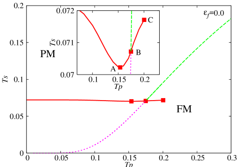
art

Figure 1: Phase diagram of the case-2 model on $T_{S}-T_{p}$ plane with $\alpha=0.45$ and $\epsilon_{f}=0$. PM and FM denote paramagnetic and ferromagnetic phases, respectively. The solid and dashed lines represent the first and second order transitions and the dotted one represents the instability limit of the paramagnetic solution. The inset shows an enlarged view around the critical point.

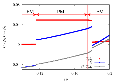
Figure 2: $T_{p}$ dependence of $\mathcal{U}$, $T_{S}\mathcal{S}_{S}$, and averaged partial free energy $\overline{F_{S}(p)}=\mathcal{U}-T_{S}\mathcal{S}_{S}$ at $\alpha=0.45$ and $T_{S}=0.071$ in the case-2 model. There are three phase transitions, indicated by vertical lines, with $T_{p}$ changing for a fixed $T_{S}$. Two first-order transition occurs at $T_{p}=0.116$ and $0.180$. The former is between PM and FM, whereas the latter is a re-entrant transition between dense and dilute ferromagnetic phases. Between these transitions, a second-order transition occurs at $T_{p}=0.175$.

We first discuss phase diagram of the spin-lattice gas model with the condition $\epsilon_{f}=0$ both for the case-1 and the case-2 models. The case-1 model with $\epsilon_{f}=0$, that is the same as that studied by APAP , shows that a ferromagnetic phase has a place in a low $T_{S}$ region at $\alpha=0.45$, and that there is a region of the phase boundary in which the internal energy of the ferromagnetic phase is higher than that of the paramagnetic phase. Namely, the phase transition involves the negative latent heat discussed in Sec. III.

We study phase diagram of the case-2 model, the time scale reversed version studied by APAP . Figure 1 shows a phase diagram on the $T_{S}-T_{p}$ plane for the case-2 model with $\epsilon_{f}=0$ and $\alpha=0.45$, which is in comparison to the phase diagram of the case-1 model shown in Ref. AP under the condition of $\epsilon_{f}=0$.

While the first-order phase-transition temperature shows rather weak dependence of $T_{p}$ and takes a finite value at $T_{p}=0$, it behaves non-monotonically as a function of $T_{p}$ near the critical point as shown in the inset of Fig. 1. According to Eq. (14), in the region between A and B shown in the figure, the latent heat becomes anomalously negative when $T_{p}$ decreases. Fig. 2 shows $T_{p}$ dependence of thermodynamic quantities for a fixed $T_{S}$, where phase transitions occur three times as a function of $T_{p}$. As $T_{p}$ decreases at $T_{S}=0.071$, a first-order transition occurs at $T_{p}=0.18$ from a dense ferromagnetic phase to a dilute one and a second-order transition between the dilute ferromagnetic and the paramagnetic phases at $T_{p}=0.175$. Eventually, the transition from the paramagnetic to the ferromagnetic phases again occurs $T_{p}=0.116$

At the highest transition temperature $T_{p}=0.180$, the internal energy and the entropy $S_{S}$ have a positive jump, while the averaged partial free energy $\overline{F_{S}(p)}$ decreases monotonically. This means that the internal energy of highly ordered phase at higher temperatures is lower than that of disordered phase at lower temperatures. A similar first-order transition is found between A and B in Fig. 1. Thus, this phase transition could be simply interpreted as a kind of reentrant transition, in which the low-temperature disordered phase is stabilized by an entropic effect. This is in contrast to the case-1 model where the low-temperature phase is the disordered paramagnetic one.

Another difference between the case-1 and case-2 models is found in the topology of the phase diagram. Whereas the case-1 model has a tricritical point at which the first and the second-order-transition lines merge, the first-order-transition line enters into the ferromagnetic phase in the case-2 model as shown in Fig. 1. Interestingly, a density origin phase transition occurs in the ferromagnetic phase. Near the transition the free-energy has four different local minima which correspond to high-density and low-density ferromagnetic states and their time-reversal ones. This is qualitatively different from that observed by AP in the case-1 model.

Let us discuss the effect of $\epsilon_{f}$ term in the spin-lattice gas model. The first-order transition of this system is originated with the particle density. Therefore, the first-order-transition line could be changed by introducing the direct interaction between particles, the $\epsilon_{f}$ term in Eq. (15). We study how the effect of the $\epsilon_{f}$ term on the phase diagram of both the case-1 and case-2 model. First, we focus on $\epsilon_{f}$-dependence of the region in which the negative latent heat is observed. Fig. 3 shows the phase diagram with $\epsilon_{f}=0.4$ in the case-1 model and the inset shows that with $\epsilon_{f}=0$. As the value of $\epsilon_{f}$ increases from zero, the first-order transition temperature $T_{S}^{(1)}$ for a fixed $T_{p}$ increases and the ferromagnetic region is extended. Non-monotonic behavior of $T_{S}^{(1)}$ found in the inset of Fig. 3 near the multicritical point disappears with $\epsilon_{f}$ increasing. Eventually, at the value $\epsilon_{f}=0.40$ as shown in Fig. 3, the first-order-transition line is monotonic as a function of $T_{p}$. The argument in Sec. II yields that the monotonic behavior of $T_{S}^{(1)}$ as a function of $T_{p}$ means the absence of negative latent heat on the transition. Thus, it is found that the region in which negative latent heat observed is robust against an infinitesimal attractive interaction and disappears by further increasing the interaction. This suggests that the negative latent heat is not peculiar behavior in the two-temperature system and could be observed by controlling the model parameter. Similar behavior is observed in the case-2 model. The phase diagram with $\epsilon_{f}=0.4$ for the case-2 model is shown in Fig. 4. As seen in the case-1 model, the ferromagnetic phase transition is also enhanced and the non-monotonic region of the first-order-transition line becomes narrow with $\epsilon_{f}$ increasing.

IV.2 Stability of ferromagnetism in the two models

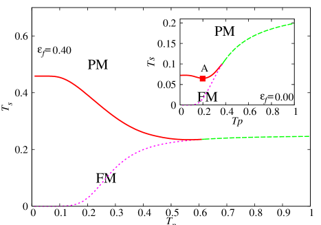
Figure 3: Phase diagram of the case-1 model on $T_{S}-T_{p}$ plane with $\alpha=0.45$ and $\epsilon_{f}=0.4$. The thick line represents the first-order phase transition. The symbols of lines are the same as those in Fig.1 The inset shows the phase diagram of the case-1 model with $\alpha=0.45$ and $\epsilon_{f}=0$.

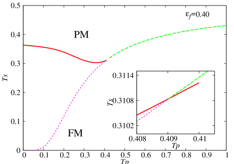
Figure 4: Phase diagram of the case-2 model with $\alpha=0.45$ and $\epsilon_{f}=0.40$. The symbols of lines are the same as those in Fig. 1. The inset shows an enlarged view near the multicritical point. The first-order-transition line intersects with the paramagnetic instability line.

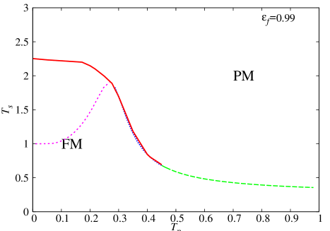
Figure 6: Phase diagram of the case-1 model $\alpha=0.45$ and $\epsilon_{f}=0.99$. The symbols of lines are the same as those in Fig. 1.

In this subsection, we discuss phase diagram with relatively large $\epsilon_{f}$. There is remarkable difference in the stability of ferromagnetic order between the case-1 and case-2 models. Fig. 5 shows a phase diagram of the case-1 model with $\epsilon_{f}=0.8$, in which the ferromagnetic phase exists stably up to extremely high temperature. As $\epsilon_{f}$ increases further, $T_{S}^{(1)}$ takes a finite value in the limit $T_{p}=0$ again, as shown in Fig. 6. Namely, in a finite range of $\epsilon_{f}$, $T_{S}^{(1)}$ diverges as a function of $T_{p}$ and then the ferromagnetic phase becomes stable even in the high $T_{S}$ limit. In contrast, the ferromagnetic phase boundary in the case-2 model changes modestly with $\epsilon_{f}$ increasing as shown in Fig. 4 and $T_{S}^{(1)}$ remains to be finite in the limit $T_{p}=0$ . This suggests that the difference of the time scales between the particle and the spin strongly affects on the stability of the ferromagnetic phase.

It would be helpful for making clear the issue mentioned above in the two models to see an instability condition of the paramagnetic phase. The paramagnetic instability line, $(T_{S}^{(pmi)},T_{p}^{(pmi)})$, on the $T_{S}-T_{p}$ plane is simply determined by the condition $\left.\frac{\partial^{2}\mathcal{F}}{\partial m^{2}}\right|_{m=0,\rho=\rho_{pm}}=0$, because off-diagonal term of a Hessian matrix of the free energy with respect to $m$ and $\rho$ vanishes in the paramagnetic phase. Then, the self-consistent equations for $\rho$, Eqs. (17) and (19), in the paramagnetic phase are simply reduced to the equation,

$$\rho_{0}^{(pm)} = \frac{e^{\beta_{p}(\epsilon_{f}\rho_{0}^{(pm)}-\alpha)}}{1+e^{\beta_{p}(\epsilon_{f}\rho_{0}^{(pm)}-\alpha)}},$$ (22)

where $\rho_{0}^{(pm)}$ denotes a solution of the equation in the paramagnetic phase. By using the solution of the equation, the instability condition for the case-1 model is given by

$$\beta_{S}J\left(1-\frac{J}{T_{p}}\rho_{0}^{(pm)}(1-\rho_{0}^{(pm)})-\frac{J}{T_{S}}{\rho_{0}^{(pm)}}^{2}\right)=0.$$ (23)

This yields the instability temperature $T_{S}^{(pmi)}$ as a function of $T_{p}$ expressed as

$$T_{S}^{(pmi)}(T_{p})=\frac{J{\rho_{0}^{(pm)}}^{2}}{1-(J/T_{p})\rho_{0}^{(pm)}(1-\rho_{0}^{(pm)})}.$$ (24)

When the denominator $1-(J/T_{p})\rho_{0}^{(pm)}(1-\rho_{0}^{(pm)})$ is zero, $T_{S}^{(pmi)}$ diverges and hence the ferromagnetic phase becomes stable even at $T_{S}=\infty$. As a trivial example, when $\epsilon_{f}=2\alpha$, $T_{S}^{(pmi)}$ goes to infinity at $T_{p}=1/4$. At $(\epsilon_{f},\alpha)=(0.90,0.45)$, the first-order-transition line and the paramagnetic instability line almost merge and the jump of thermodynamic quantities at first-order transition is quite weak in a wide region of $(T_{S},T_{p})$ plane. Because the instability line is located on the second-order transition or inside the ferromagnetic phase, the divergence of $T_{S}^{(pmi)}(T_{p})$ means the stability of ferromagnetic phase at an infinite $T_{S}$.

We show explicitly the stability of ferromagnetic phase in the case-1 model at $T_{p}=0$. In the case-1 model, the spins that are slow variable can fluctuate even at $T_{p}=0$. The particle configuration is adaptively determined for a given slow spin configuration by minimizing the free energy. For intermediate $\epsilon_{f}$, which is, to be precise, given by $\epsilon_{f}<1.45$ at $\alpha=0.45$, the paramagnetic state is an empty state at $T_{p}=0$, namely $m_{0}=0$ and $\rho_{pm}=0$. On the other hand, the self-consistent equations, Eq.(16) and Eq.(17), for the ferromagnetic solution, $m_{0}$ and $\rho_{0}^{(fm)}$, at $T_{p}=0$ are then

$$m_{0} = \pm\rho_{0}^{(fm)},$$ (25)

$$\rho_{0}^{(fm)} = \frac{e^{\beta_{S}\big{(}(J+\epsilon_{f})\rho_{0}^{(fm)}+\alpha\big{)}}}{e^{\beta_{S}\big{(}(J+\epsilon_{f})\rho_{0}^{(fm)}+\alpha\big{)}}+1}.$$ (26)

When $T_{S}$ increases to infinity, $\rho_{0}^{(fm)}$ decreases gradually down to $1/2$, but never reaches to zero. Consequently, the magnetization $m$ remains finite even at $T_{S}=\infty$. In fact, in the limit $T_{S}\rightarrow\infty$, the free-energy difference between the ferromagnetic and the paramagnetic solution takes the form $-\frac{J+\epsilon_{f}}{8}+\alpha/2$, that is the internal energy for the ferromagnetic solution. This yields the stability condition of the ferromagnetic phase as $\epsilon_{f}>4\alpha-J$. For example with $\alpha=0.45$ and $\epsilon_{f}=0.8$, as shown in Fig. 5, the ferromagnetic phase is extended up to very high $T_{S}$ temperature, although the instability line of the paramagnetic solution goes down to the origin.

For sufficiently large $\epsilon_{f}$, the paramagnetic solution is qualitatively changed by the effect of the attractive interaction. Then, $\rho_{0}^{(pm)}=1$ at $T_{S}\rightarrow\infty$ in the limit $T_{p}=0$ and the free-energy difference is modified to $-\frac{J+3\epsilon_{f}}{8}-\frac{\alpha}{2}$. The dense paramagnetic solution becomes dominant at $(T_{p},T_{S})=(0,\infty)$. Thus, the first-order transition temperature $T_{S}^{(1)}(T_{p})$ can diverges only in a finite range of $\epsilon_{f}$ in the case-1 model.

In the case-2 model, on the other hand, the spin variables fluctuate as fast degree of freedom for a given slow particle configuration. The paramagnetic instability condition is then given by

$$\beta_{p}J\left(1-\frac{1}{T_{S}}J\rho_{0}^{(pm)}\right)=0,$$ (27)

where $\rho_{0}^{(pm)}$ is again determined by Eq. (22). The $T_{p}$ dependent term coupled to ${\rho_{0}^{(pm)}}^{2}$ cancels out because of the symmetry of the fast spin variable. In the paramagnetic phase, the particle density $\rho_{0}^{(pm)}$ of the case-2 model is the same value as the case-1 model. Thus, $T_{S}^{(pmi)}$ could not diverge in any value of $\epsilon_{f}$ and $T_{p}$, in sharp contrast to the case-1 model. This is, however, an necessary condition but not the sufficient one for the finite transition temperature at $T_{p}=0$.

We see again the phase boundary at $T_{p}=0$. In the case-2 model, the only particle configuration that minimizes the partial free energy at $T_{p}=0$ contributes to the ensembles and the fast spin variables fluctuate under the resultant particle configurations. The self-consistent equation for $\rho_{0}^{(pm)}$ leads to $\rho_{0}^{(pm)}=0$ at $T_{p}=0$, while the corresponding equation for the ferromagnetic phase leads to a fully occupied solution with $\rho_{0}=1$. For the latter, the magnetization $m_{0}$ is determined by the equation

$$m_{0}=\tanh\beta_{S}Jm_{0},$$ (28)

under the condition $e^{\beta_{S}(\epsilon_{f}-\alpha)}\cosh\beta_{S}Jm_{0}>1$. Thus, $T_{S}^{(1)}$ never diverges and the ferromagnetic phase only emerges at most $T_{S}<1/J$. Actually, $T_{S}^{(1)}$ is obtained by solving the equation

$$0=\frac{1}{2}\big{(}Jm_{0}^{2}+\epsilon_{f}\big{)}-T_{S}\log\big{(}e^{\beta_{S}(\epsilon_{f}+\alpha)}\cosh\beta_{S}Jm_{0}\big{)},$$ (29)

which is derived from the condition that the free-energy difference becomes zero at the transition temperature.

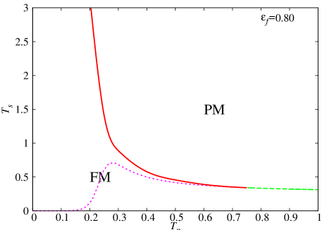
Figure 5: Phase diagram of the case-1 model with $\alpha=0.45$ and $\epsilon_{f}=0.80$. The symbols of lines are the same as those in Fig. 1.

V summary

We have studied phase transition of a non-equilibrium statistical-mechanical model that consists of two degrees of freedom with different time scales and heat baths, called two-temperature systems. A theoretical framework based on the replica method and its thermodynamical structure, which have been already given in the literatureCPS ; Dotsenko ; AP , are summarized. As a direct consequence of the structure, we have pointed out the existence of a Clausius-Clapeyron like relation in two-temperature systems, which enables us to link the topology of phase diagram and discontinuity of thermodynamic quantities at first-order transition. In particularly, a general condition to find the anomalous negative latent heat that is found in a specific spin modelAP is reduced to a simple topological constraint on the phase diagram. To be concrete, when the slope of the first-order phase boundary is a certain value determined by the retio of two temperatures, the negative latent heat appears. It should be worth noting that this criteria can be applied to any model including short-ranged models in finite dimensions.

We have also performed a mean-field analysis of two-temperature version of a spin-lattice gas model that has spins and particles as configurational variables. Generally, two-temperature systems are characterized by the Hamiltonian and time-scale order of two varibles. Even in the same Hamiltonian, phase diagram still depends on the choise of the time-scale order. We have studied phase diagram of the spin-lattice gas model for two different cases; one is that the spins are slow and the particles are fast, which is the same as that studied by APAP , and the other is alternative. Furthermore, the effect by introducing preferentially an attractive interaction for one of the two variables is studied. We have found that the general condition for the negative latent heat is satisfied in a parameter region both for two cases, suggesting that the negative latent heat is not accidental but frequently observed in two-temperature systems. By increasing the attractive interaction, the parameter region becomes narrow in common. On the other hand, qualitatively different properties are found in the phase diagram, such as the stability of the ferromagnetic order and the existence of the ferromagnetic-ferromagnetic transition. This indicates that the time-scale order plays a significant role in phase transitions and cooperative phenomena. An interesting and open problem would be to see if the results found in the spin-lattice gas model are preserved beyond the mean-field analysis, for instance in finite-dimensional short range models. In this direction, we further progress for the model up to the Bethe approximationNH2 .

- (1) M. C. Cross, and P. C. Hohenberg, Rev. Mod. Phys. 65, 851 (1993).
- (2) J. Marro,and R. Dickman, Non-equilibrium Phase Transitions in Lattice Models, (Cambridge University Press, Cambridge, 1999).
- (3) G. Odor, Rev. Mod. Phys. 76, 663 (2004).
- (4) P. D. Olmsted, and P. Goldbart Phys. Rev. A. 41, 4578 (1990)
- (5) B. Schmittman, and R. K. P. Zia, in Phase Transitions and Critical Phenomena, edited by C. Domb and J. L. Lebowitz (Academic Press, New York, 1995) Vol.17.
- (6) Z. Racz, in Slow relaxations and nonequilibrium dynamics in condensed matter, edited by J. -L. Barrat et al, (Springer-Verlag, 2002), cond-mat/0210435.
- (7) R. K. P. Zia, E. L. Plaestgaard, and O. G. Mouristen, Am. J. Phys. 70, 384 (2002).
- (8) A. E. Allahverdyan, and K. G. Petrosyan, Phys. Rev. Lett. 96, 065701 (2006).
- (9) R. W. Penney, A. C. C. Coolen, and D. Sherrington, J. Phys. A: Math. Gen. 26, 3681 (1993).
- (10) B. Wemmenhove, and N. S. Skantos, J. Phys. A: Math. Gen. 37, 7843 (2004).
- (11) S. I. Doronin, E. B. Feldman, E. I. Kuznetsova, G. B. Furman, S. D. Goren, Phys. Rev. B. 76, 144405 (2007).
- (12) M. Mezard, G. Parisi, and M. A. Virasoro, Spin-glass Theory and Beyond, (World Scientific, Singapore, 1987).
- (13) A. E. Allahverdyan, Th. M. Nieuwenhuizen, and D. B. Saakian, Eur. Phys. J. B. 16, 317 (2000).
- (14) V. Dotsenko, S. Franz and M. Mezard, J. Phys. 27, (1994) 2351.
- (15) R. O. Sokolovskii, Phys. Rev. B. 61, 36 (2000)
- (16) E. Fermi, Thermodynamics, (Dover, New York, 1956).
- (17) C. H. Nakajima and K. Hukushima, in preparation.