From Capillary Condensation to Interface Localization Transitions in Colloid Polymer Mixtures Confined in Thin Film Geometry

Abstract

Monte Carlo simulations of the Asakura-Oosawa (AO) model for colloid-polymer mixtures confined between two parallel repulsive structureless walls are presented and analyzed in the light of current theories on capillary condensation and interface localization transitions. Choosing a polymer to colloid size ratio of $q=0.8$ and studying ultrathin films in the range of $D=3$ to $D=10$ colloid diameters thickness, grand canonical Monte Carlo methods are used; phase transitions are analyzed via finite size scaling, as in previous work on bulk systems and under confinement between identical types of walls. Unlike the latter work, inequivalent walls are used here: while the left wall has a hard-core repulsion for both polymers and colloids, at the right wall an additional square-well repulsion of variable strength acting only on the colloids is present. We study how the phase separation into colloid-rich and colloid-poor phases occurring already in the bulk is modified by such a confinement. When the asymmetry of the wall-colloid interaction increases, the character of the transition smoothly changes from capillary condensation-type to interface localization-type. The critical behavior of these transitions is discussed, as well as the colloid and polymer density profiles across the film in the various phases, and the correlation of interfacial fluctuations in the direction parallel to the confining walls. The experimental observability of these phenomena also is briefly discussed.

I INTRODUCTION AND OVERVIEW

When fluid systems are confined in nanoscopic pores or channels, one expects that the phase behavior can be profoundly modified 1 ; 2 ; 3 ; 4 ; 5 ; 6 ; 7 ; 8 ; 9 ; 10 . Such effects have found an increasing attention recently, for instance because of the current interest to fabricate devices of nanoscopic size and to manipulate chemical reactions in nanoscopic reaction volumes (“lab on a chip”), etc. 11 ; 12 ; 13 ; 14 ; 15 ; 16 . In addition, porous materials with pores of nanoscopic widths are useful as catalysts or for applications such as mixture separation, pollution control, etc. 6 ; 17 ; 18 ; 19 .

However, such applications often are based on empirical knowledge, the theoretical understanding of confined fluids still being rather limited 6 ; 7 ; 8 ; 9 ; 10 . In order to make progress with the theoretical description of fluids under confinement by the methods of statistical thermodynamics, it is desirable to start with relatively simple model systems, where both the geometry of confinement is well characterized, and the relevant interactions among the fluid particles and between the fluid particles and the confining solid surfaces are sufficiently well understood. Last but not least, suitable experimental tools should be in principle available to put the theoretical predictions to a test.

For these purposes it is hence useful to consider colloidal suspensions 20 ; 21 ; 22 ; 23 ; 24 , exploiting the analogy between colloidal fluids and fluids formed from small molecules, but taking advantage of the much larger length scales (in the $\mu$m range), of the colloidal particles. Such systems allow detailed experiments in which individual particles can be tracked through space in real time using confocal microscopy techniques 25 . Particularly useful systems in the present context are colloid-polymer mixtures, which can undergo in the bulk a liquid-vapor like phase separation into a colloid-rich phase (the “liquid”) and a colloid-poor phase (the “vapor”) 23 ; 26 . This phase separation is due to the (entropic) depletion attraction between the colloids caused by the polymers. A very simple model, due to Asakura and Oosawa 27 and Vrij 28   describes the resulting phase separation in the bulk 29 ; 30 ; 31 ; 32 ; 33 in excellent qualitative agreement with the experiment 23 . While initially it was thought that mean field theory 29 accounts very accurately for the Monte Carlo (MC) simulation results 30 ; 31 of this Asakura-Oosawa (AO) model, a more extensive MC simulation study 32 ; 33 revealed clear evidence for Ising-like critical behavior 34 over a broad regime of control parameters.

When such a colloid-polymer mixture is confined by hard walls, also a depletion attraction of the colloids and the walls occurs 35 and can cause (in semi-infinite geometry 36 ; 37 ; 38 ; 39 ; 40 ) the formation of wetting layers 41 ; 42 ; 43 ; 44 ; 45 ; 46 . Due to the very low interfacial tension between unmixed phases 47 ; 48 ; 49 ; 50 , thermally activated capillary-wave fluctuations 51 ; 52 ; 53 ; 54 ; 55 are readily observable in experiment 56 and simulation 50 . The phase behavior of colloid-polymer mixtures in confinement can be also studied experimentally. Therefore, this issue has been addressed in recent computer simulation studies, considering the confinement of colloid-polymer mixtures by two parallel hard walls a distance $D$ apart 9 ; 57 ; 58 ; 59 . These studies have confirmed the fact that lateral phase separation in a thin film geometry exhibits a critical behavior belonging to the class of the two-dimensional Ising model 58 . Also the the scaling relations of Fisher and Nakanishi 60 have been verified. Unlike the case of confinement of small molecule fluids in nanopores, the size of the particles in colloidal fluids by far exceeds the scale of the atomistic corrugation of the pore walls, and hence the effects of this corrugation on the packing of particles near the walls 61 ; 62 need not be considered here.

A very useful aspect of colloidal suspensions is that interactions among such particles can be tuned by suitable surface treatment 20 ; 21 ; 22 ; 63 . E.g., a short-range repulsion between colloidal particles often is created by coating them with a polymer brush 63 ; 64 . Similarly, one could cancel (partially or completely) the depletion attraction of colloids towards a hard wall by coating the latter with a polymer brush, choosing the grafting density and chain length of these flexible polymers appropriately. In a colloid-polymer mixture, however, for moderate chain stretching in the polymer brush the polymers in the solution still can penetrate into the brush, experiencing hence a much weaker interaction than the colloidal particles. Only for strongly stretched chains, as occurring in very dense polymer brushes 65 , a repulsion of the polymer coils in the solution would result as well, even if the chemical nature of the polymers in the solution and in the brush is identical (“autophobicity effect” 66 ; 67 ).

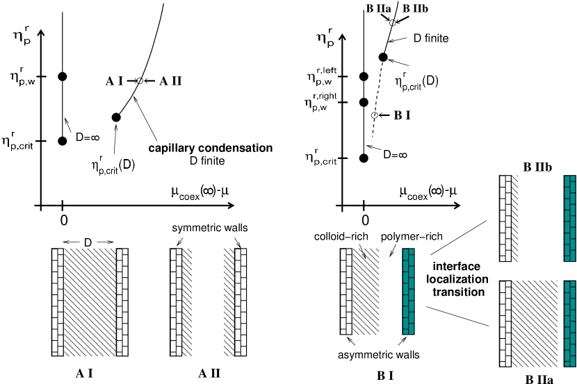
Figure 1: Schematic phase diagrams of a colloid-polymer mixture confined between two parallel walls a distance $D$ apart, in the grand-canonical ensemble where the polymer reservoir packing fraction $\eta_{\rm p}^{\rm r}$ is used as ordinate axis and the difference between the chemical potential of the colloids at bulk phase coexistence $\mu_{\textrm{coex}}(D=\infty)$ and the actual chemical potential of the colloids is used as abscissa (upper part). Phase coexistence in the bulk occurs along the vertical straight lines at $\mu_{\textrm{coex}}(\infty)-\mu=0$. The left phase diagram refers to the case of symmetric walls, the right one to asymmetric walls. The lower part of the figure indicates the phases that occur in these phase diagrams (shaded regions denote colloid-rich domains): In the case of symmetric walls, a colloid-rich phase (AI) coexists along the line $\mu=\mu_{\textrm{coex}}(D,\eta_{\rm p}^{\rm r})$ with a colloid-poor phase (AII). In the case of asymmetric walls, the analogous phases are BIIa, BIIb; BIIa differs from $A_{I}$ by the presence of a layer at the right walls where polymers are enriched, and BIIb differs from AII by the fact that a surface enrichment layer of colloids exists only at the left wall. Finally, a state with a delocalized interface between colloid-rich and polymer-rich phases (BI) exists along the continuation of the line $\mu=\mu_{\textrm{coex}}(D,\eta_{\rm p}^{\rm r})$ beyond the critical point $(\eta_{\rm p,crit}^{\rm r}(D))$, dotted line. The transition from BI to either BIIa or BIIa when one moves along the dotted line is termed interface localization transition. For further explanations cf. text.

This tunability of the wall-colloid interactions opens the possibility to realize a situation of a slit pore with asymmetric walls: suppose the left wall is simply a hard wall, attractive for the colloids, and the right wall a coated hard wall, repulsive for the colloids (Fig. 1) 68 . With a colloid-polymer mixture confined between such asymmetric walls, the possibility arises to realize the “interface localization transition” 7 ; 9 ; 69 ; 70 ; 71 ; 72 ; 73 ; 74 ; 75 ; 76 ; 77 ; 78 . This transition is illustrated in Fig. 1. Here, the so-called “polymer reservoir packing fraction” is defined by $\eta^{\rm r}_{\rm p}\equiv(4\pi/3)R_{\rm p}^{3}\exp(\mu_{\rm p}/k_{B}T)$ (with $R_{\rm p}$ and $\mu_{\rm p}$ the radius and the chemical potential of the polymers, respectively) and plays the role of inverse temperature when we compare the behavior to that of a fluid of small molecules that undergoes a liquid-vapor transition. While in the bulk colloid-polymer mixture phase separation sets in when the variable $\eta_{\rm p}^{\rm r}$ exceeds the critical value $\eta_{\rm p,crit}^{\rm r}$, this transition is rounded in the thin film. Starting out from a layer enriched with colloids on the left wall and enriched with polymers at the right wall, a stratified domain structure forms, with a domain wall separating the colloid-rich phase in the left part and the polymer-rich phase in the right part of the slit pore (state BI in Fig. 1). Only at a much larger value $\eta_{\rm p,crit}^{\rm r}(D)$ a sharp phase transition occurs in the thin film, with the colloid-polymer interface being bound either to the right wall (phase B IIa) or to the left wall (phase B IIb). Along the line $\mu=\mu_{\rm coex}(D,\eta_{\rm p}^{\rm r})$ these two phases may coexist.

Of course, in an experiment one does not have at one’s disposal the intensive variables $\mu$ and the “polymer reservoir packing fraction” $\eta_{\rm p}^{\rm r}$, but rather the volume fractions of colloids and polymers,

$$\eta_{\rm c}=\frac{4\pi}{3}R^{3}_{\rm c}N_{\rm c}/V\;,\quad\eta_{\rm p}=\frac{4\pi}{3}R_{\rm p}^{3}N_{\rm p}/V\;,$$ (1)

where $V$ is the volume of the system, $R_{\rm c}$ the radius of the spherical colloidal particles, and $N_{\rm c}$, $N_{\rm p}$ are the particle numbers of colloids and polymers, respectively. Since $\eta_{\rm c}$, $\eta_{\rm p}$ are densities of extensive thermodynamic variables, the first order transition lines $\mu_{\textrm{coex}}(D,\eta_{\rm p}^{\rm r})$ in the plane of variables $\eta_{\rm c}$, $\eta_{\rm p}$ are split into two phase coexistence regions. Bringing the thin film from the one-phase region to inside the two-phase region (e.g. by adding polymers to the solution), one creates a state of the slit pore where in parts of the system the interface is bound to the left wall and in other parts it is bound to the right wall. These phases are then separated by interfaces running across the film from the left to the right wall (or vice versa). A similar phase coexistence between the two phases AI, AII occurs in the case of capillary condensation-like transitions for symmetric walls (left part of Fig. 1). As always, the amounts of the coexisting phases is controlled by the lever rule.

In the limit $D\rightarrow\infty$ of the film thickness, we recover a semi-infinite system and then wetting transitions are expected to occur, so that, in the symmetric wall case, in the region $\eta^{\rm r}_{\rm p,crit}<\eta_{\rm p}^{\rm r}<\eta_{\rm p,w}^{\rm r}$ for $\mu=\mu_{\textrm{coex}}(\infty)$ both walls are (completely) wet, while for $\eta_{\rm p}^{\rm r}>\eta_{\rm p,w}^{\rm r}$ the walls are nonwet (“incomplete wetting” 36 ; 37 ; 38 ; 39 ; 40 ). In fact, the colloid-rich surface enrichment layers indicated for the phase AII are the precursors of wetting layers that appear when $D\rightarrow\infty$. Of course, no (infinitely thick 36 ; 37 ; 38 ; 39 ; 40 ) true wetting layer fits into a thin film of finite thickness $D$, and thus the wetting transition at $\eta_{\rm p}^{\rm r}=\eta_{\rm p,w}^{\rm r}$ (which we have assumed to be of second order 36 ; 37 ; 38 ; 39 ; 40 ) is rounded off in the thin film.

For asymmetric walls in the limit $D\rightarrow\infty$ the wetting transitions at both walls will occur, in general, for different values of $\eta_{\rm p}^{\rm r}$ at both walls. In Fig. 1 we have arbitrarily assumed that $\eta_{\rm p,w}^{\rm r,left}>\eta_{\rm p,w}^{\rm r,right}$. In the simplistic Ising model with “competing surface magnetic fields” 69 ; 70 ; 71 ; 72 ; 73 ; 74 $H_{1}$ and $H_{D}$, one can consider a situation with $H_{D}=-H_{1}$, where these transitions then coincide, $\eta_{\rm p,w}^{\rm r,left}=\eta_{\rm p,w}^{\rm r,right}$. However, such a special symmetry never is expected for a colloid-polymer mixture (which has an asymmetric phase diagram already in the bulk). Note, however, that for $D\rightarrow\infty$ one does not expect that for interface localization transitions $\eta_{\rm p,crit}^{\rm r}(D)$ converges to the bulk critical point, $\eta_{\rm p,crit}^{\rm r}$: rather one expects a convergence towards the wetting transition which is closest to the bulk transition 7 .

In the present paper, we shall present evidence from Monte Carlo simulations that the scenario sketched in Fig. 1 is correct, and we shall characterize the behavior of colloid-polymer mixtures confined by asymmetric walls in detail, considerably extending preliminary work 68 . Extensive results for the case of symmetric walls have been presented earlier 58 ; 59 . As in previous studies in the bulk 32 ; 33 the simulations are carried out mostly in the grand-canonical ensemble, using a dedicated grand-canonical cluster algorithm 32 together with re-weighting schemes such as successive umbrella sampling 79 . Phase transitions are analyzed by finite size scaling methods 80 ; 81 ; 82 , varying suitably the lateral linear dimensions $L$ along the walls. For a description of these techniques, the reader should consult our earlier work 58 ; 59 .

In Sec. II we now present a study of the “soft mode” phase 72 BI for a relatively thick film (thickness $D=10$ colloid diameters). Such phases with delocalized interfaces are of great interest due to their large interfacial fluctuations 72 ; 73 ; 74 ; 83 ; 84 , and consequences of such fluctuations have been seen in experiments both on polymer blends 85 and colloid-polymer mixtures 46 . Sec. III then gives a discussion of the interface localization transition for an ultrathin film ($D=3$), attempting to verify the above statement that the critical exponents should be those of the two-dimensional Ising model. Sec. IV discusses the phase behavior when both film thickness and the strength of the short range colloid-wall repulsion are varied. Finally, Sec. V summarizes some conclusions.

II FORMATION AND PROPERTIES OF THE INTERFACE IN THE SOFT MODE PHASE

All our Monte Carlo simulations refer to the standard Asakura-Oosawa (AO) model and use the same size ratio $q=R_{\rm p}/R_{\rm c}=0.8$ as the previous work in the bulk 32 ; 33 and for symmetric walls 58 ; 59 . In this case, it is known that the critical point in the bulk occurs at 32 ; 33

$$\eta_{\rm p,crit}^{r}=0.766\pm 0.002,\quad\eta_{\rm c,crit}=0.1340\pm 0.0002,\quad\eta_{\rm p,crit}=0.3562\pm 0.0006,$$ (2)

and also the coexistence curve between the colloid-rich phase ($\eta_{{\rm c},\ell}$) and the polymer-rich phase $(\eta_{{\rm c},v})$ is known rather precisely, as well as the interfacial tension 32 ; 33 ; 50 . We now consider a $L\times L\times D$ geometry, where all lengths are measured in units of the colloid diameter $2R_{\rm c}$, and periodic boundary conditions are applied in $x$ and $y$-directions only. For the thickness $D$, the values $D=3$, 5, 7, and 10 are used, while the linear dimension $L$ in parallel direction is chosen in the range from $L=15$ to $L=30$. The left wall, located at $z=0$, is taken purely repulsive for both colloids and polymers. As for the interaction between the colloidal particles (which is infinite if two colloids overlap and zero else, as well as the colloid-polymer interaction which also is infinite if a colloid particle overlaps a polymer and zero else), we take a hard wall repulsion,

$$U_{\rm w,c}^{\ell}(z)=\infty,\;z<R_{\rm c}, U_{\rm w,c}^{\ell}(z)=0,\;z>R_{\rm c},$$ (3)

$$U_{\rm w,p}^{\ell}(z)=\infty,\;z<R_{\rm p}, U_{\rm w,p}^{\ell}(z)=0,\;z>R_{\rm p},$$ (4)

for both colloids $[U_{\rm w,c}^{\ell}(z)]$ and polymers $[U_{\rm w,p}^{\ell}(z)]$. At the right wall, however, we add a square well potential of strength $\varepsilon$ and with an additional range $R_{\rm c}$. Thus, the potential acting on the colloids is

$$U_{\rm w,c}^{\rm r}(z)=0, z<D-2R_{\rm c},$$ (5a)

$$U_{\rm w,c}^{\rm r}(z)=\varepsilon, D-2R_{\rm c}<z<D-R_{\rm c},$$ (5b)

$$U_{\rm w,c}^{\rm r}(z)=\infty, z>D-R_{\rm c}.$$ (5c)

This square well potential [Eq. (5b)] could be realized by a polymer brush of low grafting density and height $R_{\rm c}$, for instance, so that the region of $z$ where the colloid penetrates into the brush leads to a finite energy penalty $\varepsilon$ only (note that we use the convention that the temperature $k_{B}T=1$; of course, one could also consider square well potentials of arbitrary range). For the polymers, on the other hand, the interaction is taken to be of the same type as in Eq. (4),

$$U_{\rm w,p}^{\rm r}(z)=0,\;z<D-R_{\rm p},\quad U_{\rm w,p}^{\rm r}(z)=\infty,\;z>D-R_{\rm p}.$$ (6)

This potential models the interactions of polymers with a hard wall coated with polymer brushes: Under good solvent or Theta solvent conditions 86 , polymers can overlap with weakly stretched polymer brushes with little free energy cost.

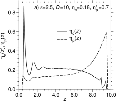
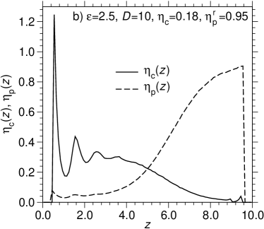
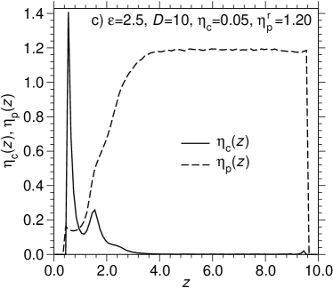
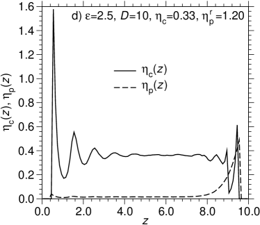
Figure 2: Colloid concentration profiles $\eta_{\rm c}(z)$ and polymer concentration profiles $\eta_{\rm p}(z)$ as a function of $z$ for a thin film with asymmetric walls. At $z=0$ there is a hard wall, where the potentials $U_{\rm w,c}^{\ell}(z)$ and $U^{\ell}_{\rm w,p}(z)$ [Eqs. (2), (3)] act on colloids (c) and polymers (p). At $z=D$ there is another hard wall for both types of particles, with an additional square well repulsion acting on the colloids only [Eqs. (3), (4), (5a), (5b), (5c)] with a strength $\varepsilon=2.5$. Profiles were obtained at $\eta_{\rm c}=0.18$, $\eta_{\rm p}^{\rm r}=0.70$ (a), $\eta_{\rm c}=0.18$, $\eta_{\rm p}^{\rm r}=0.95$ (b), $\eta_{\rm c}=0.05$, $\eta_{\rm p}^{\rm r}=1.20$ (c), and $\eta_{\rm c}=0.33$, $\eta_{\rm p}^{\rm r}=1.20$ (d). For profiles (c) and (d), the choices $\eta_{\rm c}=0.05$ and 0.33 roughly correspond to the two branches of the coexistence curve in the bulk.

It turns out that a phase behavior as sketched in the right part of Fig. 1 occurs if $\varepsilon\geq 2.5$. Figure 2 presents some typical profiles of the average local volume fraction of colloids $\eta_{\rm c}(z)$ and polymers $\eta_{\rm p}(z)$ across the slit pore, for the case $\varepsilon=2.5$ and $D=10$. Panel (a) shows the profiles for $\eta_{\rm c}=0.18$ and $\eta_{\rm p}^{\rm r}=0.7$, corresponding to a state point where the bulk colloid-polymer mixture is still in the one-phase region. Nevertheless, the profiles of $\eta_{\rm c}(z)$ and $\eta_{\rm p}(z)$ exhibit pronounced inhomogeneities: the polymer profile $\eta_{\rm c}(z)$ displays a pronounced peak close to the right wall, and decays with increasing distance from the right wall to a plateau, almost independent of $z$, in the regime $3\leq z\leq 6$. Very close to the left wall, where the volume fraction of colloids is strongly enhanced, the concentration of polymers is also inhomogeneous (indirectly induced by the colloids, since polymers and colloids must not overlap), before $\eta_{\rm p}(z)$ abruptly decreases to zero for $z=R_{\rm p}$. The colloid profile $\eta_{\rm c}(z)$ shows a very pronounced peak close to $z=R_{\rm c}$, on the other hand, which can be attributed to the depletion attraction of the colloids to the hard wall. One can recognize a second peak near $z=1.6$ and a weak third peak near $z=2.5$, these peaks represent the well-known “layering” of hard particles near smooth repulsive walls. In the central part of the thin film, for $3\leq z\leq 6$, the profile $\eta_{\rm c}(z)$ is almost flat; thus the surface enrichment of the colloidal particles at the hard wall is a short range effect. In the regime near the right walls, where the polymers are attracted, we recognize first a smooth decrease of $\eta_{\rm c}(z)$ in the range where the pronounced increase of $\eta_{\rm p}(z)$ sets in. For $z=D-2R_{\rm c}=9$, where the additional repulsive potential sets in, a downward step in $\eta_{\rm c}(z)$ occurs, as expected.

It is interesting to contrast the behavior in panel (a), showing surface enrichment of colloids (left) and polymers (right) at the walls confining an otherwise homogeneous mixture, with the behavior in panel (b), which refers to a state where in the bulk phase separation has occurred. Indeed, Fig. 2b gives rather clear evidence for a phase separation in the $z$-direction perpendicular to the confining walls, of the type denoted as BI in Fig. 1. The polymer rich phase occurs on the right side of the thin film, and $\eta_{\rm p}(z)$ reaches very small values for $z\leq 4$. Near $z=6$ we recognize inflection points in both profiles $\eta_{\rm p}(z)$, $\eta_{\rm c}(z)$ as are typical for interfaces between coexisting phases. Again the profile $\eta_{\rm c}(z)$ exhibits the typical layering oscillations for small $z$. No such layering occurs for the polymers near $z=D$, of course, since the polymer-polymer interaction is zero, the polymer-rich phase is like a dense ideal gas.

Panels 2c and 2d illustrate states corresponding to the phases BIIb and BIIa in Fig. 1, respectively. In the polymer-rich phase the interface position is at about $z=2.5$, and unlike Fig. 2a (where the interface is freely fluctuating in the center of the slit pore) the width of the interface is only about two colloid diameters. Such a state is typical for a colloid-polymer interface tightly bound to the left wall. Figure 2d is the counterpart showing the profiles in the colloid-rich phase, where almost all polymers are expelled, apart from the immediate neighborhood of the right wall.

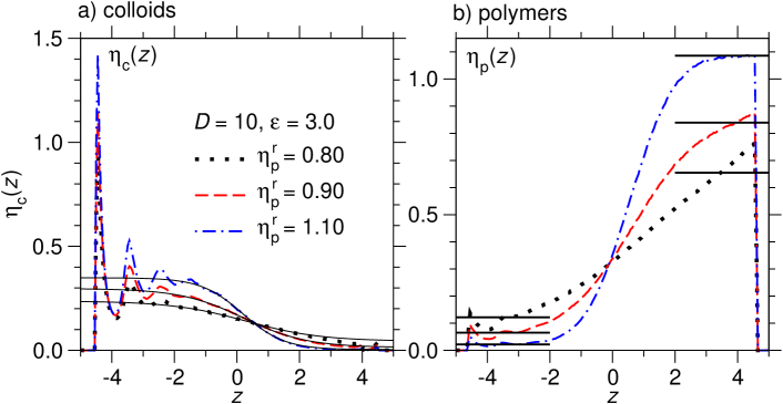
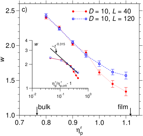
Figure 3: Colloid density profiles $\eta_{\rm c}(z)$ (a) and polymer density profiles $\eta_{\rm p}(z)$ (b) plotted vs. $z$ for the case $\varepsilon=3.0$, $D=10$, and choosing the average value of $\eta_{\rm c}$ equal to the diameter $\delta$, $\delta=(\eta_{\rm c}^{v}+\eta_{\rm c}^{\ell})/2$. Here the origin at $z=0$ is put into the center of the slit pore. Broken curves denote fits with tanh profiles, as described in the text. Part (c) shows the dependence of the width $w$ on $\eta_{\rm p}^{\rm r}$. Critical values $\eta_{\rm p,crit}^{\rm r}$ in the bulk and in the thin film $\eta_{\rm p,crit}^{\rm r}(D)$ are shown by arrows. Squares are for the choice $D=10$, $L=120$, circles for $D=10$, $L=40$. The insert shows a log-log plot of $w$ vs. $\eta_{\rm p}^{\rm r}/\eta_{\rm p,crit}^{\rm r}-1$. The solid line in the insert is a fit with a power law with the exponent $\nu/2=0.315$ (see text).

We conclude that these profiles do give qualitative evidence for the existence of all three phases BI, BIIa and BIIb in Fig. 1. We now study the phase with the delocalized interface (BI) more closely. In particular, we are interested in how the interfacial profiles change when the inverse-temperature-like variable $\eta_{\rm p}^{\rm r}$ is varied (Fig. 3). Defining an order parameter $m$ and the coexistence diameter $\delta$ as follows,

$$m=(\eta_{\rm c}^{\ell}-\eta_{\rm c}^{v})/2,\quad\delta=(\eta_{\rm c}^{v}+\eta_{\rm c}^{\ell})/2,$$ (7)

we choose the average volume fraction of the colloids such that $\eta_{\rm c}=\delta$, and we attempt to fit the colloid density profile by a tanh function,

$$\eta_{\rm c}(z)=\delta-m\tanh[(z-z_{0})/w]\quad;$$ (8)

here $z_{0}$ is the position of the interface center and $w$ is the interfacial width. Fig. 3a shows that Eq. (8) provides a good fit of the colloid density profile, for all values of $\eta_{\rm p}^{\rm r}$ from 0.90 to 1.10. For $\eta_{\rm p}^{\rm r}=0.80$, however, the profile is extremely wide, due to the proximity of the critical point in the bulk [Eq. (1)], and then the fit is less convincing. Indeed, the polymer density profile $\eta_{\rm p}(z)$, Fig. 3b, for $\eta_{\rm p}^{\rm r}=0.8$ does not even exhibit an inflection point, while for all larger values of $\eta_{\rm p}^{\rm r}$ an inflection point clearly is present (it occurs roughly at $z=z_{0}$, the inflection point of the polymer density profile, which is roughly at $z_{0}\approx 0.20\pm 0.05$).

Of course, one notes that $\eta_{\rm c}(z)$ does not reach the regime of homogeneous “liquid” density $\eta_{\rm c}^{\ell}$, since for $z\leq-1.5$ in Fig. 3a the layering effect caused by the repulsive wall at $z=-5$ already sets in. Likewise, the surface enrichment of the polymers at the right wall distorts the profiles for $z\geq 3.5$ in Fig. 3b. We also note that the profiles seem to have common intersection points (which do not coincide with $z_{0}$, since both $m$ and $\delta$ depend on $\eta_{\rm p}^{\rm r}$). The common intersection point of the colloid profiles is at $z=0.5\pm 0.05$, while the common intersection point of the polymer profile is at $z=0.0\pm 0.1$. Presumably, these common intersection points are just numerical coincidences, and will not occur in the general case (using other choices of $\varepsilon$ and $D$, for instance). However, the statistical effort for the data in Fig. 3 is rather substantial, and hence no such systematic parameter variation has been attempted.

Figure 3c shows that the effective interfacial width $w$ extracted from the fit to Eq. (8) increases from about $w\approx 1.5$ near the critical point of the thin film (the estimation of thin film critical points is discussed in the following sections) to about $w\approx 2.4$ for $\eta_{\rm p}^{\rm r}=0.8$. However, it is important to recall that the width $w$ of the interface in the “soft mode” phase depends on both $\eta_{\rm p}^{\rm r}$ and the total film thickness $D$ 83 ; 84 ; 85 ; 87 . This complicated behavior results because the “intrinsic interfacial profile” 88 ; 89 is broadened by capillary waves 51 ; 52 ; 53 ; 54 ; 55 , but the long-wavelength part of the capillary wave spectrum is suppressed by the effective interface potential 38 ; 39 caused by the walls. For short range forces due to the walls, as occurring here, the corresponding prediction for the mean square width is 83 ; 84 ; 85 ; 87

$$w^{2}=w_{0}^{2}[1+\frac{\omega\pi/4}{2+\omega}\frac{D}{w_{0}}]+\;\textrm{const}$$ (9)

Here, $w_{0}$ is the “intrinsic width”, which should be related to the correlation length $\xi_{\rm b}$ along the coexistence curve in the critical region, $w_{0}=2\xi_{\rm b}$, while the wetting parameter $\omega$ 38 ; 39 ; 40 ; 90 ; 91 ; 92 ; 93 for Ising-like systems is $\omega\approx 0.8$ and the (unknown) constant due to the short wavelength cutoff needed in the capillary wave spectrum 83 ; 84 ; 85 can be neglected near the critical point of the bulk. The intrinsic width should then vary with $\eta_{\rm p}^{\rm r}$ as

$$w_{0}=\hat{w}_{0}(\eta_{\rm p}^{\rm r}/\eta_{\rm p,crit}^{\rm r}-1)^{-\nu},\quad\quad\nu\approx 0.63,$$ (10)

with an amplitude factor $\hat{w}_{0}$ which is presumably in the range $0.2\leq\hat{w}_{0}\leq 0.5$ (it is not accurately known since an unambiguous separation of intrinsic width and capillary wave broadening is hardly possible in interfacial profiles 50 ; 87 ). Since for the chosen values of $\eta_{\rm p}^{\rm r}$ we have $D\gg w_{0}$ for $D=10$ and $(\omega\pi/4)/(2+\omega)\approx 0.224$, we expect that $w\approx 1.497\sqrt{w_{0}}$ in our case, i.e. $w$ in Fig. 3c should increase with an exponent $\nu/2$. Disregarding the results for $\eta_{\rm p}^{\rm r}=0.8$ and $\eta_{\rm p}^{\rm r}=0.85$, which are too close to $\eta_{\rm p,crit}^{\rm r}$ and hence unreliable due to finite size effects, we find that the remaining data for $L=120$ can be nicely fitted to a critical power law with the expected exponent $\nu/2=0.315$ (see insert of Fig. 3c).

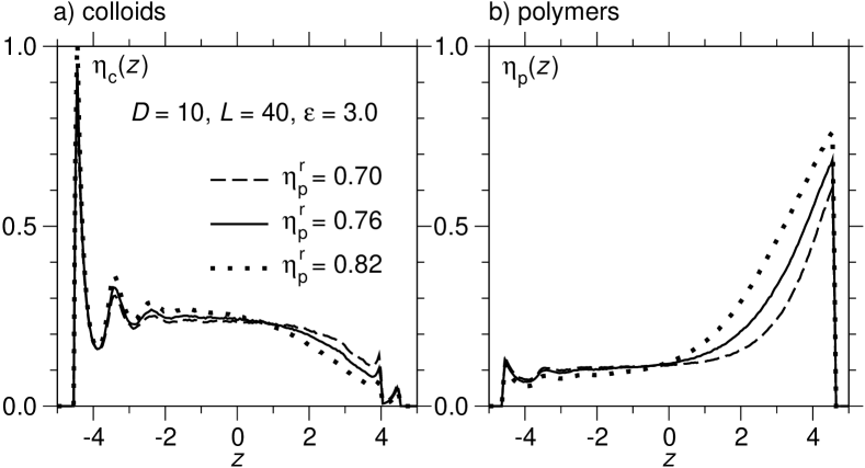
Figure 4: Density profiles $\eta_{\rm c}(z)$ (left part) and $\eta_{\rm p}(z)$ (right part) for the case $D=10$, $L=40$, $\varepsilon=3$ and $\eta_{\rm c}=0.195$. Three choices of $\eta_{\rm p}^{\rm r}$ are included, as indicated.

Thus, it clearly would be of interest to obtain reliable data close to the bulk critical point, but then much larger systems would be required, and this would require very substantial computer resources, that are not available to us. But we emphasize the fact that no singular behavior can be observed when at fixed $D$ we vary $\eta_{\rm p}^{\rm r}$ throughout the bulk critical region, passing the critical point. As an example, Fig. 4 shows density profiles for the case $D=10$, $\eta_{\rm c}=0.195,L=40$ and three values of $\eta_{\rm p}^{\rm r}$ close to $\eta_{\rm p,crit}^{\rm r}$ [Eq. (1)]. One sees that profiles for $\eta_{\rm p}^{\rm r}$ slightly above $\eta_{\rm p,crit}^{\rm r}$ and slightly below it are hardly distinct from each other, all changes with respect to $\eta_{\rm p}^{\rm r}$ are very gradual.

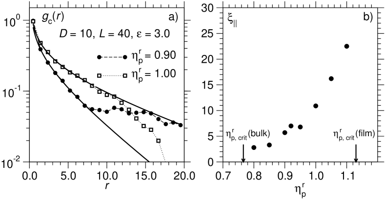
Figure 5: (a) Radial distribution function $g_{\rm c}(r)$ of the colloidal particles, considering only distances $r$ parallel to the walls, and particles confined in the interfacial region $z_{0}-w<z<z_{0}+w$, for the case $D=10$, $L=40$, $\eta_{\rm c}=0.195$, $\varepsilon=3$ and two choices of $\eta_{\rm p}^{\rm r}$, as indicated. Curves are fits to Eq. (11). (b) Plot of the parallel correlation length $\xi_{||}$ extracted from fits as shown in part (a), versus $\eta_{\rm p}^{\rm r}$.

A very interesting property is the correlation function of the colloidal particles in the interfacial region, $z_{0}-w<z<z_{0}+w$ (see Fig. 5). If we were to consider an unconfined interface, the capillary wave fluctuations would cause a power law decay of these fluctuations. Due to the confinement, the interface feels an effective potential, and this leads to the existence of a finite correlation length $\xi_{||}$ of interfacial fluctuations, as discussed extensively in the literature 72 ; 74 ; 83 ; 84 ; 85 ; 87 . In simulations of a model for a symmetrical polymer mixture confined between competing walls, this correlation length was studied as a function of film thickness. Here we rather study this quantity as the interface localization transition is approached. Figure 5a shows that the radial distribution function of colloidal particles in the interfacial regions is well described by the formula

$$g_{\rm c}(r)=\textrm{const}\,\exp(-r/\xi_{||})/\sqrt{r}\quad.$$ (11)

Equation (11) was also shown to work very well in the case of the symmetric polymer mixture 83 . When $\eta_{\rm p}^{\rm r}$ approaches the value $\eta_{\rm p,crit}^{\rm r}(D)$, one sees a strong increase of $\xi_{||}$, reflecting the expected critical divergence of $\xi_{||}$ at the interface localization transition [which occurs at about $\eta_{\rm p,crit}^{\rm r}(D)\approx 1.13\pm 0.03$]. Arguments have been given to show that for large enough $D$ there is a region of mean-field like behavior, where $\xi_{||}\propto(1-\eta_{\rm p}^{\rm r}/\eta_{\rm p,crit}^{\rm r}(D))^{-\nu_{||}}$ with $\nu_{||}=1/2$, while very close to $\eta_{\rm p,crit}^{\rm r}(D)$ the critical behavior should fall in the class of the two-dimensional Ising model 74 , $\nu_{||}=1$. However, the accuracy of the data in Fig. 5b does not warrant an analysis of this crossover behavior.

III INTERFACE LOCALIZATION TRANSITION IN VERY THIN FILMS

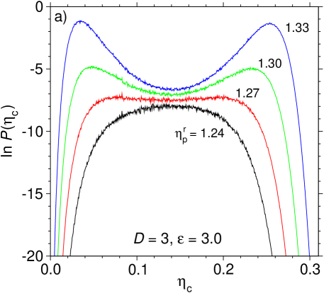
Figure 6: (a) Logarithm $\ln P(\eta_{\rm c})$ plotted vs. $\eta_{\rm c}$ for the case $D=3$, $L=15$, $\varepsilon=3.0$, and four values of $\eta_{\rm p}^{\rm r}$. (b) $U_{4}$ plotted vs. $\eta_{\rm p}^{\rm r}$, for the case $D=3$, $\varepsilon=3.0$, and various choices of $L$, as indicated. The horizontal broken line indicates the range where intersections occur, $1.295\leq\eta_{\rm p,crit}^{\rm r}(D)\leq 1.305$. The insert shows a log-log plot of $Y_{1}=dU_{4}/d\eta_{\rm p}^{\rm r}$ versus $L$. Broken straight line in the insert illustrates a slope $1/\nu_{||}=1.035$.

Following the procedures used in our earlier study of capillary condensation in the AO model, we carried out a finite size scaling analysis of the model with $\varepsilon=3.0$ for a slit pore which is only $D=3$ colloid diameters thick. Varying the chemical potential and applying successive umbrella sampling 79 , the probability distribution $P(\eta_{\rm c})$ is recorded. Applying suitable re-weighting techniques 94 , one can apply the equal area rule 95 ; 96 to determine the chemical potential $\mu_{\textrm{coex}}$ where the peak of $P(\eta_{\rm c})$ representing the vapor-like phase and the peak representing the liquid-like phase have equal weight. Figure 6a shows typical data near the second order interface localization transition of the thin film, and Fig. 6b shows the fourth order cumulant $U_{4}$ as a function of $\eta_{\rm p}^{\rm r}$ for various $L$ from $L=15$ to $L=30$. Introducing an order parameter $M$ as $M=\eta_{\rm c}-\langle\eta_{\rm c}\rangle$, the moments $\langle M^{k}\rangle$ are defined as

$$\langle M^{k}\rangle=\int\limits_{0}^{1}M^{k}P(\eta_{\rm c})d\eta_{\rm c},$$ (12)

and $U_{4}$ then is given as the ratio of the square of the second moment and the fourth moment,

$$U_{4}=\langle M^{2}\rangle^{2}/\langle M^{4}\rangle\;.$$ (13)

For large enough $L$, when finite size scaling 80 ; 81 ; 82 holds, a convenient recipe to find the critical point $\eta^{\rm r}_{\rm p,crit}$ is to record $U_{4}$ for different choices of $L$ versus $\eta_{\rm p}^{\rm r}$ tuning $\mu$ such that $\mu=\mu_{\textrm{coex}}(\eta_{\rm p}^{\rm r})$ and look for a common intersection point 80 . For $\eta_{\rm p}^{\rm r}\leq\eta_{\rm p,crit}^{\rm r}$ one fixes $\mu$ by the criterion that $\langle M^{2}\rangle$ is maximal {for $\eta_{\rm p}^{\rm r}>\eta_{\rm p,crit}^{\rm r}$ this criterion is an alternative way to estimate $\mu_{\rm coex}(\eta_{\rm p}^{\rm r})$}.

Figure 6a indicates the gradual change from a double peak distribution to a single peak distribution, which is a characteristic behavior for all second order phase transitions. Note that $\eta_{\rm p,crit}^{\rm r}$ does not correspond to the value of $\eta_{\rm p}^{\rm r}$ where $P(\eta_{\rm c})$ becomes flat over a broad range of $\eta_{\rm c}$: rather $\eta_{\rm p,crit}^{\rm r}(D)$ still corresponds to a double peak distribution 80 ; 81 ; 82 . Figure 6b yields $\eta_{\rm p,crit}^{\rm r}(D=3)=1.300\pm 0.005$, i.e. a value very far away from $\eta_{\rm p,crit}^{\rm r}$ in the bulk [cf. Eq. (1)]. Although it is somewhat disappointing that one cannot really find a unique intersection point of the cumulants $U_{4}(\eta_{\rm p}^{\rm r})$ for the various choices of $L$, one must recognize that for high enough resolution of the coordinate axes such a scatter is quite expected, due to residual corrections to finite size scaling 80 , and due to the statistical errors of the Monte Carlo data 97 . More disturbing is the fact that the cumulant intersections occur in a range of values in between the universal constants $U^{*}(2{\rm dim})$ and $U^{*}(3{\rm dim})$ for the two- and three-dimensional Ising model 98 ; 99 , respectively,

$$U^{*}(2{\rm dim})\approx 0.856,\quad U^{*}(3{\rm dim})=0.629\;.$$ (14)

As Fig. 6b shows, intersections occur in the range $0.73<U^{*}<0.80$ (although there is some tendency of the intersection points to move upward with increasing $L$). On the other hand, the slope of the cumulants at the intersection point, which is predicted to scale as 80

$$dU_{4}/d\eta_{\rm p}^{\rm r}\propto L^{1/\nu},$$ (15)

yields an effective exponent rather close to the prediction $\nu=1$ for the two-dimensional Ising model.

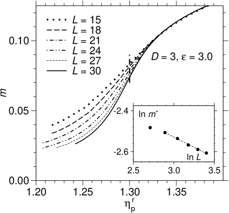
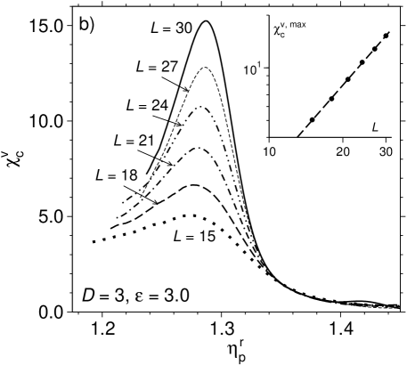
Figure 7: (a) Order parameter $m$ plotted versus $\eta_{\rm p}^{\rm r}$ for $D=3$, $\varepsilon=3.0$, and various choices of $L$ as indicated in the figure. At $\eta_{\rm p,crit}^{\rm r}$ (indicated by a vertical dashed line) the resulting data are shown in a log-log plot versus $L$ in the insert (the broken straight line indicates an effective exponent $(\beta/\gamma)_{\textrm{eff}}\approx 0.2$). (b) Susceptibility $\chi_{\rm c}$ plotted versus $\eta_{\rm p}^{\rm r}$ , for the same choices as in (a). Insert shows the maxima on a log-log plot vs. $L$ (broken straight line indicates an exponent $(\gamma/\nu)_{\textrm{eff}}\approx 1.6)$.

Figure 7a shows simulation results for the order parameter $m=(\eta_{\rm c}^{\ell}-\eta_{\rm c}^{v})/2$, where the volume fractions of colloids $\eta_{\rm c}^{\ell}$, $\eta_{\rm c}^{v}$ are not read off from the peak positions in Fig. 6a, since for shallow peaks this would be a somewhat arbitrary procedure, but rather we take $m$ as the first moment of the absolute value $\langle|M|\rangle$. Similarly, Fig. 7b shows the “susceptibility” $\chi_{0}=L^{2}D(\langle M^{2}\rangle-\langle|M|\rangle^{2})$. Both quantities are very strongly affected by finite size effects: Rather than exhibiting a power law decay, $m\propto(1-\eta_{\rm p,crit}^{\rm r}/\eta_{\rm p}^{\rm r})^{\beta}$ with $\beta=1/8$, one finds that approaching $\eta_{\rm p,crit}^{\rm r}$ from above, the curves for $m$ for the different values of $L$ splay out and develop very pronounced “finite size tails” 80 ; 95 for $\eta_{\rm p}^{\rm r}<\eta_{\rm p,crit}^{\rm r}$. At $\eta=\eta_{\rm p,crit}^{\rm r}$ one finds that the data are compatible with a power law decay (insert to Fig. 7a)

$$m^{*}(L)\equiv m(L,\eta_{\rm p,crit}^{\rm r})\propto L^{-\beta/\nu}\;.$$ (16)

According to the two-dimensional Ising model, one would expect $\beta/\nu=1/8$. However, the straight line in the insert of Fig. 7a rather indicates an effective exponent of $(\beta/\nu)_{\textrm{eff}}\approx 0.20\pm 0.02$. Likewise, the susceptibility maxima, which should scale as 80 ; 81 ; 82

$$\chi_{\rm c}^{\textrm{max}}\propto L^{\gamma/\nu}\;,$$ (17)

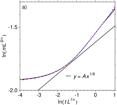
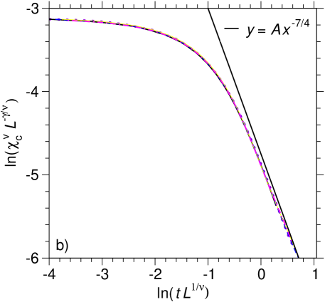
Figure 8: Scaling plot of the order parameter (a) and the susceptibility (b), using the three largest values of $L$ in Fig. 7, and the effective exponents (omitting here the index “eff”) $1/\nu=1.035,\beta/\nu=0.2$, and $\gamma/\nu=1.675$. The straight lines indicate the theoretical slope of the scaling functions for large values of $tL^{1/\nu}$, namely $\beta=1/8$ (a) and $\gamma=7/4$ (b).

with the two-dimensional Ising value being $\gamma/\nu=1.75$, rather suggest an effective exponent $(\gamma/\nu)_{\textrm{eff}}=1.60\pm 0.03$. Very roughly, these exponents are compatible with the hyperscaling relation 34 $\gamma/\nu+2\beta/\nu=2$. Using the quoted effective exponents $1/\nu_{\rm eff}$, $(\beta/\nu)_{\textrm{eff}}$ and $(\gamma/\nu)_{\textrm{eff}}$, one finds that on a scaling plot, where the variable $t\equiv|\eta_{\rm p,crit}^{\rm r}/\eta_{\rm p}^{\rm r}-1|$ is rescaled with $L^{1/\nu}$ and $m$ or $\chi$ are rescaled with $L^{\beta/\nu}$ or $L^{-\gamma/\nu}$, one finds reasonable data collapse (Fig. 8). Such a partial success of a finite size scaling analysis, i.e. good data collapse is only found when effective exponents are used that deviate somewhat from the theoretical values, has already been seen for interface localization-delocalization transitions in the Ising model 73 ; 74 and hence these problems are not a surprise in the present case.

IV OVERVIEW OF THE PHASE BEHAVIOR

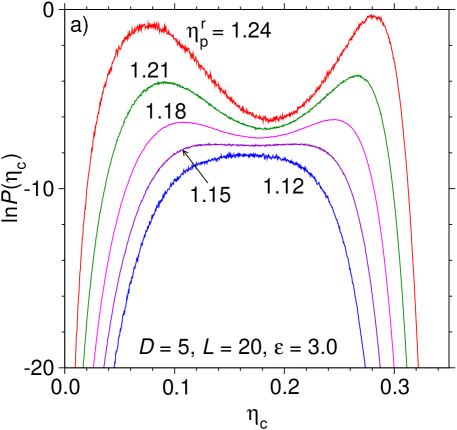
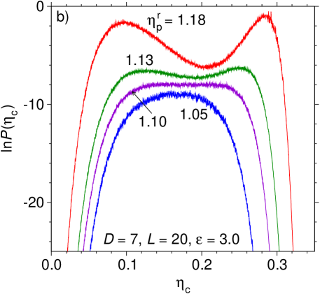
Figure 9: (a) Logarithm of the probability distribution of the colloid volume fraction, $\ln P(\eta_{\rm c})$, plotted vs. $\eta_{\rm c}$ for $D=5$, $L=20$, $\epsilon=3.0$, and four choices of $\eta_{\rm p}^{\rm r}$, as indicated. (b) Same as (a), but for $D=7$.

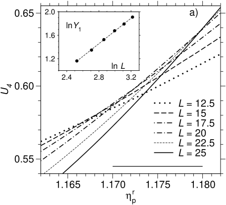
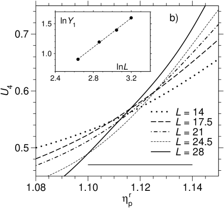
Figure 10: Cumulant $U_{4}$ plotted vs. $\eta_{\rm p}^{\rm r}$ for various choices of $L$ as indicated, for $\varepsilon=3.0$ and the film thickness $D=5$ (a) and $D=7$ (b). Inserts show plots of $\ln Y_{1}$ vs. $\ln L$, where $Y_{1}=\partial U_{4}/\partial\eta_{\rm p}^{\rm r}$. The broken straight lines indicate the effective exponent $(1/\nu)_{\textrm{eff}}$, with (a) $(1/\nu)_{\textrm{eff}}\approx 1.08$ and (b) $(1/\nu)_{\textrm{eff}}\approx 1.23$. The horizontal straight lines indicate the accuracy, with which $\eta_{\rm p,crit}^{\rm r}(D)$ can be estimated, namely $\eta_{\rm p,crit}^{\rm r}(D=5)=1.175\pm 0.005$ and $\eta_{\rm p,crit}^{\rm r}(D=7)=1.12\pm 0.02$.

We now describe some of our results for other film thicknesses $D$. In principle, the same type of analysis was carried out for $D=5$ and $D=7$ as well, but it turned out that the distribution $P(\eta_{\rm c})$ for $\eta_{\rm c}>\eta_{\rm c,crit}(D)$ becomes increasingly asymmetric when $D$ gets larger (Fig. 9). Also the cumulant intersections get spread out over a rather large range of $\eta_{\rm p}^{\rm r}$ (Fig. 10), and these intersection points lie even in a range that is below the three-dimensional Ising value, Eq. (14). We interpret this finding as an indication that with $D$ getting larger an increasing fraction of the critical region falls into the region of mean-field like behavior, as was theoretically predicted 74 .

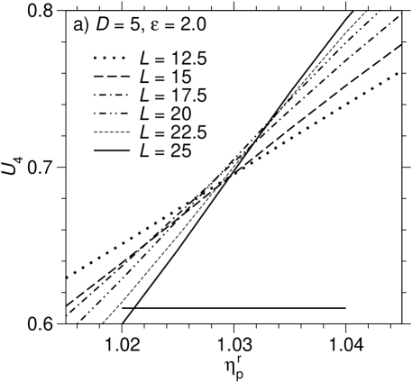
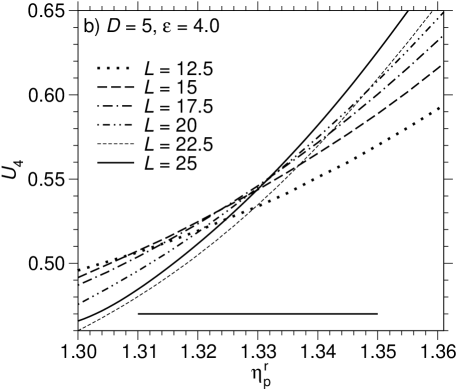
Figure 11: Cumulant $U_{4}$ plotted vs. $\eta_{\rm p}^{\rm r}$ for various choices of $L$ as indicated, for film thickness $D=5$ and two choices of $\epsilon$, $\varepsilon=2.0$ (a) and $\varepsilon=4.0$ (b). The horizontal straight lines indicate the accuracy with which $\eta_{\rm p,crit}^{\rm r}(D=5)$ can be estimated, namely $\eta_{\rm p,crit}^{\rm r}=1.03\pm 0.01$ ($\varepsilon=2.0$) and $\eta_{\rm p,crit}^{\rm r}=1.33\pm 0.02$ ($\varepsilon=4$).

Also for fixed $D$ the accuracy, with which $\eta_{\rm p,crit}^{\rm r}(D)$ can be estimated, clearly deteriorates when $\varepsilon$ increases (Fig. 11). Note that data for $D=5$ and $\varepsilon=1.0$ were already given in our preliminary communication 68 , the choice $\varepsilon=1.0$ corresponds to a capillary condensation-type behavior, however.

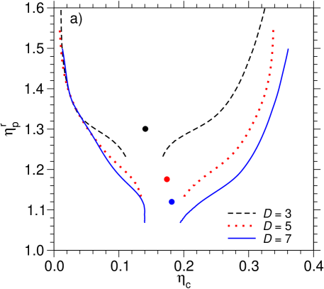
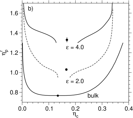
Figure 12: Phase diagrams in the plane of variables $\eta_{\rm p}^{\rm r}$ and $\eta_{\rm c}$ for the case $L=30$, $\varepsilon=3.0$, and three choices of $D$, $D=3$, 5, and 7 (a), as well as for the case $D=5$, $L=30$ and several choices of $\varepsilon$ (b). The full curves show the estimates for the binodal, while the filled circles represent the estimates of the critical points. In case (b), the estimate for the bulk coexistence curve (extrapolated towards $L\rightarrow\infty$) is included.

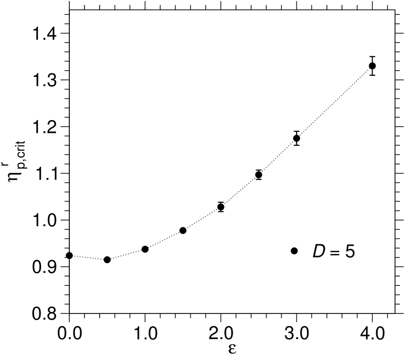
Figure 13: Plot of $\eta_{\rm p,crit}^{\rm r}(D=5)$ vs. $\epsilon$.

Figure 12a shows estimates for the phase diagrams for the interface localization transition for $\varepsilon=3$ and three choices of $D$, while Fig. 12b shows analogous data for $D=5$ but varying $\varepsilon$, and Fig. 13 shows a plot of $\eta_{\rm p,crit}^{\rm r}(D=5)$ vs. $\varepsilon$. One sees that miscibility is enhanced if either $D$ decreases, or $\varepsilon$ increases, or both.

Finally we turn to the variation of $\eta_{\rm p,crit}^{\rm r}$ with $\varepsilon$ for the choice $D=5$ (Fig. 13). As found from a self-consistent field calculation for a symmetrical polymer mixture confined between competing walls 77 , the minimum of the curve $\eta_{\rm p,crit}^{\rm r}$ does not occur for the case of symmetric walls ($\varepsilon=0$), but for an asymmetric situation. It also is remarkable and unexpected, that for large $\varepsilon$ the curve for $\eta_{\rm p,crit}^{\rm r}$ does not level off.

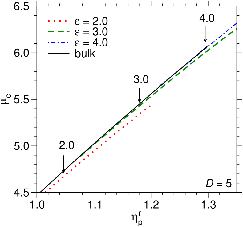
Figure 14: Plot of the colloid chemical potential versus $\eta_{\rm p}^{\rm r}$. The coexistence curve for asymmetric thin films, for $D=5$ and three values of $\varepsilon$, $\varepsilon=2.0,3.0$ and 4.0, as indicated, are compared to the coexistence curve of the colloid-polymer mixture in the bulk (solid line). Arrows show the critical points $\eta_{\rm p,crit}^{\rm r}(D)$. Note that the bulk critical point $(\eta_{\rm p,crit}^{\rm r}=0.766)$ is far beyond the scale of the diagram. For $\eta_{\rm p}^{\rm r}<\eta_{p,\textrm{crit}}^{r}(D)$ the meaning of the shown curves denotes the coexistence of domains in the stratified structure, with a single interface parallel to the walls, located via the maximum of $\langle M^{2}\rangle$.

Figure 14 shows the counterpart of the schematic Fig. 1 (left part), presenting in the plane of variables $\mu_{\rm c}$ and $\eta_{\rm p}^{\rm r}(D)$ the numerical results for the coexistence curves between colloid-rich and polymer-rich phases, for the case of $2.0\leq\varepsilon\leq 4.0$, i.e. the region where interface-localization transitions occur (which are highlighted in the diagram by arrows). Note that unlike Fig. 1, $\mu_{\rm c}(\infty)$ was not subtracted from $\mu_{\rm c}$, thus the bulk coexistence is not simply the ordinate axis as in Fig. 1, but rather a nontrivial curve (which actually is not very different from a straight line). While for $\varepsilon=2.0$ there is still a small but systematic offset between the curves $\mu_{\rm c}(\eta_{\rm p}^{\rm r},D=5)$ and $\mu_{\rm c}(\infty)$, for $\varepsilon=3.0$ and $\varepsilon=4.0$ the offset is almost negligibly small. The part of the curves $\mu_{\textrm{coex}}(\eta_{\rm p}^{\rm r}(D))$ to the left of $\eta_{\rm p,crit}^{\rm r}(D)$ represents the state BI in the schematic phase diagram, Fig. 1, where a delocalized interface occurs in the center of the film, separating the colloid-rich phase adjacent to the left wall and the polymer-rich phase adjacent to the right wall.

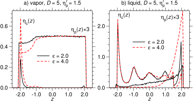
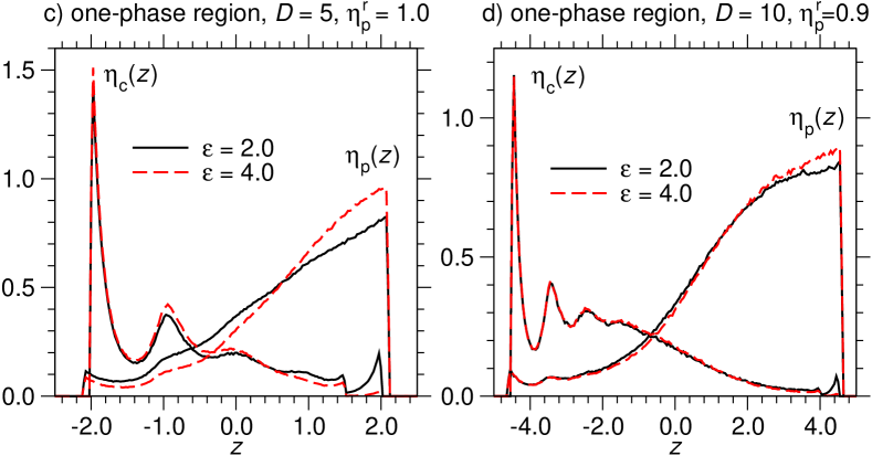
Figure 15: Comparison of the density profiles of colloids and polymers in the coexisting vapor-like phase (a) and liquid-like phase (b) between the cases $\varepsilon=2.0$ and 4.0, for $\eta_{\rm p}^{\rm r}=1.5$ and $D=5$. Panels c) and d) show the comparison of the density profiles of colloids and polymers between the cases $\epsilon=2.0$ and 4.0, but for the one-phase region in the “soft mode” phase. Panel c) displays the profiles for $D=5$ and $\eta_{\rm p}^{\rm r}=1.0$, panel d) the ones for $D=10$ and $\eta_{\rm p}^{\rm r}=0.9$.

At this point, we return to the density profiles at phase coexistence, and compare them for the same choice of $\eta_{\rm p}^{\rm r}$ and $D=10$, but different values of $\varepsilon$, $\varepsilon=2.0$ and $\varepsilon=4.0$ (Fig. 15). For $\eta_{\rm p}^{\rm r}=1.5$, the vapor-like phase reaches the same polymer density for both choices of $\varepsilon$; the main difference concerns the colloid-rich side of the systems, the colloid enrichment at the hard wall is more pronounced for $\varepsilon=4.0$ than for $\varepsilon=2.0$. However, in the liquid-like colloid-rich phase the behavior is just the other way round: the layered profiles of the colloid-rich phase near the hard all are virtually identical, while the polymer enrichment near the right wall is more pronounced for $\varepsilon=4.0$ than for $\varepsilon=2.0$. When one studies the effect of varying $\varepsilon$ in the one phase region for $\eta_{\rm p}^{\rm r}<\eta_{\rm p,crit}^{\rm r}(D)$ however, one sees only a minor effect of $\varepsilon$ on the segregated structure where an interface has formed parallel to the walls (Fig. 15b and 15d), in particular for not extremely thin films.

V CONCLUSIONS

In this paper, the Asakura-Oosawa (AO) model for colloid-polymer mixtures for a size ratio of polymers to colloids $q=0.8$ was studied by Monte Carlo simulation, considering thin films of thickness $D=3$ to $D=10$ colloid diameters and confinement between asymmetric walls. One wall is simply a repulsive hard wall, to which the colloidal particles are attracted via depletion forces; the other wall exerts a square-well-type repulsive interaction (of the range of the colloid ratio, and variable strength $\varepsilon=0.5$ to 4.0, in units of $k_{B}T=1.0$). This study complements our earlier work on the AO model in the bulk, and under confinement between two equivalent hard walls, where capillary-condensation like phenomena occur; for the present model, we can smoothly interpolate from capillary condensation-like behavior for small $\varepsilon$ (e.g. $\varepsilon=0.5$ or 1.0), when both walls show some (though unequal) surface enrichment of colloids, to interface localization-type transitions, occurring for large $\varepsilon$ (e.g. for $\varepsilon$ varying from $\varepsilon=2.5$ to $\varepsilon=4.0$). In the latter case, only the hard wall attracts colloids while the other wall attracts polymers. In this region, for large $D$ the precise value of $\varepsilon$ has little effect on the observed density profiles. When one then increases the polymer reservoir packing fraction $\eta_{\rm p}^{\rm r}$ (which plays an analogous role as the inverse temperature does for thermally driven phase separation in small molecules mixtures), one observes that the enrichment layers of colloids and polymers at the walls gradually transform into two domains of coexisting colloid-rich and polymer-rich phases, separated by an interface parallel to the confining walls. We find that the temperature dependence of the width of this interface is considerably weaker than that of the bulk correlation length (or “intrinsic” interfacial width, respectively), and account for this finding in terms of capillary wave broadening of the interface. However, since for $D<10$ the interface profiles are strongly affected by layering of colloids near the hard wall, study of this broadening is difficult.

Only far away from the bulk critical point can a sharp phase transition be observed, which we analyze by finite size scaling methods. While for $D=3$ and not too large $\varepsilon$ the critical value $\eta_{\rm p,crit}^{\rm r}(D)$ can be rather accurately determined, and evidence can be found that the critical behavior falls in the universality class of the two-dimensional Ising model, for larger $D$ and/or larger $\varepsilon$ the Monte Carlo data are strongly affected by problems of crossover between different universality classes and, thus, $\eta_{\rm p,crit}^{\rm r}(D)$ can be only estimated with rather modest accuracy, allowing no firm statements about critical exponents. Approaching the transition from $\eta_{\rm p}^{\rm r}<\eta_{\rm p,crit}^{\rm r}(D)$, we find a strong increase of the correlation length $\xi_{||}$ describing the correlation of interfacial fluctuations, but again the accuracy of our results would not suffice to estimate the value of the associated critical exponent. In view of the fact that even for the simple Ising model confined between competing boundaries a clarification of the critical behavior turned out to be very difficult, the problems encountered for the present more complicated model, which is strongly asymmetric even in the bulk, are not at all surprising.

The fact that observation of interface localization does not require very special conditions at the walls, but occurs for a broad parameter range, is encouraging for possible experimental tests of our results. We suggest that a repulsive interaction acting only on the colloids could be realized by creating a wall with a polymer brush at low grafting density.

A very interesting problem, not accessible to the present grand-canonical Monte Carlo study, would be the dynamics of phase separation in such a confined thin film. We hope to report on such studies of a related model in the future.

Acknowledgments: This work was supported in part by the Deutsche Forschungsgemeinschaft, SFB TR6/A5 and C3.

References

- (1) J. S. Rowlinson and B. Widom, Molecular Theory of Capillarity (Oxford University Press, London, 1982).
- (2) C. A. Croxton (ed.), Fluid Interfacial Phenomena (Wiley, New York, 1985).
- (3) J. Charvolin, J.-F. Joanny, and J. Zinn-Justin (eds.), Liquids at Interfaces (North-Holland, Amsterdam, 1990).
- (4) D. Henderson (ed.), Fundamentals of Inhomogeneous Fluids (Dekker, New York, 1992).
- (5) R. Evans, J. Phys.: Condens. Matter 2, 8989 (1990).
- (6) L. D. Gelb, K. E. Gubbins, R. Radhakrishnan, and M. Sliwinska-Bartkowiak, Rep. Prog. Phys. 62, 1573 (1999).
- (7) K. Binder, D. P. Landau, and M. Müller, J. Stat. Phys. 110, 1411 (2003).
- (8) M. Schön and S. Klapp, Rev. Comp. Chem., Vol. 24 (Wiley-VCH, Hoboken, 2007).
- (9) K. Binder, J. Horbach, R. Vink, and A. De Virgiliis, Soft Matter 4, 1555 (2008).
- (10) K. Binder, Ann. Rev. Mat. Sc. (2008, in press).
- (11) E. L. Wolf, Nanophysics and Nanotechnology (Wiley-VCH, Weinheim, 2004).
- (12) R. W. Kelsall, I. W. Hamley, and M. Geoghegan (eds.), Nanoscale Science and Technology (Wiley-VCH, Weinheim, 2005).
- (13) H. Watarai, Interfacial Nanochemistry: Molecular Science and Engineering at Liquid-Liquid Interfaces (Springer, Berlin, 2005).
- (14) A. Meller, J. Phys.: Condens. Matter 15, R581 (2003).
- (15) T. M. Squires and S. R. Quake, Rev. Mod. Phys. 77, 977 (2005).
- (16) M. Koza, B. Frick, and R. Zorn (eds.), 3rd International Workshop on Dynamics in Confinement, Eur. Phys. J. ST 141, (2007).
- (17) S. J. Gregg and K. S. W. Sing, Adsorption, Surface Area, and Porosity, 2nd ed. (Academic, New York, 1982).
- (18) F. Rouquerol, J. Rouquerol, and K. S. W. Sing, Adsorption by Powders and Porous Solids: Principles, Methodology and Applications (Academic, San Diego, 1999).
- (19) F. Schüth, K. S. W. Sing, and J. Weitkamp (eds), Handbook of Porous Solids (Wiley-VCH, Weinheim, 2002).
- (20) W. C. K. Poon and P. N. Pusey, in Observation, Prediction, and Simulation of Phase Transitions in Complex Fluids, edited by M. Baus, L. F. Rull, and J. P. Ryckaert (Kluwer Academic, Dordrecht, 1995), p. 3.
- (21) A. K. Arora and B. V. R. Tata, Adv. Coll. Int. Sci. 78, 49 (1998).
- (22) H. Löwen, J. Phys.: Condens. Matter 13, R415 (2001).
- (23) W. C. K. Poon, J. Phys.: Condens. Matter 14, R589 (2002).
- (24) W. C. K. Poon, Science 304, 830 (2004).
- (25) A. van Blaaderen, Prog. Colloid Polym. Sci. 104, 59 (1997).
- (26) A. P. Gast, C. K. Hall, and W. B. Russel, J. Coll. Int. Sci. 96, 251 (1983).
- (27) S. Asakura and F. Oosawa, J. Chem. Phys. 22, 1255 (1954); J. Polym. Sci. 33, 183 (1958).
- (28) A. Vrij, Pure App. Chem. 48, 471 (1976).
- (29) H. Lekkerkerker, W. C. K. Poon, P. N. Pusey, A. Stroobants, and P. B. Warren, Europhys. Lett. 20, 559 (1992).
- (30) M. Dijkstra and R. van Roij, Phys. Rev. Lett. 89, 208303 (2002).
- (31) M. Schmidt, A. Fortini, and M. Dijkstra, J. Phys.: Condens. Matter 15, S3411 (2003).
- (32) R. L. C. Vink and J. Horbach, J. Chem. Phys. 121, 3253 (2004); J. Phys.: Condens. Matter 16, S3807 (2004).
- (33) R. L. C. Vink, J. Horbach, and K. Binder, Phys. Rev. E 71, 011401 (2005).
- (34) M. E. Fisher, Rev. Mod. Phys. 46, 597 (1974).
- (35) J. M. Brader, R. Evans, M. Schmidt, and H. Löwen, J. Phys.: Condens. Matter 14, L1 (2002).
- (36) P. G. de Gennes, Rev. Mod. Phys. 57, 827 (1985).
- (37) D. E. Sullivan and M. M. Telo da Gama, in Ref. 2 , p. 45.
- (38) S. Dietrich in Phase Transitions and Critical Phenomena, edited by C. Domb and J. L. Lebowitz (Academic, New York, 1988), Vol. XII, p. 1
- (39) M. Schick, in Ref. 3 , p. 415.
- (40) D. Bonn and D. Ross, Rep. Prog. Phys. 64, 1085 (2001).
- (41) W. K. Wijting, N. A. M. Besseling, and M. A. Cohen Stuart, Phys. Rev. Lett. 90, 196101 (2003).
- (42) D. G. A. L. Aarts, R. P. A. Dullens, D. Bonn, R. van Roij, and H. N. W. Lekkerkerker, J. Chem. Phys. 120, 1973 (2004).
- (43) D. G. A. L. Aarts, J. Phys. Chem. B 109, 7407 (2005).
- (44) M. Dijkstra, R. van Roij, R. Roth, and A. Fortini, Phys. Rev. E 73, 041404 (2006).
- (45) A. Fortini, M. Schmidt, and M. Dijkstra, Phys. Rev. E 73, 051502 (2006).
- (46) Y. Hennequin, D. G. A. L. Aarts, J. O. Indekeu, H. N. W. Lekkerkerker, and D. Bonn, Phys. Rev. Lett. 100, 178305 (2008).
- (47) G. A. Vliegenthart and H. N. W. Lekkerkerker, Prog. Coll. Pol. Sc. 105, 27 (1997).
- (48) E. H. A. de Hoog and H. N. W. Lekkerkerker, J. Phys. Chem. B 103, 5274 (1999).
- (49) B. H. Chen, B. Payandeh, and M. Robert, Phys. Rev. E 62, 2369 (2000).
- (50) R. L. C. Vink, J. Horbach, and K. Binder, J. Chem. Phys. 112, 134905 (2005).
- (51) M. von Smoluchowski, Ann. Phys. (Leipzig) 25, 205 (1908).
- (52) L. Mandelstam, Ann. Phys. (Leipzig) 41, 608 (1913).
- (53) F. P. Buff, R. Lovett, and F. H. Stillinger, Phys. Rev. Lett. 15, 621 (1965).
- (54) J. D. Weeks, J. Chem. Phys. 67, 3106 (1977); Phys. Rev. Lett. 15, 2160 (1984).
- (55) V. Privman, Int. J. Mod. Phys. C 3, 857 (1992).
- (56) D. G. A. L. Aarts, M. Schmidt, and H. N. W. Lekkerkerker, Science 304, 847 (2004).
- (57) M. Schmidt, A. Fortini, and M. Dijkstra, J. Phys.: Condens. Matter 15, S3411 (2003).
- (58) R. L. C. Vink, K. Binder, and J. Horbach, Phys. Rev. E 73, 056118 (2006).
- (59) R. L. C. Vink, A. De Virgiliis, J. Horbach, and K. Binder, Phys. Rev. E 74, 031601 (2006); Erratum, Phys. Rev. E 74, 069903 (2006).
- (60) M. E. Fisher and H. Nakanishi, J. Chem. Phys. 75, 5857 (1981).
- (61) A. Patrykiejew, S. Sokolowski, and K. Binder, Surf. Sc. Rep. 37, 207 (2000).
- (62) J. L. Salamacha, A. Patrykiejew, S. Sokolowski, and K. Binder, J. Chem. Phys. 122, 074703 (2005).
- (63) D. H. Napper, Polymeric Stabilization of Colloidal Dispersions (Academic, London, 1983).
- (64) R. C. Advincula, W.-J. Brittain, R. C. Carter, and J. Rühe (eds.), Polymer Brushes (Wiley-VCH, Weinheim, 2004).
- (65) A. Halperin, M. Tirrell, and T. P. Lodge, Adv. Pol. Sci. 100, 31 (1991).
- (66) T. Kerle, R. Yerushalmi-Rozen, and J. Klein, Europhys. Lett. 38, 207 (1997).
- (67) G. Reiter and R. Khanna, Phys. Rev. Lett. 85, 5599 (2000).
- (68) A. De Virgiliis, R. L. C. Vink, J. Horbach, and K. Binder, Europhys. Lett. 77, 60002 (2007).
- (69) E. V. Albano, K. Binder, D. W. Heermann, and W. Paul, Surf. Sci. 223, 151 (1989).
- (70) A. O. Parry and R. Evans, Phys. Rev. Lett. 64, 439 (1990).
- (71) M. R. Swift, A. L. Owczarek, and J. O. Indekeu, Europhys. Lett. 14, 475 (1991).
- (72) A. O. Parry and R. Evans, Physica A 181, 250 (1992).
- (73) K. Binder, D. P. Landau, and A. M. Ferrenberg, Phys. Rev. Lett. 74, 298 (1995); Phys. Rev. E 51, 2823 (1995).
- (74) K. Binder, R. Evans, D. P. Landau, and A. M. Ferrenberg, Phys. Rev. E 53, 5023 (1996).
- (75) M. Müller, K. Binder, and E. V. Albano, Physica A 279, 188 (2000).
- (76) M. Müller, E. V. Albano, and K. Binder, Phys. Rev. E 62, 5281 (2000).
- (77) M. Müller, K. Binder and E. V. Albano, Europhys. Lett. 50, 724 (2000).
- (78) M. Müller and K. Binder, Phys. Rev. E 63, 021602 (2001).
- (79) P. Virnau and M. Müller, J. Chem. Phys. 120, 10925 (2004).
- (80) K. Binder, Z. Phys. B 43, 119 (1981); Rep. Prog. Phys. 60, 487 (1997).
- (81) M. E. Fisher, in Critical Phenomena, ed. by M. S. Green (Academic, London, 1971), p. 1.
- (82) V. Privman (ed.), Finite Size Scaling and Numerical Simulation of Statistical Systems (World Scientific, Singapore, 1990).
- (83) A. Werner, F. Schmid, M. Müller, and K. Binder, J. Chem. Phys. 107, 8175 (1997).
- (84) K. Binder, M. Müller, F. Schmid, and A. Werner, J. Stat. Phys. 95, 1045 (1999).
- (85) T. Kerle, J. Klein, and K. Binder, Phys. Rev. Lett. 77, 1318 (1996); Eur. Phys. J. B 7, 401 (1999).
- (86) P. G. de Gennes, Scaling Concepts iin Polymer Physics (Cornell University Press, Ithaca, N. Y., 1979).
- (87) K. Binder, Adv. Pol. Sc. 138, 1 (1999).
- (88) B. Widom, in Phase Transitions and Critical Phenomena, ed. by C. Domb and M. S. Green, Vol. 2, (Academic, London, 1972), p. 79.
- (89) D. Jasnow, Rep. Prog. Phys. 47, 1059 (1984).
- (90) E. Brezin, B. I. Halperin, and S. Leibler, Phys. Rev. Lett. 50, 1387 (1983).
- (91) R. Lipowsky, D. M. Kroll, and R. K. P. Zia, Phys. Rev. B 27, 4499 (1983).
- (92) M. E. Fisher and H. Wen, Phys. Rev. Lett. 68, 3654 (1992).
- (93) A. O. Parry, J. M. Romero-Enrique, and A. Lazarides, Phys. Rev. Lett. 93, 086104 (2004).
- (94) A. M. Ferrenberg and R. H. Swendsen, Phys. Rev. Lett. 61, 2635 (1988); 63, 1195 (1989).
- (95) K. Binder and D. P. Landau, Phys. Rev. B 30, 1477 (1984).
- (96) C. Borgs and R. Kolecky, J. Stat. Phys. 61, 79 (1990).
- (97) D. P. Landau and K. Binder, A Guide to Monte Carlo Simulation in Statistical Physics (Cambridge University Press, Cambridge, 2005).
- (98) G. Kamieniarz and H. W. J. Blöte, J. Phys. A 26, 201 (1993).
- (99) N. Wilding, in Annual Reviews of Computational Physics, edited by D. Stauffer (World Scientific, Singapore, 1996) p. 37.