Deriving Boltzmann Equations from Kadanoff–Baym Equations
in Curved Space–Time

Abstract

To calculate the baryon asymmetry in the baryogenesis via leptogenesis scenario one usually uses Boltzmann equations with transition amplitudes computed in vacuum. However, the hot and dense medium and, potentially, the expansion of the universe can affect the collision terms and hence the generated asymmetry. In this paper we derive the Boltzmann equation in the curved space-time from (first-principle) Kadanoff–Baym equations. As one expects from general considerations, the derived equations are covariant generalizations of the corresponding equations in Minkowski space-time. We find that, after the necessary approximations have been performed, only the left-hand side of the Boltzmann equation depends on the space-time metric. The amplitudes in the collision term on the right–hand side are independent of the metric, which justifies earlier calculations where this has been assumed implicitly. At tree level, the matrix elements coincide with those computed in vacuum. However, the loop contributions involve additional integrals over the the distribution function.

I Introduction

As has been shown by A. Sakharov Sakharov (1967), the observed baryon asymmetry of the universe can be generated dynamically, provided that the following three conditions are fulfilled: violation of baryon (or baryon minus lepton) number; violation of C and CP; and deviation from thermal equilibrium.

The third Sakharov condition raises the question of how to describe a quantum system out of thermal equilibrium. The usual choice is the Boltzmann equation Bernstein (1988); de Groot et al. (1980); Cercignani and Kremer (2002); Liboff (2003). However, it is known to have several shortcomings. In particular classical Boltzmann equations neglect off–shell effects, introduce irreversibility and feature spurious constants of motion. A quantum mechanical generalization of the Boltzmann equation, free of the mentioned problems, has been developed by L. Kadanoff and G. Baym Kadanoff and Baym (1962). Direct numerical computations demonstrate that already for simple systems far from thermal equilibrium the Kadanoff–Baym and Boltzmann equations do lead to quantitatively, and in some cases even qualitatively, different results Berges (2002); Aarts and Berges (2001); Lindner and Muller (2006, 2008); Berges et al. (2005a); Juchem et al. (2004). Studying processes responsible for the generation of the asymmetry in the framework of the Kadanoff–Baym formalism is therefore of considerable scientific interest.

The application of the Kadanoff–Baym equations to the computation of the lepton and baryon asymmetries in the leptogenesis scenario Fukugita and Yanagida (1986) has been studied at different levels of approximation by several authors Buchmuller and Fredenhagen (2000); De Simone and Riotto (2007) and lead to qualitatively new and interesting results. However issues related to the rapid expansion of the universe, which drives the required deviation from thermal equilibrium, have not been addressed there. The modification of the Kadanoff–Baym formalism in curved space–time has been considered in Calzetta and Hu (1987); Calzetta et al. (1988); Ramsey and Hu (1997); Tranberg (2008), where it was applied to a model with quartic self–interactions and a $O(N)$ model, though the dynamics of quantum field theoretical models with CP violation remained uninvestigated.

Our goal is to develop a consistent description of leptogenesis in the Kadanoff–Baym and Boltzmann approaches and to test approximations commonly made in the computation of the lepton and baryon asymmetries. In particular, we want to find out how the dense background plasma and the curvature of spacetime affect the collision terms of processes contributing to the generation and washout of the asymmetry, check the applicability of the real intermediate state subtraction procedure in the case of resonant leptogenesis Pilaftsis and Underwood (2004, 2005), and investigate the time dependence of the CP–violating parameter in the expanding universe De Simone and Riotto (2007).

Since this is a rather ambitious goal, we first study a simple toy model of leptogenesis containing two real and one complex scalar fields, which mimic the heavy right–handed Majorana neutrinos and leptons respectively Garny et al. (2009a). The peculiarities of the calculation, related to the presence of a gravitational field, are determined only by transformation properties of the quantum fields – scalar fields in this case. For this reason, in the present paper, we use a model of a single real scalar field with quartic self–interactions, minimally coupled to gravity, to illustrate the main points. That is, we use the Lagrangian

$${\cal L}=\frac{1}{2}\partial^{\mu}\varphi\partial_{\mu}\varphi-\frac{1}{2}M^{2}\varphi^{2}-\frac{\lambda}{4!}\varphi^{4}\,,$$ (1)

which does also have the advantage, that one can compare the derived equations with their Minkowski space–time counterparts Lindner and Muller (2006) and with the results obtained in Calzetta and Hu (1987); Calzetta et al. (1988); Ramsey and Hu (1997); Tranberg (2008). The formalism presented here will be used to analyze the toy model of leptogenesis.

The starting point of our analysis, which is manifestly covariant in every step, is the generating functional for the (connected) Green’s functions. Performing a Legendre transformation we get the effective action, which we use to derive the Schwinger–Dyson equations in Sec. II. These are equivalent to a system of Kadanoff–Baym equations for the spectral function and the statistical propagator, which we derive in Sec. IV. Employing a first–order gradient expansion and a Wigner transformation we are lead to a system of quantum kinetic equations which we study in Sec. V. Finally, neglecting the Poisson brackets and making use of the quasiparticle approximation, we obtain the Boltzmann equation in Sec. VI.

• The Kadanoff–Baym equations and the derived Boltzmann equation are covariant generalizations of their Minkowski–space counterparts.

• The space-time metric enters its left-hand side in the form of the covariant derivative, whereas the collision terms on the right-hand side are independent of the metric.

• At tree-level the collision terms coincide with those calculated in vacuum, whereas the loop corrections contain integrals over the distribution function.

• In the loop contributions one can clearly distinguish the initial, final and on–shell intermediate states, which is not the case in the canonical formalism.

We discuss these results in more details and draw the conclusions in Sec. VII.

II Schwinger–Dyson equations

In the derivation of the Schwinger-Dyson equations we employ results from Ramsey and Hu (1997); Basler (1993); Toms (1987). Our starting point is the generating functional for Green’s functions with local and bi–local external scalar sources $J(x)$ and $K(x,y)$,

$${\cal Z}[J,K]={\textstyle\int}\mathscr{D}\varphi~{}\exp[i(S+J\varphi+{\textstyle\frac{1}{2}}\varphi K\varphi)],$$ (2)

where the action $S$ is given by the integral of the Lagrange density over space. The Minkowski space–time volume element $d^{4}x$ is replaced in curved space–time by the invariant volume element $\sqrt{-g}d^{4}x$, where $\sqrt{-g}$ is the square root of the determinant of the metric:

$$S ={\textstyle\int}\sqrt{-g}d^{4}x~{}{\cal L}\,.$$

In the Friedmann–Robertson–Walker (FRW) universe we have $\sqrt{-g}=a^{4}(\eta)$, where $a$ is the scale factor and $\eta$ denotes conformal time. The invariant volume element enters also in the scalar products of the sources and the field

$$J\varphi \equiv{\textstyle\int}\sqrt{-g}d^{4}xJ(x)\varphi(x)\,,$$ (3a)

$$\varphi K\varphi \equiv{\textstyle\iint}\sqrt{-g}d^{4}x\sqrt{-g}d^{4}y~{}\varphi(x)K(x,y)\varphi(y)\,.$$ (3b)

The functional integral measure is modified in curved space–time as well. For scalar densities of zero weight it reads Basler (1993)

$$\mathscr{D}\varphi=\prod_{x}d[(-g)^{\frac{1}{4}}\varphi(x)]\,.$$

The evolution of the quantum system out of thermal equilibrium is performed in the Schwinger–Keldysh formalism Schwinger (1961); Keldysh (1965). In this approach the field and the external sources are defined on the positive and negative branches of a closed real–time contour, see Fig. 1, the functions on the positive branch being independent of the functions on the negative branch. This applies also to the metric tensor, i.e. $g^{+}_{\mu\nu}\neq g^{-}_{\mu\nu}$ in general.

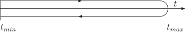
Figure 1: Closed real–time path $\cal C$.

In realistic models of leptogenesis the contribution of the heavy right–handed neutrinos to the energy density of the universe is less than 5% and can safely be neglected. In other words, leptogenesis takes place in a space–time with a metric, whose time development is (in this approximation) independent of the decays of the right–handed neutrinos and determined by the contributions of the ultrarelativistic standard model species. Correspondingly, in our analysis of the toy model of leptogenesis, we will also neglect the impact of the scalar fields on the expansion of the universe. This implies in particular that the metric tensor on the positive and negative branches is determined only by the external processes, and one can set $g^{+}_{\mu\nu}=g^{-}_{\mu\nu}=g_{\mu\nu}$. To shorten the notation we will also suppress the branch indices of the scalar field and the sources.

The existence of the two branches also affects the definition of the $\delta$ function: $\delta(x,y)$ is always zero if its arguments lie on different branches Danielewicz (1984). In curved space–time it is further generalized to fulfill the relation

$${{\textstyle\int}}d^{4}y\sqrt{-g}~{}f(y)~{}\delta^{g}(x,y)=f(x)\,,$$ (4)

where the integration is performed over the closed contour. The solution to this equation is given by Basler (1993)

$$\delta^{g}(x,y)=(-g_{x})^{-\frac{1}{4}}\delta(x,y)(-g_{y})^{-\frac{1}{4}}\,.$$ (5)

The generalized $\delta$ function is used to define functional differentiation in curved space–time Zaidi (1983)

$$\frac{\delta{\cal F}[\phi]}{\delta\phi(y)}\equiv\lim\limits_{\varepsilon\rightarrow 0}\frac{{\cal F}[\phi(x)+\varepsilon\,\delta^{g}(x,y)]-{\cal F}[\phi(x)]}{\varepsilon}\,.$$ (6)

From the definition (6) it follows immediately that

$$\frac{\delta J(x)}{\delta J(y)}=\delta^{g}(x,y)~{},\quad\frac{\delta K(x,y)}{\delta K(u,v)}=\delta^{g}(x,u)\delta^{g}(y,v)\,.$$ (7)

The functional derivatives of the generating functional for connected Green’s functions

$${\cal W}[J,K]=-i\ln{\cal Z}[J,K]\,$$ (8)

with respect to the external sources read

$$\frac{\partial{\cal W}[J,K]}{\partial J(x)} =\Phi(x)\,,$$ (9a)

$$\frac{\partial{\cal W}[J,K]}{\partial K(x,y)} ={\textstyle\frac{1}{2}}[G(y,x)+\Phi(x)\Phi(y)]\,,$$ (9b)

where $\Phi$ denotes expectation value of the field and $G$ is the propagator. The effective action is the Legendre transform of the generating functional for connected Green’s functions,

$$\Gamma[\Phi,G]\equiv{\cal W}[J,K]-J\Phi-{\textstyle\frac{1}{2}}{\rm tr}[KG]-{\textstyle\frac{1}{2}}\Phi K\Phi\,.$$ (10)

Its functional derivatives with respect to the expectation value and the propagator reproduce the external sources:

$$\frac{\delta\Gamma[G,\Phi]}{\delta\Phi(x)} =-J(x)-{\textstyle\int}\sqrt{-g}d^{4}z~{}K(x,z)\Phi(z)\,,$$ (11a)

$$\frac{\delta\Gamma[G,\Phi]}{\delta G(x,y)} =-{\textstyle\frac{1}{2}}K(y,x)\,.$$ (11b)

Next, we shift the field by its expectation value

$$\varphi\rightarrow\varphi+\Phi\,.$$

The action can then be written as a sum of two terms

$$S[\varphi]\rightarrow S_{cl}[\Phi]+S[\varphi,\Phi]\,.$$ (12)

$S_{cl}$ denotes the classical action, which depends only on $\Phi$, whereas $S[\varphi,\Phi]=S_{0}[\varphi]+S_{int}[\varphi,\Phi]$ contains terms quadratic, cubic and quartic in the shifted field $\varphi$. The free field action can be written in the form

$$S_{0}={\textstyle\frac{1}{2}\iint}\sqrt{-g}_{x}d^{4}x\sqrt{-g}_{y}d^{4}y\,\varphi\left(i\mathscr{G}^{-1}\right)\varphi\,,$$ (13)

where $\mathscr{G}^{-1}$ is the zero–order inverse propagator

$$\mathscr{G}^{-1}(x,y)=i(\square_{x}+M^{2})\,\delta^{g}(x,y),\,\square_{x}\equiv g_{\mu\nu}\nabla^{\mu}_{x}\nabla^{\nu}_{x}\,.$$ (14)

Since the integration measure in the path integral is translationally invariant, the effective action can be rewritten in the form

$$\Gamma[\Phi,G]= -i\ln{\textstyle\int}\mathscr{D}\varphi\exp[i(S+J\varphi+{\textstyle\frac{1}{2}}\varphi K\varphi)]$$

$$+S_{cl}[\Phi]-{\textstyle\frac{1}{2}}{\rm tr}[KG]\,.$$ (15)

Now we tentatively write the effective action in the form

$$\Gamma[\Phi,G] \equiv S_{cl}[\Phi]+{\textstyle\frac{i}{2}}\ln\det\left[G^{-1}\right]+{\textstyle\frac{i}{2}}{\rm tr}\left[\mathscr{G}^{-1}G\right]$$

$$\hskip 11.38092pt+\Gamma_{2}[\Phi,G]\,,$$ (16)

defining the functional $\Gamma_{2}$. The third term on the right–hand side is defined by

$${\rm tr}\left[\mathscr{G}^{-1}G\right]\equiv{\textstyle\iint}\sqrt{-g_{x}}d^{4}x\sqrt{-g_{y}}d^{4}y~{}\mathscr{G}^{-1}(x,y)G(y,x)\,,$$

whereas the second term on the right–hand side is defined by the path integral

$$\det\left[\frac{G^{-1}}{2\pi}\right]\equiv{\textstyle\int}\mathscr{D}\varphi\exp\left(\varphi\,{G^{-1}}\varphi\right)\,.$$

Using (11) we can find the functional derivatives of $\Gamma$. Differentiation of ${\rm tr}\left[\mathscr{G}^{-1}G\right]$ with respect to $G$ is straightforward and gives

$$\frac{\delta}{\delta G(x,y)}{\rm tr}\left[\mathscr{G}^{-1}G\right]=\mathscr{G}^{-1}(y,x)\,.$$ (17)

To calculate the functional derivative of $\ln\det\left[G^{-1}\right]$ we take into account that in curved space–time

$${\textstyle\int}\sqrt{-g}\,d^{4}z\,G^{-1}(u,z)G(z,v)=\delta^{g}(u,v)~{}.$$ (18)

After some algebra and use of (18) we obtain a result analogous to that in Minkowski space–time

$$\frac{\delta}{\delta G(x,y)}\ln\det\left[G^{-1}\right]=-G^{-1}(y,x)\,.$$ (19)

The functional derivative of (II) with respect to $G$ then reads

$$\frac{\delta\Gamma[G,\Phi]}{\delta G(x,y)}= -{\textstyle\frac{i}{2}}G^{-1}(y,x)+{\textstyle\frac{i}{2}}\mathscr{G}^{-1}(y,x)+\frac{\delta\Gamma_{2}[G,\Phi]}{\delta G(x,y)}$$

$$= -{\textstyle\frac{1}{2}}K(y,x)$$ (20)

Solving (II) with respect to $K$ and substituting it into (II) we can rewrite the effective action in the form

$$\Gamma_{2}[G ,\Phi]=-i\ln\int\mathscr{D}\varphi\exp\left[i\left(S+J\varphi-\varphi\frac{\delta\Gamma_{2}}{\delta G}\varphi\right)\right]$$

$$+{\rm tr}\left[\frac{\delta\Gamma_{2}}{\delta G}G\right]-{\textstyle\frac{i}{2}}\ln\det\left[G^{-1}\right]+const.\,,$$ (21)

where again $S=S_{0}+S_{int}$, but now with $S_{0}$ given by

$$S_{0}={\textstyle\frac{1}{2}\iint}\sqrt{-g}_{x}d^{4}x\sqrt{-g}_{y}d^{4}y\,\varphi\left(iG^{-1}\right)\varphi\,.$$ (22)

This implies that $i\Gamma_{2}$ is the sum of all 2PI vacuum diagrams with vertices as given by ${\cal L}_{int}$ and internal lines representing the complete connected propagators $G$ Cornwall et al. (1974).

Physical situations correspond to vanishing sources. Introducing the self–energy

$$\Pi(x,y)\equiv 2i\frac{\delta\Gamma_{2}[G,\Phi]}{\delta G(y,x)}\,,$$ (23)

we can then rewrite (II) in the form

$$G^{-1}(x,y)=\mathscr{G}^{-1}(x,y)-\Pi(x,y)\,.$$ (24)

Thus the above calculation yields the Schwinger–Dyson (SD) equation. Let us note that the derived equation has exactly the same form as in Minkowski space–time.

III 2PI effective action

The structure of the Schwinger–Dyson equation is determined only by the particle content of the model (here a single real scalar field) and completely independent of the particular form of the interaction Lagrangian. The latter determines the form of the 2PI effective action. The lowest order contribution is due to the two–loop diagram in Fig. 2,

Figure 2: Two–, three–, and four–loop contributions to the 2PI effective action.

which only takes into account local effects and cannot describe thermalization. Thus one usually also considers the three–loop diagram, which describes $2\leftrightarrow 2$ scattering. In addition we take into account the four–loop contribution. As is demonstrated below, in the Boltzmann approximation it describes the one–loop correction for $2\leftrightarrow 2$ scattering. The resulting expression for the effective action is similar to that given in Aarts and Berges (2001); Lindner and Muller (2006); Ramsey and Hu (1997); Berges (2004):

$$i\Gamma_{2}[G] =\sum\limits_{n}i\Gamma^{(n)}_{2}[G],$$ (25)

$$i\Gamma^{(2)}_{2}[G] =-\,\frac{i\lambda}{8}{\textstyle\int}\sqrt{-g}_{x}d^{4}x\,G^{2}(x,x),$$

$$i\Gamma^{(3)}_{2}[G] =-\,\frac{\lambda^{2}}{48}{\textstyle\int}\sqrt{-g}_{x}d^{4}x\sqrt{-g}_{y}d^{4}y\,G^{2}(x,y)G^{2}(y,x),$$

$$i\Gamma^{(4)}_{2}[G] =\,\frac{i\lambda^{3}}{48}{\textstyle\int}\sqrt{-g}_{x}d^{4}x\sqrt{-g}_{y}d^{4}y\sqrt{-g}_{z}d^{4}z$$

$$\hskip 85.35826pt\times G^{2}(y,x)G^{2}(x,z)G^{2}(z,y).$$

Note, however, the presence of the $\sqrt{-g}$ factors which ensure invariance of the effective action under coordinate transformations.

Using the definition of the self–energy (23) and the functional differentiation rule in curved space—time we obtain

$$\Pi(x,y)= \sum\limits_{n}\Pi^{(n)}(x,y)\,,$$ (26)

$$\Pi^{(2)}(x,y)= -i\delta^{g}(x,y)\frac{\lambda}{2}G(x,x)\,,$$

$$\Pi^{(3)}(x,y)= -\frac{\lambda^{2}}{6}G(y,x)G(x,y)G(x,y)\,,$$

$$\Pi^{(4)}(x,y)= \frac{i\lambda^{3}}{4}G(y,x){\textstyle\int}\sqrt{-g}_{z}d^{4}zG^{2}(x,z)G^{2}(z,y)\,.$$

It is worth mentioning that the appearance of the generalized $\delta$ function in the first local term is a consequence of the form of the effective action and the functional differentiation rule (6). For each vertex in the loop diagrams there is a corresponding integral in the effective action. Because of the appearance of the generalized $\delta$ functions two of the integrals can be carried out trivially after functional differentiation. Further integrals persist in the self–energy. That is, four– and higher–loop contributions to $\Pi(x,y)$ contain integrations over space–time with the corresponding number of $\sqrt{-g}$ factors to ensure the invariance of the self–energy.

IV Kadanoff–Baym equations

Convolving the Schwinger–Dyson equations (24) with $G$ from the right and using (18) we obtain

$$i[\square_{x}+M^{2}]G(x,y)= \delta^{g}(x,y)$$

$$+{\textstyle\int}\sqrt{-g}d^{4}z\,\Pi(x,z)G(z,y)\,.$$ (27)

Next, we define the spectral function

$$G_{\rho}(x,y)=i\langle[\varphi(x),\varphi(y)]_{-}\rangle\,,$$ (28)

and the statistical propagator

$$G_{F}(x,y)={\textstyle\frac{1}{2}}\langle[\varphi(x),\varphi(y)]_{+}\rangle\,.$$ (29)

As is clear from the definitions, the statistical propagator of real scalar field is symmetric whereas the spectral function is antisymmetric with respect to permutation of its arguments. For a real scalar field $G_{F}(x,y)$ and $G_{\rho}(x,y)$ are real–valued functions Berges (2002). The full Feynman propagator can be decomposed into a statistical and a spectral part

$$G(x,y) =G_{F}(x,y)-{\textstyle\frac{i}{2}}{\rm sign}(x^{0}-y^{0})G_{\rho}(x,y)\,.$$ (30)

Upon use of the ${\rm sign}$– and $\delta$–function differentiation rules, the action of the $\square_{x}$ operator on the second term on the right–hand side of (30) gives a product of $g^{00}\delta(x^{0},y^{0})$ and $\nabla^{x}_{0}G_{\rho}(x,y)$. Using the definition (28) and the canonical commutation relations in curved space–time Isham (1978)

$$\lim\limits_{y^{0}\rightarrow x^{0}}[\varphi(x^{0},\vec{x}\,),\pi(x^{0},\vec{y}\,)]_{-} =i\delta(\vec{x},\vec{y}\,),$$ (31)

where $\pi=g^{00}\sqrt{-g}\,\nabla_{0}\varphi$, we find for the derivative of the spectral function

$$\nabla^{x}_{0}G_{\rho}(x,y)=\frac{\delta(\vec{x},\vec{y}\,)}{g^{00}\sqrt{-g}}\,.$$ (32)

Multiplication of (32) by $g^{00}\delta(x^{0},y^{0})$ then gives the generalized $\delta$ function $\delta^{g}(x,y)$, which cancels the generalized $\delta$ function on the right–hand side of (IV).

The local term of the self–energy (26), proportional to the $\delta$ function, can be absorbed in the effective mass

$$M^{2}(x)\equiv M^{2}+{\frac{\lambda}{2}}G(x,x)\,.$$ (33)

The remaining part of the self–energy can also be split into a spectral part, $\Pi_{\rho}(x,y)$, and a statistical part, $\Pi_{F}(x,y)$, in complete analogy to (30).

Integrating along the closed time path in the direction indicated in Fig. 2, and taking into account that any point of the negative branch is considered as a later instant than any point of the positive branch, we finally obtain the system of Kadanoff–Baym equations:

$$[\square_{x} +M^{2}(x)]G_{F}(x,y)={\int\limits^{y^{0}}_{0}}\sqrt{-g}d^{4}z\,\Pi_{F}(x,z)G_{\rho}(z,y)-{\int\limits^{x^{0}}_{0}}\sqrt{-g}d^{4}z\,\Pi_{\rho}(x,z)G_{F}(z,y)\,,$$ (34a)

$$[\square_{x} +M^{2}(x)]G_{\rho}(x,y)=-{\int\limits^{x^{0}}_{y^{0}}}\sqrt{-g}d^{4}z\,\Pi_{\rho}(x,z)G_{\rho}(z,y)\,.$$ (34b)

Comparing with the Kadanoff–Baym equations presented in Berges (2002); Lindner and Muller (2006), we conclude that (34) appear to be the covariant generalization of the Kadanoff–Baym equations in Minkowski space–time.

Equations (34) are exact equations for the quantum dynamical evolution of the statistical propagator and spectral function. It is important that, due to the characteristic memory integrals on the right–hand sides, the dynamics of the system depends on the history of its evolution Berges and Borsanyi (2006a).

To complete this section we derive explicit expressions for the spectral and statistical self–energies. Using symmetry (antisymmetry) of the spectral and statistical propagators with respect to permutation of the arguments, we obtain for the three–loop contribution to the self–energy components:

$$\Pi^{(3)}_{F}(x,y)= -\frac{\lambda^{2}}{6}[G_{F}(x,y)G_{F}(x,y)G_{F}(x,y)$$

$$-{\textstyle\frac{3}{4}}G_{F}(x,y)G_{\rho}(x,y)G_{\rho}(x,y)]\,,$$ (35a)

$$\Pi^{(3)}_{\rho}(x,y)= -\frac{\lambda^{2}}{6}[3G_{F}(x,y)G_{F}(x,y)G_{\rho}(x,y)$$

$$-{\textstyle\frac{1}{4}}G_{\rho}(x,y)G_{\rho}(x,y)G_{\rho}(x,y)]\,.$$ (35b)

Four– and higher–loop contributions to the self–energy components contain integrations over space–time with $x^{0}$ and $y^{0}$ as the integration limits. Introducing

$$G_{4F}(x,y) ={\textstyle\int}_{0}^{x^{0}}\sqrt{-g}d^{4}z\,G_{F}(x,z)G_{\rho}(x,z)$$

$$\times[G^{2}_{F}(z,y)-{\textstyle\frac{1}{4}}G^{2}_{\rho}(z,y)]+\{x\leftrightarrow y\}\,,$$ (36a)

$$G_{4\rho}(x,y) ={\textstyle\int}_{0}^{x^{0}}\sqrt{-g}d^{4}z\,G_{F}(x,z)G_{\rho}(x,z)$$

$$\times[2G_{F}(z,y)G_{\rho}(z,y)]-\{x\leftrightarrow y\}\,,$$ (36b)

we can write the four–loop contribution to the statistical and spectral components of the self–energy as

$$\Pi^{(4)}_{F}(x,y)= \frac{\lambda^{3}}{2}[G_{F}(x,y)G_{4F}(x,y)$$

$$\hskip 51.21495pt-{\textstyle\frac{1}{4}}G_{\rho}(x,y)G_{4\rho}(x,y)]\,,$$ (37a)

$$\Pi^{(4)}_{\rho}(x,y)= \frac{\lambda^{3}}{2}[G_{F}(x,y)G_{4\rho}(x,y)$$

$$\hskip 51.21495pt+G_{\rho}(x,y)G_{4F}(x,y)]\,.$$ (37b)

Of course, all quantities entering the Kadanoff–Baym equations must be renormalized. The renormalization at finite temperature has been developed in van Hees and Knoll (2001); Blaizot et al. (2003); Berges et al. (2005b); Arrizabalaga et al. (2005). A generalization to out–of–equilibrium systems with non–Gaussian initial conditions has been obtained in Borsanyi and Reinosa (2008); Garny and Muller (2009). A renormalization procedure at tadpole order in the Gaussian scheme in the expanding universe has been applied to the analysis of Kadanoff–Baym equations in Tranberg (2008).

V Quantum kinetics

Introducing the retarded and advanced propagators

$$G_{R}(x,y) \equiv\theta(x^{0}-y^{0})G_{\rho}(x,y)\,,$$ (38a)

$$G_{A}(x,y) \equiv-\theta(y^{0}-x^{0})G_{\rho}(x,y)\,,$$ (38b)

and the corresponding definitions for the self–energies, one can rewrite the system of Kadanoff–Baym equations in the form:

$$[\square_{x} +M^{2}(x)]G_{F}(x,y)=-{\textstyle\int}\sqrt{-g}d^{4}z\theta(z^{0})$$

$$\times[\Pi_{F}(x,z)G_{A}(z,y)+\Pi_{R}(x,z)G_{F}(z,y)]\,,$$ (39a)

$$[\square_{x} +M^{2}(x)]G_{\rho}(x,y)=-{\textstyle\int}\sqrt{-g}d^{4}z\theta(z^{0})$$

$$\times[\Pi_{\rho}(x,z)G_{A}(z,y)+\Pi_{R}(x,z)G_{\rho}(z,y)]\,.$$ (39b)

The system (39) should be supplemented by the analogous equations for the retarded (advanced) propagators; they can be derived from (34b) upon use of (32)

$$\big{[}\square_{x}+M^{2} (x)\big{]}G_{R(A)}(x,y)=\delta^{g}(x,y)$$

$$-{\textstyle\int}\sqrt{-g}d^{4}z\,\Pi_{R(A)}(x,z)G_{R(A)}(z,y)\,.$$ (40)

Let us now interchange $x$ and $y$ on both sides of the Kadanoff–Baym equations (39). The difference (sum) of the original and resulting equations are referred to as the kinetic (constraint) equations for the spectral function and the statistical propagator. Using the relation $G_{R}(x,y)=G_{A}(y,x)$ and symmetry (antisymmetry) of the statistical propagator (spectral function) we obtain

$$[\square_{x}\mp\square_{y}+M^{2}(x)\mp M^{2}(y)]G_{F}(x,y)=$$

$$\hskip 56.9055pt=-{\textstyle\int}\sqrt{-g}d^{4}z\theta(z^{0})[\Pi_{F}(x,z)G_{A}(z,y)\mp G_{R}(x,z)\Pi_{F}(z,y)$$

$$\hskip 156.49014pt+\Pi_{R}(x,z)G_{F}(z,y)\mp G_{F}(x,z)\Pi_{A}(z,y)]\,,$$ (41a)

$$[\square_{x}\mp\square_{y}+M^{2}(x)\mp M^{2}(y)]G_{\rho}(x,y)=$$

$$\hskip 56.9055pt=-{\textstyle\int}\sqrt{-g}d^{4}z\theta(z^{0})[\Pi_{\rho}(x,z)G_{A}(z,y)\mp G_{R}(x,z)\Pi_{\rho}(z,y)$$

$$\hskip 156.49014pt+\Pi_{R}(x,z)G_{\rho}(z,y)\mp G_{\rho}(x,z)\Pi_{A}(z,y)]\,,$$ (41b)

Interchanging $x$ and $y$ on both sides of the equation for $G_{A}(x,y)$ and adding it to the equation for $G_{R}(x,y)$ we obtain the constraint equation for the retarded propagator:

$$[\square_{x}+\square_{y}+M^{2}(x)+M^{2}(y)]G_{R}(x,y)=$$

$$\hskip 56.9055pt=2\delta^{g}(x,y)-{\textstyle\int}\sqrt{-g}d^{4}z[\Pi_{R}(x,z)G_{R}(z,y)+G_{R}(x,z)\Pi_{R}(z,y)]\,.$$ (42)

Next, we introduce center and relative coordinates. In Minkowski space–time they are given by half of the sum and by the difference of $x$ and $y$, respectively Lindner and Muller (2006). In other words the center coordinate lies in the middle of the geodesic connecting $x$ and $y$, whereas the relative coordinate gives the length of the “curve” connecting the two points.

Consider now curved space–time.

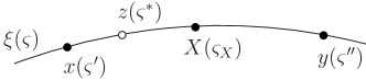
Figure 3: Arrangement of the points along the geodesic.

Let $\varsigma$ be the affine parameter of the geodesic connecting $x$ and $y$ (see Fig. 3) and $\xi(\varsigma)$ a function mapping $\varsigma$ onto the points of the geodesic, with

$$x^{\alpha}=\xi(\varsigma^{\prime}),\quad y^{\alpha}=\xi(\varsigma^{\prime\prime})\,.$$ (43)

The center coordinate lies in the middle of the geodesic, i.e. it corresponds to $\varsigma_{X}\equiv\frac{1}{2}(\varsigma^{\prime}+\varsigma^{\prime\prime})$. The relative coordinate is given by the sum of the infinitesimal distance vectors $d\xi^{\alpha}$ along the geodesic, all of which must have been submitted to parallel transfer to $\varsigma_{X}$ from the integration point on the curve. According to Winter (1985) this implies

$$X^{\alpha}\equiv X^{\alpha}_{xy}=\xi^{\alpha}\left(\varsigma_{X}\right),~{}s^{\alpha}\equiv s^{\alpha}_{xy}=(\varsigma^{\prime}-\varsigma^{\prime\prime})u^{\alpha}\left(\varsigma_{X}\right)\,.$$ (44)

All quantities in equations (41) are now recast in terms of $X^{\alpha}$ and $s^{\alpha}$. Up to higher order, proportional to the curvature tensor terms, the Laplace–Beltrami operator is given by Winter (1985)

$$\square_{x,y}\approx{\frac{1}{4}}D^{\alpha}D_{\alpha}+\frac{\partial^{2}}{\partial s^{\alpha}\partial s_{\alpha}}\pm D^{\alpha}\frac{\partial}{\partial s_{\alpha}}\,,$$ (45)

where $D_{\alpha}$ is the covariant derivative

$$D_{\alpha} \equiv\frac{\partial}{\partial X^{\alpha}}-\Gamma^{\beta}_{\alpha\gamma}s^{\gamma}\frac{\partial}{\partial s^{\beta}}\,.$$ (46)

Note that in (45) we have neglected the corrections proportional to the Riemann and Ricci tensors. Next, we Taylor expand the effective masses to first order around the center coordinate $X$

$$M^{2}\approx M^{2}(X)\pm{\textstyle\frac{1}{2}}s^{\alpha}D_{\alpha}M^{2}(X)\,,$$ (47)

where the minus sign corresponds to $y$ whereas the plus sign corresponds to $x$. The propagators on the left–hand side of (41) can also be reparameterized in terms of the center and relative coordinates: $G_{F}(x,y)\rightarrow\tilde{G}_{F}(X,s)$ and $G_{\rho}(x,y)\rightarrow\tilde{G}_{\rho}(X,s)$.

On the right–hand sides we have convolutions of functions of $x$ and $z$ and functions of $z$ and $y$. That is, we have to introduce the corresponding center and relative coordinates and perform the integration. Making use of the identity

$$(\varsigma^{\prime}+\varsigma^{*})=(\varsigma^{\prime}+\varsigma^{\prime\prime})+(\varsigma^{*}-\varsigma^{\prime\prime})=2\,\varsigma_{X}+(\varsigma^{*}-\varsigma^{\prime\prime})$$

and Taylor expanding around $\varsigma_{X}$, we obtain to first order

$$\Pi_{F}(x,z) \equiv\tilde{\Pi}_{F}(X_{xz},s_{xz})\approx\tilde{\Pi}_{F}(X,s_{xz})$$

$$+\left({\frac{\partial\tilde{\Pi}_{F}}{\partial\xi^{\alpha}}}\frac{d\xi^{\alpha}}{d\varsigma}+{\frac{\partial\tilde{\Pi}_{F}}{\partial u^{\alpha}}}\frac{du^{\alpha}}{d\varsigma}\right)\frac{\varsigma^{*}-\varsigma^{\prime\prime}}{2}\,.$$ (48)

Using furthermore the definition of the four–velocity and the geodesic equation

$$\frac{d\xi^{\alpha}}{d\varsigma}=u^{\alpha},\quad\frac{du^{\alpha}}{d\varsigma}=-\Gamma^{\alpha}_{\beta\gamma}u^{\beta}u^{\gamma}\,,$$ (49)

we can rewrite (V) in the form

$$\Pi_{F}(x,z)\approx\tilde{\Pi}_{F}(X,s_{xz})+{\textstyle\frac{1}{2}}s^{\alpha}_{zy}D_{\alpha}\tilde{\Pi}_{F}(X,s_{xz})\,,$$ (50)

where $s^{\alpha}_{zy}\equiv(\varsigma^{*}-\varsigma^{\prime\prime})u^{\alpha}(\varsigma_{X})$. Making use of the identity

$$(\varsigma^{\prime\prime}+\varsigma^{*})=(\varsigma^{\prime}+\varsigma^{\prime\prime})-(\varsigma^{\prime}-\varsigma^{*})=2\,\varsigma_{X}-(\varsigma^{\prime}-\varsigma^{*})$$

we get a similar expression for the functions of $z$ and $y$

$$G_{A}(z,y)\approx\tilde{G}_{A}(X,s_{zy})-{\textstyle\frac{1}{2}}s^{\alpha}_{xz}D_{\alpha}\tilde{G}_{A}(X,s_{zy})\,.$$ (51)

To perform the integration of the product of (50) and (51), we shift the coordinate origin to $\varsigma_{X}$ and replace the integration with respect to $z$ by integration with respect to distance $s_{Xz}$ from $X$ to $z$ along the geodesic. Moreover, we approximate $\sqrt{-g}_{z}$ by its value at the origin $\sqrt{-g}_{X}$.

The Kadanoff–Baym equations describe the dynamics of a system in terms of the spectral function and statistical propagator. The latter ones are functions of two coordinates in the four–dimensional space–time. By introducing center and relative coordinates we have traded one set of coordinates for another one. Performing the so–called Wigner transformation, one can also trade one of the arguments defined in the coordinate space for an argument defined in the momentum space. In curved space–time Winter (1985)

$$\tilde{G}_{F}(X,p) =\sqrt{-g}_{X}\int d^{4}s\,e^{ips}\tilde{G}_{F}(X,s)\,,$$ (52a)

$$\tilde{G}_{F}(X,s) =\frac{1}{\sqrt{-g}_{X}}\int\frac{d^{4}p}{(2\pi)^{4}}\,e^{-ips}\tilde{G}_{F}(X,p)\,.$$ (52b)

Note that in (52) and in the rest of the paper we use contravariant components of the space–time coordinates and covariant components of the momenta. Let us also note that

$$d\Pi^{4}_{p}\equiv\frac{1}{\sqrt{-g}_{X}}\frac{d^{4}p}{(2\pi)^{4}}$$

is the invariant volume element in momentum space. The definition of the Wigner transform of $\tilde{G}_{\rho}(X,s)$ differs from (52a) by a factor of $-i$ so that $\tilde{G}_{\rho}(X,p)$ is again real valued.

As follows from (52b), differentiation with respect to $s^{\alpha}$ is replaced after the Wigner transformation by $p^{\alpha}$

$$\frac{\partial}{\partial s^{\alpha}}\rightarrow-ip^{\alpha}\,.$$ (53)

Upon integration by parts we also see that $s^{\alpha}$ is replaced by differentiation with respect to $p^{\alpha}$:

$$s^{\alpha}\rightarrow-i\frac{\partial}{\partial p^{\alpha}}\,.$$ (54)

Consequently the Wigner transformed covariant derivative reads

$$D_{\alpha}\rightarrow{\cal D}_{\alpha}=\frac{\partial}{\partial X^{\alpha}}+\Gamma^{\beta}_{\alpha\gamma}p_{\beta}\frac{\partial}{\partial p_{\gamma}}\,.$$ (55)

Correlations between earlier and later times are exponentially suppressed, which leads to a gradual loss of the dependence on the initial conditions Berges and Borsanyi (2006a); Lindner and Muller (2006). Exploiting this fact, one can drop the $\theta$ function from the integrals in the difference equations (41). Furthermore we let the relative–time coordinate $s^{0}$ range from $-\infty$ to $\infty$ in order to perform the Wigner transformation, see Berges and Borsanyi (2006a, b) for a detailed discussion of these approximations. Then using (54) and (55) we obtain for the Wigner transform of the first term on the right–hand side of (41):

$${\textstyle\int} \sqrt{-g}_{z}d^{4}z~{}\Pi_{F}(x,z)G_{A}(z,y)\rightarrow$$

$$\tilde{\Pi}_{F}(X,p)\tilde{G}_{A}(X,p)+{\textstyle\frac{i}{2}}\{\tilde{\Pi}_{F}(X,p),\tilde{G}_{A}(X,p)\}_{PB}\,,$$ (56)

where the Poisson brackets are defined by

$$\{\tilde{A}(X,p),\tilde{B}(X,p)\}_{PB} \equiv\frac{\partial}{\partial p_{\alpha}}\tilde{A}(X,p){\cal D}_{\alpha}\tilde{B}(X,p)$$

$$-{\cal D}_{\alpha}\tilde{A}(X,p)\frac{\partial}{\partial p_{\alpha}}\tilde{B}(X,p)\,.$$ (57)

Comparing (V) to its Minkowski–space counterpart we see that the derivatives with respect to $X$ are replaced by the covariant derivatives, just as one would expect.

Wigner transforming the rest of the terms we obtain a rather lengthy expression which can be substantially simplified with the help of the relations between $\tilde{G}_{R}(X,p)$, $\tilde{G}_{A}(X,p)$, and $\tilde{G}_{\rho}(X,p)$. Recalling the Fourier transform of the $\theta$ function,

$${\textstyle\int}ds^{0}\exp(iws^{0})\theta(\pm s^{0})=\lim\limits_{\epsilon\rightarrow 0}\frac{\pm\,i}{\omega\pm i\epsilon},$$

we find that

$$\tilde{G}_{R}(X,p) =-\int\frac{d\omega}{2\pi}\frac{\tilde{G}_{\rho}(X,\vec{p},\omega)}{p_{0}-\omega+i\epsilon}\,,$$ (58a)

$$\tilde{G}_{A}(X,p) =-\int\frac{d\omega}{2\pi}\frac{\tilde{G}_{\rho}(X,\vec{p},\omega)}{p_{0}-\omega-i\epsilon}\,.$$ (58b)

From comparison of (58b) and (58a) it follows that

$$\tilde{G}_{A}(X,p)=\tilde{G}^{*}_{R}(X,p)\,.$$ (59)

Recalling furthermore that the $\delta$ function can be approximated by

$$\delta(\omega)=\lim\limits_{\epsilon\rightarrow+0}\frac{\epsilon}{\pi(\omega^{2}+\epsilon^{2})}\,,$$ (60)

we also find that

$$\tilde{G}_{R}(X,p)-\tilde{G}_{A}(X,p)=i\tilde{G}_{\rho}(X,p)\,.$$ (61)

Analogous relations also hold for the retarded and advanced components of the self–energy.

As can be inferred from (45) and (47), the Wigner transform of the left–hand side of (41) reads

$$\square_{x}-\square_{y}+M^{2}(x) -M^{2}(y)\rightarrow$$

$$-i\left(2p^{\alpha}{\cal D}_{\alpha}+D_{\alpha}M^{2}\frac{\partial}{\partial p_{\alpha}}\right)\,.$$ (62)

Introducing the quantity

$$\tilde{\Omega}(X,p)\equiv p^{\mu}p_{\mu}-M^{2}(X)-\tilde{\Pi}_{h}(X,p)\,,$$ (63)

where $\tilde{\Pi}_{h}(X,p)\equiv{\rm Re}\,\tilde{\Pi}_{R}(X,p)$, and collecting the terms on the right–hand side of the kinetic equation (41) one can write the kinetic equation for the Wigner transform of the statistical propagator in the compact form:

$$\{\tilde{\Omega}(X,p),\tilde{G}_{F} (X,p)\}_{PB}$$

$$=\tilde{G}_{F}(X,p)\tilde{\Pi}_{\rho}(X,p)-\tilde{\Pi}_{F}(X,p)\tilde{G}_{\rho}(X,p)$$

$$+\{\tilde{\Pi}_{F}(X,p),\tilde{G}_{h}(X,p)\}_{PB}\,,$$ (64)

where $\tilde{G}_{h}(X,p)\equiv{\rm Re}\,\tilde{G}_{R}(X,p)$. The same procedure leads also to a kinetic equation for the Wigner transform of the spectral function

$$\{\tilde{\Omega}(X,p),\tilde{G}_{\rho} (X,p)\}_{PB}$$

$$=\{\tilde{\Pi}_{\rho}(X,p),\tilde{G}_{h}(X,p)\}_{PB}\,.$$ (65)

As has been mentioned in the previous section, the exact quantum dynamical evolution of the system depends on its whole evolution history. Mathematically, this manifests itself in the memory integrals on the right–hand sides of (34). In fact, performing the linear order Taylor expansion around $X$, we take into account only a very short part of the history of the evolution. Since the expansion coefficients are defined at $X$, after the integration we obtain equations which are local in time.

Next we consider the Wigner transform of the constraint equation for the retarded propagator (V). On the left–hand side we have $\square_{x}+\square_{y}=2\partial_{s^{\alpha}}\partial_{s_{\alpha}}$, to first order in the covariant derivative, whereas $M^{2}(x)+M^{2}(y)\approx M^{2}(X)$. On the right–hand side the Poisson brackets cancel out and only the product of $\tilde{\Pi}_{R}(X,p)$ and $\tilde{G}_{R}(X,p)$ remains. Finally, the Wigner transform of the generalized $\delta$ function is just unity. Therefore, we get an algebraic equation for the Wigner transform of the retarded propagator

$$[\,p^{\mu}p_{\mu}-M^{2}(X)-\tilde{\Pi}_{R}(X,p)\,]\tilde{G}_{R}(X,p)=-1\,.$$ (66)

Equation (66) implies that the real part of the retarded propagator is given by

$$\tilde{G}_{h}(X,p)=\frac{-\tilde{\Omega}(X,p)}{\tilde{\Omega}^{2}(X,p)+{\textstyle\frac{1}{4}}\tilde{\Pi}^{2}_{\rho}(X,p)}\,.$$ (67)

Note that $\tilde{G}_{h}(X,p)$ vanishes on the mass shell, which is defined by the condition $\tilde{\Omega}(X,p)=0$. As follows from (59) and (61), the Wigner transform of the spectral function is twice the imaginary part of the retarded propagator:

$$\tilde{G}_{\rho}(X,p)=\frac{-\tilde{\Pi}_{\rho}(X,p)}{\tilde{\Omega}^{2}(X,p)+{\textstyle\frac{1}{4}}\tilde{\Pi}^{2}_{\rho}(X,p)}\,.$$ (68)

Equation (68) is also a solution of (V). To first order in the covariant derivative the Wigner–transform of the constraint equation for the statistical propagator reads

$$\tilde{\Omega}(X,p)\tilde{G}_{F}(X,p)={\textstyle\frac{1}{4}}\{\tilde{\Pi}_{F}(X,p),\tilde{G}_{\rho}(X,p)\}_{PB}$$

$$+{\textstyle\frac{1}{4}}\{\tilde{G}_{F}(X,p),\tilde{\Pi}_{\rho}(X,p)\}_{PB}+\tilde{\Pi}_{F}(X,p)\tilde{G}_{h}(X,p).$$ (69)

The constraint equation for $\tilde{G}_{F}(X,p)$ is no longer algebraic and can not be solved analytically in general. However, let us assume for a moment that the system is in thermal equilibrium. In this case all the quantities are constant in time and space and the Poisson brackets in (V) vanish identically. The solution of the resulting algebraic equation then reads

$$\tilde{G}^{eq}_{F}(p)=\frac{\tilde{\Pi}_{F}(p)}{\tilde{\Pi}_{\rho}(p)}\,\tilde{G}^{eq}_{\rho}(p)\,.$$ (70)

That is, we have obtained the fluctuation–dissipation relation. It only remains to calculate the ratio of the spectral and statistical self–energies. This can be done using the relation (30) and the KMS periodicity condition, $G(x,y)|_{x=0}=G(x,y)|_{x=-i\beta}$, where $\beta$ is the inverse temperature. Wigner–transforming this equation and using (70) we obtain

$$\tilde{G}^{(eq)}_{F}(p)=\left[n^{(eq)}(p)+{\textstyle\frac{1}{2}}\right]\tilde{G}^{(eq)}_{\rho}(p)\,,$$ (71)

where $n^{(eq)}$ is the Bose–Einstein distribution function.

To complete this section, we have to express the Wigner transforms of the spectral and statistical self–energies in terms of the Wigner transforms of the spectral function and statistical propagator. Using the definitions of the Wigner transformation and its inverse we find for the Wigner transform of a product of functions of the same arguments:

$$f_{1} (x,y)\ldots f_{n}(x,y)\rightarrow\widetilde{f_{1}\ldots f_{n}}(X,p)$$

$$\equiv{\textstyle\int}d\Pi^{4}_{p_{1}}\ldots d\Pi^{4}_{p_{n}}(2\pi)^{4}\sqrt{-g}_{X}\delta^{4}(-p+p_{1}+\ldots p_{n})$$

$$\hskip 99.58464pt\times\tilde{f}(X,p_{1})\ldots\tilde{f}(X,p_{n})\,.$$ (72)

Note that $\delta_{g}(q)\equiv\sqrt{-g}_{X}\,\delta(q)$ represents the momentum–space generalization of the $\delta$ function, invariant under coordinate transformations (this can be checked with help of the scaling property of the $\delta$ function). Keeping in mind that the definition of $\tilde{G}_{\rho}(X,p)$ contains an additional factor of $-i$ we can then write the Wigner transforms of (35) in the form

$$\tilde{\Pi}^{(3)}_{F}(X,p)= -\frac{\lambda^{2}}{6}[\,\widetilde{G^{3}_{F}}(X,p)+{\textstyle\frac{3}{4}}\widetilde{G_{F}G^{2}_{\rho}}(X,p)]\,,$$ (73a)

$$\tilde{\Pi}^{(3)}_{\rho}(X,p)= -\frac{\lambda^{2}}{6}[3\widetilde{G^{2}_{F}G_{\rho}}(X,p)+{\textstyle\frac{1}{4}}\widetilde{G^{3}_{\rho}}(X,p)]\,.$$ (73b)

The expression for the Wigner transform of the three–loop retarded self–energy can be obtained from (73) by replacing one of the $\tilde{G}_{\rho}$ by $\tilde{G}_{R}$. The Wigner transforms of the four–loop contributions (35) can be written in a similar way

$$\tilde{\Pi}^{(4)}_{F}(X,p)= \frac{\lambda^{3}}{2}[\widetilde{G_{F}G_{4F}}(X,p)+{\textstyle\frac{1}{4}}\widetilde{G_{\rho}G_{4\rho}}(X,p)]\,,$$ (74a)

$$\tilde{\Pi}^{(4)}_{\rho}(X,p)= \frac{\lambda^{3}}{2}[\widetilde{G_{F}G_{4\rho}}(X,p)+\widetilde{G_{\rho}G_{4F}}(X,p)]\,.$$ (74b)

Note, however, that $\tilde{G}_{4F}$ and $\tilde{G}_{4\rho}$ are Wigner transforms of convolutions of four two–point functions,

$$G_{4F}(x,y) ={\textstyle\int}\sqrt{-g}d^{4}z\,G_{F}(x,z)G_{R}(x,z)$$

$$\times[G^{2}_{F}(z,y)-{\textstyle\frac{1}{4}}G^{2}_{\rho}(z,y)]+\{x\leftrightarrow y\}\,,$$ (75a)

$$G_{4\rho}(x,y) ={\textstyle\int}\sqrt{-g}d^{4}z\,G_{F}(x,z)G_{R}(x,z)$$

$$\times[2G_{F}(z,y)G_{\rho}(z,y)]-\{x\leftrightarrow y\}\,,$$ (75b)

where we have used the definitions of the retarded and advanced propagators and dropped again the $\theta(z^{0})$ factor. Proceeding as in Eq. (V) and making use of the relations (59) and (61), we obtain for the Wigner transforms of $G_{4F}$ and $G_{4\rho}$

$$\tilde{G}_{4F}(X,p)=2[\widetilde{G^{2}_{F}}(X,p)+{\textstyle\frac{1}{4}}\widetilde{G^{2}_{\rho}}(X,p)]\widetilde{G_{F}\Re[G_{R}]}(X,p)$$

$$+{\textstyle\frac{1}{2}}\{\widetilde{G^{2}_{F}}(X,p)+{\textstyle\frac{1}{4}}\widetilde{G^{2}_{\rho}}(X,p),\widetilde{G_{F}G_{\rho}}(X,p)\}_{P.B.}\,,$$ (76a)

$$\tilde{G}_{4\rho}(X,p)=4\widetilde{G_{F}G_{\rho}}(X,p)\widetilde{G_{F}\Re[G_{R}]}(X,p)\,.$$ (76b)

Finally, the expression for the Wigner transform of the four–loop retarded self–energy can be obtained from (74b) by replacing $\tilde{G}_{\rho}$ with $\tilde{G}_{R}$ and $\tilde{G}_{4\rho}$ with $\tilde{G}_{4R}$. The latter one is related to $\tilde{G}_{4\rho}$ by Eq. (58a).

VI Boltzmann kinetics

The spectral function (68) has approximately Breit–Wigner shape with a width proportional to the spectral self–energy. The area under $G_{\rho}(X,p)$ is determined by the normalization condition,

$$\int\frac{g^{00}}{2\pi}\tilde{G}_{\rho}(X,p)\,p_{0}\,dp_{0}=1,$$ (77)

which is a direct consequence of (32) and the antisymmetry of the spectral function with respect to permutation of its arguments. In the limit of vanishing coupling constant the width of the spectral function approaches zero, whereas its on–shell value goes to infinity, see Eq. (68). Equation (60) then implies that in this limit the spectral function takes the quasiparticle form Kadanoff and Baym (1962)

$$\tilde{G}_{\rho}(X,p)=2\pi\,{\rm sign}(p_{0})\,\delta\left(g^{\mu\nu}p_{\mu}p_{\nu}-M^{2}\right)\,.$$ (78)

Note that (78) is consistent with the normalization condition (77). The signum–function appears in (78) because $\tilde{\Pi}_{\rho}(X,p)$ is an odd function of $p_{0}$. Since the magnitudes of $\tilde{\Pi}_{\rho}$, $\tilde{\Pi}_{h}$ and of the local term of the self–energy are controlled by the same coupling we have also neglected them in $\tilde{\Omega}(X,p)$. In the same limit Eq. (V) for the spectral function simplifies to

$$p^{\alpha}{\cal D}_{\alpha}\tilde{G}_{\rho}(X,p) =0$$ (79)

and indeed admits a quasiparticle solution (78). Note that Eqs. (79) and (78) state that the effective mass $M$ of the field quanta does not change as they move along the geodesic, just like it is the case for particles.

Motivated by the fluctuation–dissipation relation (71) we can trade the statistical propagator for some other function:

$$\tilde{G}_{F}(X,p)=\left[n(X,p)+{\textstyle\frac{1}{2}}\right]\tilde{G}_{\rho}(X,p)\,.$$ (80)

However, if both $\tilde{G}_{F}(X,p)$ and $\tilde{G}_{\rho}(X,p)$ are smooth functions then relation (80) is merely a definition of $n(X,p)$. In the quasiparticle approximation the spectral function is divergent and forces the momentum argument of $n$ to be on the mass shell. For this reason the quasiparticle approximation for the statistical propagator (80) is usually referred to as the Kadanoff–Baym Ansatz Kadanoff and Baym (1962); Berges (2004).

Let us now tentatively put the coupling constant to zero. In this case the right–hand sides of the kinetic equations (V) and (V) vanish. In this case $\tilde{G}_{F}(X,p)$ and $\tilde{G}_{\rho}(X,p)$ are constant in space and time even if the system is out of equilibrium. If we now “increase” the coupling constant again, then the gain and loss terms on the right–hand side of (V) will induce nontrivial dynamics for the statistical propagator. This in turn will induce a time and space dependence of the spectral and statistical propagators thus leading to nonvanishing Poisson brackets on the right–hand sides of the kinetic equations. The magnitude of the derivatives with respect to the time and space coordinates are therefore proportional to some (positive) power of the coupling constant. Consequently the contribution of the Poisson brackets in (V) is effectively of higher order in $\lambda$ than the contribution of the gain and loss terms. These considerations justify the dropping of the Poisson brackets and of the local and nonlocal contributions to the effective field mass in the kinetic equations. In other words, they legitimate the use of the quasiparticle approximation.

As has been argued above, the Poisson brackets partially take into account the memory effects. Neglecting the Poisson brackets we completely ignore the previous evolution of the system. Physically this corresponds to the Stosszahlansatz of Boltzmann.

From Eqs. (V), (79) and (80) it follows that in this approximation the kinetic equation for the statistical propagator turns into an equation for the evolution of the one–particle distribution function $n(X,p)$:

$$[\,p^{\alpha} {\cal D}_{\alpha}n(X,p)]\tilde{G}_{\rho}(X,p)$$

$$={\textstyle\frac{1}{2}}[\tilde{\Pi}_{>}(X,p)\tilde{G}_{<}(X,p)-\tilde{G}_{>}(X,p)\tilde{\Pi}_{<}(X,p)]\,,$$ (81)

where we have introduced

$$\tilde{G}_{\gtrless}(X,p)\equiv\tilde{G}_{F}(X,p)\pm{\textstyle\frac{1}{2}}\tilde{G}_{\rho}(X,p)\,$$ (82)

and their self–energy analogs $\tilde{\Pi}_{\gtrless}(X,p)$. The symmetry (antisymmetry) of the statistical (spectral) propagator with respect to permutation of its arguments and the definition of the Wigner transformation imply that

$$\tilde{G}_{F}(X,p)=\tilde{G}_{F}(X,-p),\,\tilde{G}_{\rho}(X,p)=-\tilde{G}_{\rho}(X,-p)\,.$$ (83)

Therefore, for a single real scalar field, we have

$$\tilde{G}_{\gtrless}(X,-p)=\tilde{G}_{\lessgtr}(X,p)\,,$$ (84)

and a similar relation for the self–energies.

Explicit expressions for $\tilde{\Pi}_{\gtrless}(X,p)$ can be obtained after some algebra from Eqs. (73) and (74). For illustration purposes we first derive $\Pi_{\gtrless}(x,y)$ and then perform the Wigner transformation. Using the decomposition

$$G(x,y)=\theta(x^{0}-y^{0})G_{>}(x,y)+\theta(y^{0}-x^{0})G_{<}(x,y)$$ (85)

we obtain for the three–loop contribution

$$\Pi^{(3)}_{\gtrless}(x,y)=-\frac{\lambda^{2}}{6}G_{\gtrless}(x,y)G_{\gtrless}(x,y)G_{\gtrless}(x,y)\,.$$ (86)

Its Wigner transform reads

$$\tilde{\Pi}^{(3)}_{\gtrless}(X,p)= -\frac{\lambda^{2}}{6}{\textstyle\int}d\Pi^{4}_{k}d\Pi^{4}_{q}d\Pi^{4}_{t}(2\pi)^{4}\delta_{g}(-p-t+k+q)$$

$$\times\tilde{G}_{\lessgtr}(X,t)\tilde{G}_{\gtrless}(X,k)\tilde{G}_{\gtrless}(X,q)$$ (87)

where we have used relation (84). It describes $2\leftrightarrow 2$ scattering and corresponds to the tree–level Feynman diagram in Fig. 4.

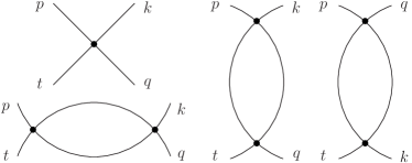
Figure 4: Feynman diagrams of $2\leftrightarrow 2$ scattering at tree and one–loop levels.

Expression for the four–loop contribution contains integration over the contour

$$\tilde{\Pi}^{(4)}_{\gtrless}(x,y)=\frac{\lambda^{3}}{2}G_{\gtrless}(x,y){\textstyle\int}\sqrt{-g}_{z}d^{4}z\,\theta(z^{0})\times$$ (88)

$$[G_{F}(x,z)G_{R}(x,z)G^{2}_{\gtrless}(z,y)+G^{2}_{\gtrless}(x,z)G_{A}(z,y)G_{F}(z,y)].$$

After some algebra we obtain for the Wigner transform of (88) in the Boltzmann approximation (that is, with the Poisson brackets neglected)

$$\tilde{\Pi}^{(4)}_{\gtrless}( X,p)=\frac{\lambda^{3}}{2}{\textstyle\int}d\Pi^{4}_{k}d\Pi^{4}_{q}d\Pi^{4}_{t}(2\pi)^{4}\delta_{g}(-p-t+k+q)$$

$$\times\tilde{G}_{\lessgtr}(X,t)\tilde{G}_{\gtrless}(X,k)\tilde{G}_{\gtrless}(X,q)\,L(X,k+q)\,,$$ (89)

where

$$L(X,p)\equiv{\textstyle\int}d \Pi^{4}_{k}d\Pi^{4}_{q}(2\pi)^{4}\delta_{g}(-p+k+q)$$

$$\times 2\,\tilde{G}_{F}(X,k)\tilde{G}_{h}(X,q)\,.$$ (90)

From (VI) it follows that $L(X,p)$ is the same for the forward and inverse processes. As is demonstrated in Appendix A it corresponds to the integrals of the one–loop Feynman diagrams in Fig. 4.

Let us note here that the contribution(s) of a particular term of the 2PI effective action to the Boltzmann equation can be deduced by cutting the 2PI diagrams by a connected line in all possible ways. The three–loop contribution, for instance, can be cut in only one way and the result can be represented as a product of two tree–level scattering diagrams. The four–loop contribution can be cut in three equivalent ways and the result can be represented as a product of tree–level and one–loop scattering diagrams, see Fig. 5.

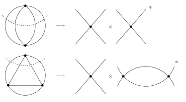
Figure 5: The correspondence between the diagrams contributing to the 2PI effective action and the contributions to the Boltzmann collision terms.

There are two five–loop loop contributions to the effective action Berges (2004). Applying the same procedure to one of them we would obtain interference terms of two one–loop scattering diagrams and interference of tree–level and two–loop scattering diagrams. Cutting the second, “eye”, diagram we would obtain interference of tree–level and two–loop scattering diagrams and also interference of two $2\rightarrow 4$ diagrams.

The quasiparticle approximation (78) for $\tilde{G}_{F}(X,k)$ in (VI) forces one of the intermediate states in the loop to be on the mass shell. On the contrary $\tilde{G}_{h}$, which describes the second intermediate state in the loop, vanishes on the mass shell. That is, the real intermediate state contributions ($2\rightarrow 2$ scattering into two on–shell states followed by another $2\rightarrow 2$ scattering) are automatically subtracted from the four–loop self–energies.

Also note, that initial and final states and on–shell intermediate states can be clearly distinguished in this formalism: the former ones are described by $\tilde{G}_{\gtrless}$ components, whereas the latter ones by $\tilde{G}_{F}$ or $\tilde{G}_{\rho}$ components. Performing the integration and taking into account that one of the intermediate states is on–shell, we obtain the following expression for the loop integral:

$$L(X,p) =\lim\limits_{\epsilon\rightarrow 0}{\textstyle\int}\frac{d{\bf k}}{(2\pi)^{3}}\frac{2n(X,{\bf k})+1}{2E_{k}}$$

$$\times \left[\frac{p^{2}-2pk}{(p^{2}-2pk)^{2}+\epsilon^{2}}+\frac{p^{2}+2pk}{(p^{2}+2pk)^{2}+\epsilon^{2}}\right]\,,$$ (91)

where $k=(E_{k},{\bf k})$ is the on–shell four–momentum expressed in terms of the “physical” components: $E_{k}\equiv k_{0}/\sqrt{g_{00}}$, etc. In (VI) the background plasma “affects” only one of the internal lines; the other one is off–shell and we can not associate the particle number density with it.

Next, we integrate the left– and right–hand side of (VI) over $p_{0}$ and choose the positive energy solution of (78) on the left–hand side. On the right–hand side both, the positive and the negative energy, solutions contribute. For positive $p_{0}$ momentum–energy conservation allows the following three combinations:

$$a)\quad k_{0}>0,\quad q_{0}>0,\quad t_{0}>0\,,$$

$$b)\quad k_{0}>0,\quad q_{0}<0,\quad t_{0}<0\,,$$

$$c)\quad k_{0}<0,\quad q_{0}>0,\quad t_{0}<0\,.$$

As far as the three–loop self–energy (VI) is concerned, each combination leads to the same result, i.e. an overall factor of $3$ appears. For the four–loop self–energy the arising terms are not equal due to the presence of the loop integral $L$ in (VI). Taking this into account and comparing (VI) and (VI) we see that in the 2PI formalism the effective coupling at nonzero particle number density at one–loop level contains a sum of three $L(X,p)$ functions with the arguments corresponding to $s$–, $t$– and $u$–channel scattering:

$$\varLambda^{2}(X,k,q,t) \equiv\lambda^{2}(1-\lambda[L(X,k+q)$$

$$+L(X,k-t)+L(X,q-t)])\,.$$ (92)

After some algebra, the use of (84) and redefinition of the momenta we finally arrive at the Boltzmann equation for the distribution function:

$$p^{\alpha}{\cal D}_{\alpha}n(X,{\bf p})= -\frac{\pi}{16}\int\frac{d{\bf k}}{(2\pi)^{3}}\frac{d{\bf q}}{(2\pi)^{3}}\frac{d{\bf t}}{E_{k}E_{q}E_{t}}\,\delta(E_{p}+E_{t}-E_{q}-E_{k})\delta({\bf p}+{\bf t}-{\bf q}-{\bf k}\,)\,\varLambda^{2}(X,{\bf k},{\bf q},{\bf t})$$

$$\times\left\{n(X,{\bf p})n(X,{\bf t})[n(X,{\bf k})+1][n(X,{\bf q})+1]-[n(X,{\bf p})+1][n(X,{\bf t})+1]n(X,{\bf k})n(X,{\bf q})\right\}\,.$$ (93)

It is interesting, that the only remnant of the curved structure of space–time is the covariant derivative on the left–hand side of the Boltzmann equation. In the case of greatest practical interest – the Friedmann–Robertson–Walker universe – it takes the form

$$p^{\alpha}{\cal D}_{\alpha}n=\frac{E}{a}\left(\frac{\partial}{\partial\eta}-\frac{{\bf p}^{2}}{E}{\cal H}\frac{\partial}{\partial E}\right)n\,,\quad{\cal H}\equiv\frac{a^{\prime}}{a}\,,$$ (94)

where $\eta$ is the conformal time. An integral form of the Boltzmann equation in the FRW universe as well as in a space–time with linearly perturbed FRW metric can be found, for instance, in Kartavtsev and Besak (2008).

On the right–hand side, all the $\sqrt{-g}_{X}$ factors have disappeared due to the introduction of the “physical” momenta and energies. In other words, the transition amplitudes in the scattering terms are independent of the space–time metric, which justifies many earlier calculations. It is also remarkable that if only pointlike interactions (i.e. only the three–loop contribution to the 2PI effective action in the considered case) are taken into account, Eq. (VI) coincides with the classical Boltzmann equation with the collision term calculated in vacuum. The inclusion of four– (and higher–loop) corrections to the effective potential induces further terms in the Boltzmann equation. These terms correspond to the remnant space–time integrals in the self–energy and involve additional momentum integrals over the distribution functions.

VII Summary and conclusions

In this paper we have considered the dynamics of an out–of–equilibrium quantum system in a background gravitational field in the Schwinger–Keldysh formalism . As one would expect, the resulting equations turned out to be covariant generalizations of their Minkowski–space counterparts.

Remarkably, in the Boltzmann approximation the only remnant of the curved structure of the space–time is the covariant derivative on its left–hand side. The matrix elements of the scattering terms on the right–hand side are independent of the metric. This justifies earlier calculations where this has been assumed implicitly. Furthermore, if only the tree–level processes are taken into account, then the resulting equation coincides with the Boltzmann equation with the collision term calculated in vacuum. Processes described by loop diagrams, which induce corrections to the self–coupling, involve additional momentum integrals over the distribution functions, so that the resulting contributions differ from those calculated in vacuum.

Interestingly, loop corrections, i.e. processes with intermediate off–shell states, can be taken into account even if the quasiparticle Ansatz is applied. As far as on–shell intermediate states are concerned, there is a clear distinction between them and the initial and final states: the former ones are described by $\tilde{G}_{F}$ (or $\tilde{G}_{\rho}$) components, whereas the latter ones are given by $\tilde{G}_{\gtrless}$ components, see Eqs. (VI) and (VI). It is important that in the used formalism the problem of double–counting, which is cured by a real intermediate state subtraction procedure in the standard approach, does not arise at all.

For leptogenesis, this implies that whereas the washout processes described by contact interactions (they are present for instance in the supersymmetric extensions of the Standard Model) can be treated essentially classically, the correct treatment of the decay processes (which generate the asymmetry) and the scattering processes mediated by the right–handed neutrino (which washout the asymmetry) requires the use of the Kadanoff–Baym approach.

Since the peculiarities of the calculation, related to the presence of a background gravitational field, are determined only by transformation properties of the fields – scalar fields in the present case – the developed formalism can be applied to arbitrary systems of scalar fields without any modifications. In Garny et al. (2009b) we study further implications of this formalism for leptogenesis and calculate the vertex contribution to the CP–violating parameter at nonzero particle densities in the framework of a toy model that qualitatively reproduces the features of popular leptogenesis models. The analysis of the self–energy contributions to the CP–violating parameter will be performed in Garny et al. (2009c).

Acknowledgements

AH was supported by the “Sonderforschungsbereich” TR27. We thank Markus Michael Müller and Mathias Garny for sharing their insights in nonequilibrium quantum field theory and for very helpful discussions.

Appendix A $2\leftrightarrow 2$ scattering

The tree–level amplitude of $2\leftrightarrow 2$ scattering (see Fig. 4) in Minkowski space–time is given by

$$M^{tree}_{fi}=-i\lambda\,.$$ (95)

There are also three one–loop diagrams which contribute to the scattering amplitude. Their contribution reads

$$M^{loop}_{fi}=\frac{-\lambda^{2}}{2(2\pi)^{4}}\int\frac{d^{4}\xi\,d^{4}\eta\,\delta(-\sigma+\xi+\eta)}{[\xi^{2}-M^{2}+i\epsilon][\eta^{2}-M^{2}+i\epsilon]}\,,$$ (96)

where $\sigma$ is equal to $k+q$, to $k-t$ or $q-t$ (see Fig. 4). Because of the presence of the $\delta$–function one of the integrations (for instance, over $\eta$) can be performed trivially. Calculating residues of the integrand we can perform the integration over $d\xi_{0}$. The result of the integration reads

$$M^{loop}_{fi}=\frac{i\lambda^{2}}{2(2\pi)^{3}}\int\frac{d\xi^{3}}{2E_{\xi}}\left[\frac{1}{\xi^{2}+2\xi\sigma}+\frac{1}{\xi^{2}-2\xi\sigma}\right]\,.$$ (97)

The quantity which enters the right–hand side of the Boltzmann equation is the amplitude modulo squared. To leading order in small $\lambda$ it is given by

$$|M_{fi}|^{2}=\lambda^{2}(1- \lambda[L^{vac}(k+q)$$

$$+L^{vac}(k-t)+L^{vac}(q-t)])\,,$$ (98)

where $L^{vac}(\sigma)$ coincides with (VI) if $n(X,{\bf k})$ and $\epsilon$ are set to zero. The former condition arises from the fact that in this Appendix we calculate the scattering amplitudes in vacuum, whereas the latter one is related to the fact that we have not subtracted the contributions of real intermediate states to the one–loop amplitude. Comparing (A) with (VI) we conclude that $L(X,p)$ indeed describes the integrals of the one–loop diagrams.

References

- Sakharov (1967) A. D. Sakharov, JETP Letters 5, 24 (1967).
- Bernstein (1988) J. Bernstein, Kinetic Theory in the Expanding Universe (Cambridge University Press, Cambridge, 1988).
- de Groot et al. (1980) S. R. de Groot, W. A. van Leeuwen, and C. G. van Weert, Relativistic Kinetic Theory (North-Holland Publ. Comp., Amsterdam, 1980).
- Cercignani and Kremer (2002) C. Cercignani and G. M. Kremer, The Relativistic Boltzmann Equation: Theory and Applications (Birkhaeuser, Basel, Boston, 2002).
- Liboff (2003) R. L. Liboff, Kinetic Theory (Springer, New York, 2003), 3rd ed.
- Kadanoff and Baym (1962) L. Kadanoff and G. Baym, “Quantum Statistical Mechanics” (Benjamin, New York, 1962).
- Berges (2002) J. Berges, Nucl. Phys. A699, 847 (2002), eprint hep-ph/0105311.
- Aarts and Berges (2001) G. Aarts and J. Berges, Phys. Rev. D64, 105010 (2001), eprint hep-ph/0103049.
- Lindner and Muller (2006) M. Lindner and M. M. Muller, Phys. Rev. D73, 125002 (2006), eprint hep-ph/0512147.
- Lindner and Muller (2008) M. Lindner and M. M. Muller, Phys. Rev. D77, 025027 (2008), eprint 0710.2917.
- Berges et al. (2005a) J. Berges, S. Borsanyi, and C. Wetterich, Nucl. Phys. B727, 244 (2005a), eprint hep-ph/0505182.
- Juchem et al. (2004) S. Juchem, W. Cassing, and C. Greiner, Nucl. Phys. A743, 92 (2004), eprint nucl-th/0401046.
- Fukugita and Yanagida (1986) M. Fukugita and T. Yanagida, Phys. Lett. B174, 45 (1986).
- Buchmuller and Fredenhagen (2000) W. Buchmuller and S. Fredenhagen, Phys. Lett. B483, 217 (2000), eprint hep-ph/0004145.
- De Simone and Riotto (2007) A. De Simone and A. Riotto, JCAP 0708, 002 (2007), eprint hep-ph/0703175.
- Calzetta and Hu (1987) E. Calzetta and B. L. Hu, Phys. Rev. D35, 495 (1987).
- Calzetta et al. (1988) E. Calzetta, S. Habib, and B. L. Hu, Phys. Rev. D37, 2901 (1988).
- Ramsey and Hu (1997) S. A. Ramsey and B. L. Hu, Phys. Rev. D56, 661 (1997), eprint gr-qc/9706001.
- Tranberg (2008) A. Tranberg (2008), eprint arXiv:0806.3158.
- Pilaftsis and Underwood (2004) A. Pilaftsis and T. E. J. Underwood, Nucl. Phys. B692, 303 (2004), eprint hep-ph/0309342.
- Pilaftsis and Underwood (2005) A. Pilaftsis and T. E. J. Underwood, Phys. Rev. D72, 113001 (2005), eprint hep-ph/0506107.
- Garny et al. (2009a) M. Garny, A. Hohenegger, A. Kartavtsev, and M. Lindner (2009a), in preparation.
- Basler (1993) M. Basler, Fortschr. Phys. 41, 1 (1993).
- Toms (1987) D. J. Toms, Phys. Rev. D 35, 3796 (1987).
- Schwinger (1961) J. S. Schwinger, J. Math. Phys. 2, 407 (1961).
- Keldysh (1965) L. V. Keldysh, Sov. Phys. JETP 20, 1018 (1965).
- Chou et al. (1985) K.-c. Chou, Z.-b. Su, B.-l. Hao, and L. Yu, Phys. Rept. 118, 1 (1985).
- Danielewicz (1984) P. Danielewicz, Annals Phys. 152, 239 (1984).
- Zaidi (1983) M. h. Zaidi, Fortsch. Phys. 31, 403 (1983).
- Cornwall et al. (1974) J. M. Cornwall, R. Jackiw, and E. Tomboulis, Phys. Rev. D 10, 2428 (1974).
- Berges (2004) J. Berges, AIP Conf. Proc. 739, 3 (2004), eprint hep-ph/0409233.
- Isham (1978) C. J. Isham, Proceedings of the Royal Society of London. Series A, Mathematical and Physical Sciences 362, 383 (1978), ISSN 00804630.
- Landau and Lifshitz (1981) L. D. Landau and E. M. Lifshitz, “Course of Theoretical Physics 2: The Field Theory” (Pergamon Press, Oxford, 1981).
- Berges and Borsanyi (2006a) J. Berges and S. Borsanyi, Eur. Phys. J. A29, 95 (2006a), eprint hep-th/0512010.
- van Hees and Knoll (2001) H. van Hees and J. Knoll, Phys. Rev. D65, 025010 (2001), eprint hep-ph/0107200.
- Blaizot et al. (2003) J.-P. Blaizot, E. Iancu, and U. Reinosa, Phys. Lett. B568, 160 (2003), eprint hep-ph/0301201.
- Berges et al. (2005b) J. Berges, S. Borsanyi, U. Reinosa, and J. Serreau, Annals Phys. 320, 344 (2005b), eprint hep-ph/0503240.
- Arrizabalaga et al. (2005) A. Arrizabalaga, J. Smit, and A. Tranberg, Phys. Rev. D72, 025014 (2005), eprint hep-ph/0503287.
- Borsanyi and Reinosa (2008) S. Borsanyi and U. Reinosa (2008), eprint 0809.0496.
- Garny and Muller (2009) M. Garny and M. M. Muller (2009), eprint 0904.3600.
- Bernstein (1987) J. Bernstein, The Physics of Phase Space (Springer–Verlag, Berlin, 1987).
- Winter (1985) J. Winter, Phys. Rev. D 32, 1871 (1985).
- Berges and Borsanyi (2006b) J. Berges and S. Borsanyi, Phys. Rev. D74, 045022 (2006b), eprint hep-ph/0512155.
- Špička and Lipavský (1995) V. Špička and P. Lipavský, Phys. Rev. B 52, 14615 (1995).
- Köhler (1992) H. S. Köhler, Phys. Rev. C 46, 1687 (1992).
- Köhler and Malfliet (1993) H. S. Köhler and R. Malfliet, Phys. Rev. C 48, 1034 (1993).
- Köhler and Morawetz (2001) H. S. Köhler and K. Morawetz, Phys. Rev. C 64, 024613 (2001).
- Morozov and Röpke (2006a) V. G. Morozov and G. Röpke, Cond. mat. Phys. 9, 473 (2006a).
- Morozov and Röpke (2006b) V. G. Morozov and G. Röpke, Journal of Physics 35, 110 (2006b).
- Kartavtsev and Besak (2008) A. Kartavtsev and D. Besak, Phys. Rev. D78, 083001 (2008), eprint 0803.2729.
- Garny et al. (2009b) M. Garny, A. Hohenegger, A. Kartavtsev, and M. Lindner (2009b), eprint ArXiV: 0909.1559.
- Garny et al. (2009c) M. Garny, A. Hohenegger, A. Kartavtsev, and M. Lindner (2009c), in preparation.