Radiative Hydrodynamical Studies of Irradiated Atmospheres

Abstract

Transiting planets provide a unique opportunity to study the atmospheres of extra-solar planets. Radiative hydrodynamical models of the atmosphere provide a crucial link between the physical characteristics of the atmosphere and the observed properties. Here I present results from 3D simulations which solve the full Navier-Stokes equations coupled to a flux-limited diffusion treatment of radiation transfer for planets with 1, 3, and 7 day periods. Variations in opacity amongst models leads to a variation in the temperature differential across the planet, while atmospheric dynamics becomes much more variable at longer orbital periods. I also present 3D radiative simulations illustrating the importance of distinguishing between optical and infrared opacities.

1 Introduction

The abundance of close-in planets coupled with the wealth of information that can be deduced from the fraction that transit their host stars is now allowing us to probe our understanding of the physics of atmospheres through radiative hydrodynamical modelling. A number of approaches to this problem exist within the community. The physics of radiation and hydrodynamics are both extremely important, and there are several approaches currently utilized. Below I separate the approaches to both the dynamical and radiation aspects. Although this is not an exhaustive list, I believe it encapsulates the most widely utilized approaches in the field.

Dynamical Methods
Equivalent Barotropic Equations (2D)
Shallow Water Equations (3D)
Full Navier-Stokes Equations (3D)
Radiative Transfer Methods
Relaxation Methods
Flux-limited Radiative Diffusion
Coupled Radiation/Thermal Energy Equations
Full Wavelength Dependent Radiative Transfer

Ideally, we would solve the full 3D Navier-Stokes coupled with wavelength dependent radiative transfer. However, such a task is well beyond our computational resources, so groups working in this area select a method from one or both lists with which to tackle the problem. Although selecting methods with many built-in assumptions allows for high resolution studies, one runs the risk of missing fundamental physics crucial for a full understanding of the atmospheres. On the flip side, as with all numerical studies, the more exact your method, the more difficult and longer it takes to simulate. For a comparison of methods please see [Dobbs-Dixon et al. (2008), Dobbs-Dixon & Lin (2008)] or [Showman et al (2008), Showman et al (2008)].

In the following proceedings I will describe results from simulations utilizing the full 3D Navier-Stokes equations (described in Section (2)). In Section (3), I couple these with the flux-limited radiative transfer in simulations which solve a single equation for the energy of the radiation and gas components. These simulations exhibit a range of behavior for different opacities and orbital periods. I show that the local value of opacity is crucial in determining the efficiency of heat re-distribution to the night-side. In Section (4) I present results of simulations again solving the full Navier-Stokes equations, but now solving separate energy equations for the radiation and gas components. Decoupling these equations allows for the introduction of multiple opacities corresponding to both incident stellar and local radiation. As I show, this distinction is crucial in reproducing the observed upper atmosphere temperature inversions. I conclude in Section (5) with a discussion of the results.

2 Navier-Stokes Equations

Planetary atmospheres are simulated using a three-dimensional radiative hydrodynamical model in spherical coordinates $\left(r,\phi,\theta\right)$. The equations of continuity and momentum are given by

$${{\partial\rho}\over{\partial t}}+\nabla\cdot\left(\rho{\bf u}\right)=0$$ (1)

and

$${{\partial{\bf u}}\over{\partial t}}+\left({\bf u}\cdot\nabla\right){\bf u}=-\frac{1}{\rho}\nabla{P}+\frac{1}{\rho}\nabla{\Phi}-2{\bf\Omega\times u}-{\bf\Omega\times}\left({\bf\Omega\times r}\right)$$ (2)

where $\Omega$ is the rotation frequency and the $\Phi=-{GM_{p}\over r}$ is the gravitational potential.

As mentioned above, I present two separate sets of simulations in this proceeding. For those presented in Section (3), the radiative and thermal portions are combined into a single equation. The energy equation can then be written as

$$\left[{{\partial\epsilon}\over{\partial t}}+({\bf u}\cdot\nabla)\epsilon\right]=-P\,\nabla\cdot{\bf u}-\nabla\cdot{\bf F}$$ (3)

where $\epsilon=c_{v}\rho T$ is the internal energy density, $T$ is the local gas temperature, $c_{v}$ is the specific heat, and ${\bf F}$ is the radiative flux. The numerical techniques utilized in solving Equations (1)-(3) are described in [Dobbs-Dixon et al. (2008), Dobbs-Dixon & Lin (2008)].

The final ingredient for solving the energy balance in the atmosphere is a closure relation linking the flux ${\bf F}$ back to the radiation energy density. Here we utilize the flux-limited diffusion (FLD) approximation of [Levermore & Pomraning (1981), Levermore & Pomraning (1981)], where

$${\bf F}=-\lambda{\frac{c}{\rho\kappa_{R}\left(T,P\right)}}\nabla E_{R}.$$ (4)

In the above $E_{R}=aT^{4}$ and $\lambda$ is a spatial and temporally variable flux-limiter providing the closure relationship between flux and radiation energy density. The functional form of $\lambda$ is given by

$$\lambda=\frac{2+R}{6+3R+R^{2}},$$ (5)

where

$$R=\frac{1}{\rho\kappa_{R}\left(T,P\right)}\frac{|\nabla E_{R}|}{E_{R}}.$$ (6)

FLD allows for the simultaneous study of optically thin and optically thick gas, correctly reproducing the limiting behavior of the radiation at both extremes. In the optically thick limit the flux becomes the standard

$${\bf F}=-\frac{4acT^{3}}{3\rho\kappa_{R}\left(T,P\right)}\nabla T.$$ (7)

For the optically thin streaming limit, Equation (4) becomes $|{\bf F}|=cE_{R}$. Between these limits Equation (5) is chosen to approximate the full radiative transfer models of [Levermore & Pomraning (1981), Levermore & Pomraning (1981)].

3 Orbital Period and Opacity Variations

In this section I present simulations solving Equations (1)-(3) in a planet similar to HD 209458b, but for a variety of opacities and orbital periods. Opacity is a crucial factor in determining the efficiency of energy transport through the atmosphere. Therefore, I present separate results utilizing both the higher interstellar opacities ([Pollack et al. (1985), Pollack et al. (1985)] for lower temperatures coupled with [Alexander & Ferguson (1994), Alexander & Ferguson (1994)] for higher temperatures) and also lower line opacities of [Freedman et al. (2008), Freedman et al. (2008)]. Both sets of opacities are temperature and pressure dependent. Although it is now thought that the opacities of [Freedman et al. (2008), Freedman et al. (2008)] more closely represent the actual planetary opacities, it is clear that there is great diversity among the observed properties. Opacity may likely be a major factor in this diversity, so understanding how the dynamics and energy transfer change with varying opacity is quite important.

In Figure (1) I show the effect of opacity on the temperature at the photosphere of a synchronously rotating planet at an orbital distance of $0.04$ AU. As is clear from Figure (1), the higher the opacity the lower the night-side temperature. Night-side temperatures in a planet with high interstellar opacities are around $300$ K, while the night-side of a planet with lower opacity is around $700$ K. This difference can be easily understood by considering that the depth at which radiation is deposited changes with opacity. For large opacities the stellar energy is deposited high in the atmosphere where cooling timescales are relatively short. The flow is not able to effectively advect energy around the planet before it cools. For the lower opacity model, the stellar energy is deposited deeper in the atmosphere where cooling timescales become comparable to the crossing timescale. The efficiency of energy advection is also evident in the lobes that extend onto the night-side at both the equator (in the eastward direction) and the poles (in the westward direction). These regions correspond to the largest eastward and westward flow velocities respectively, thus the shortest crossing timescales. In general the night-side temperature can be calculated by equating the crossing and radiative timescales ([Burkert et al. (2005), Burkert et al. (2005)]). This gives a opacity dependent temperature that can be expressed as

$$T_{n}=\left(\frac{4vc_{s}^{2}}{3\pi\kappa_{d}\sigma R_{p}}\right)^{1/4}.$$ (8)

This is explored in greater detail in [Dobbs-Dixon et al. (2008), Dobbs-Dixon & Lin (2008)].

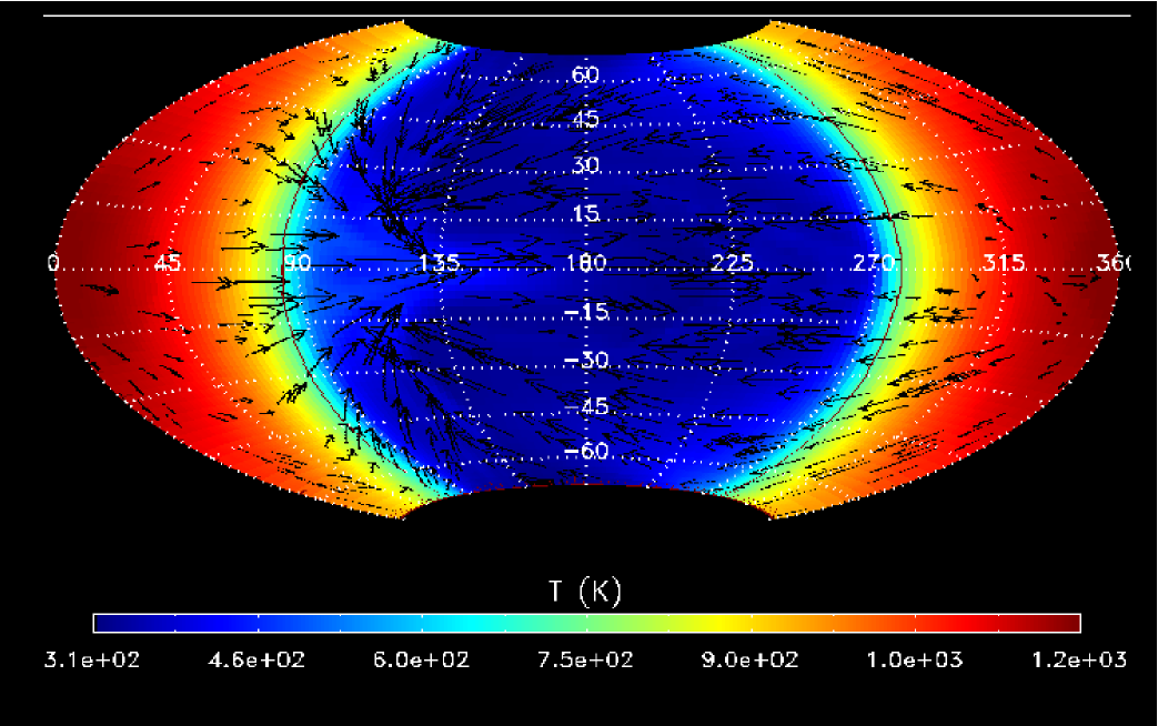
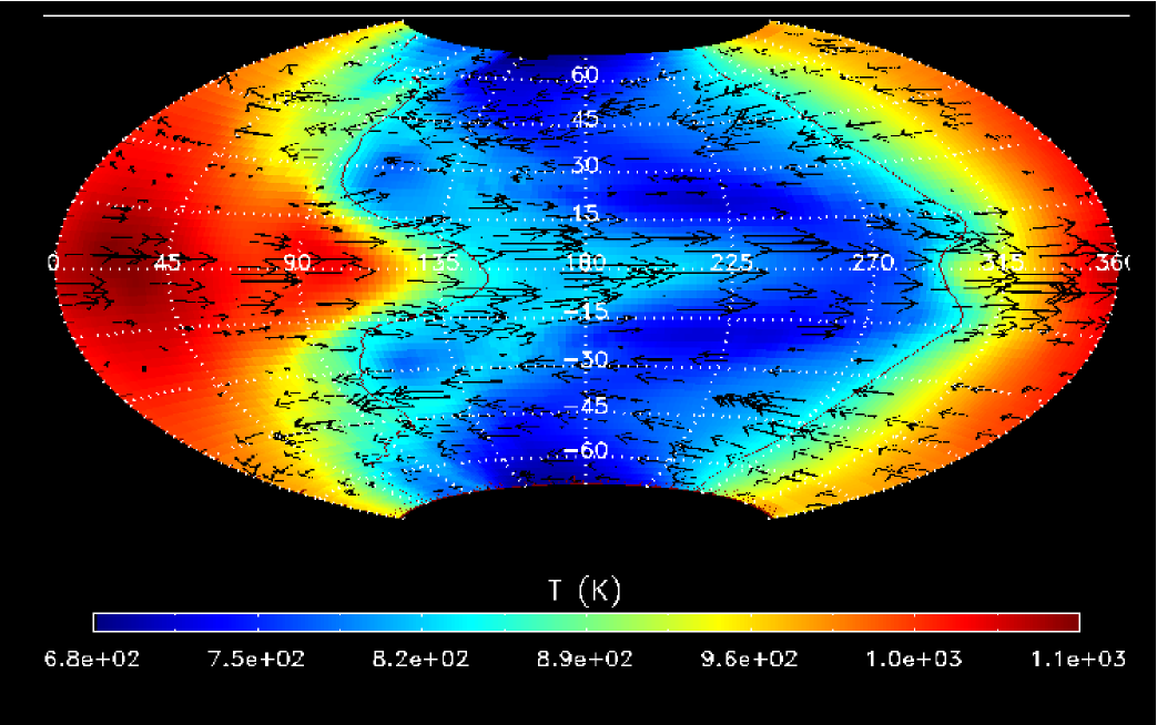
Figure 1: Temperature variations at the photosphere of irradiated planets synchronously rotating at orbital periods of 3-days. The left panel shows results using large interstellar opacities, while the right panel shows results using lower [Freedman et al. (2008), Freedman et al. (2008)] opacities. The subsolar point is located at zero degrees. Photospheric velocities are shown with the over-plotted arrows.

Given the rapidly developing pace of the field it is also worthwhile to examine the atmospheric dynamics of planets for a range orbital periods. Given the short timescale for synchronization I assume that the rotation and orbital frequencies are tidally locked in each model. The problem of non-synchronous planets (whose subsolar points move across the planet with time) is also an interesting and relevant question and will be examined in [Dobbs-Dixon et al. (2008), Dobbs-Dixon et al. (2008)]. In Figure (2) I show the results of simulations with orbital and rotation periods of 1 and 7 days, with incident fluxes scaling as $P_{orb}^{-4/3}$. These simulations were completed using the opacities of [Freedman et al. (2008), Freedman et al. (2008)] and should be compared to the $P_{orb}=3$ day simulation shown on the right side of Figure (1).

The clearly evident banded structure in the simulations of 1 and 3 days is a direct result of the latitudinal Coriolis force $-2\Omega_{p}v_{\phi}sin(\theta)$. The formation of the equatorial jet comes about as eastward moving material feels a force funnelling it toward the equator, while the oppositely moving westward flow is pushed toward the poles. Faster rotation results in stronger funnelling and narrower jets.

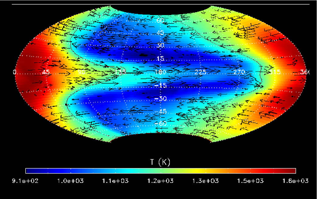
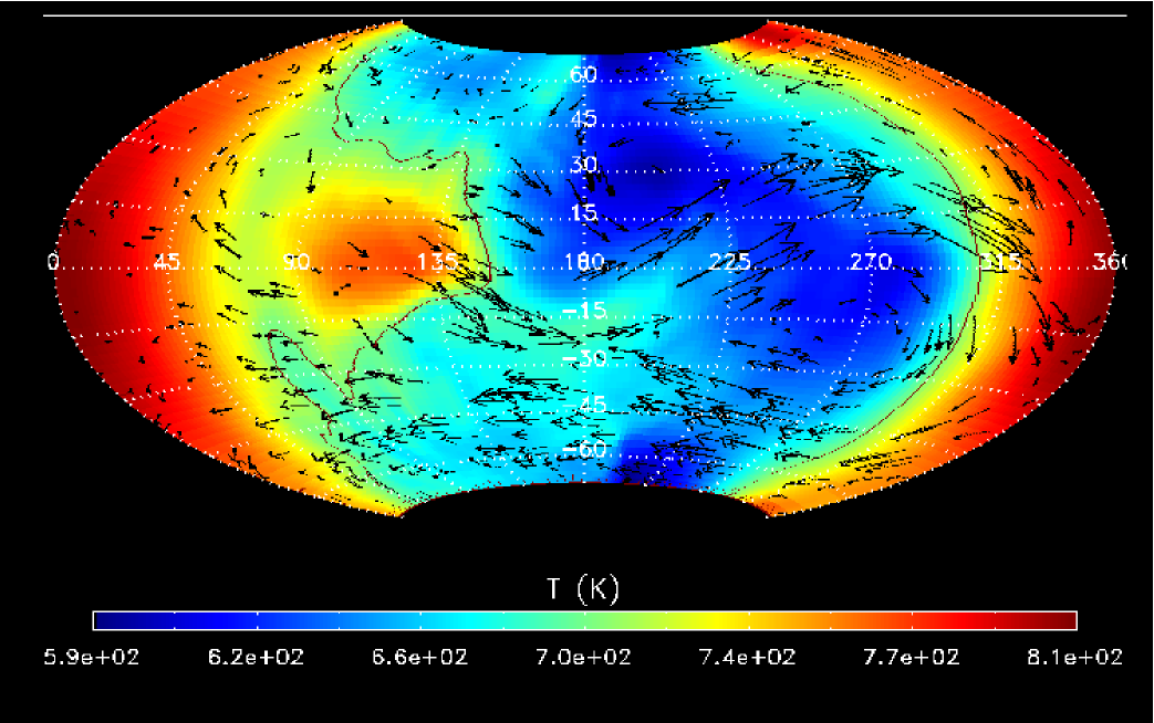
Figure 2: Temperature variations at the photosphere of planets with orbital periods of 1 (left panel) and 7 (right panel) days. Clear structures associated with stable jets are evident in the 1-day simulation, while the night-side temperature of the highly variable 7 day simulation is much more uniform.

The behavior of the simulation with an orbital period of $7$ days is somewhat different. In general the structure of an eastward equatorial jet and westward jets at higher and lower latitudes’ persists. However, the day-night temperature difference in this simulations is smaller. The jet velocity, driven by the temperature differential, is substantial smaller and the resulting temperature and velocity structure on the night-side is quite variable.

4 Decoupled Energy Equations: Temperature Inversions

As spectral observations become available for an increasing number of transiting planets, the presence of temperature inversions in several systems have become evident ([eg.][Burrows et al. (2007), Burrows et al. (2007)]). Although suggested by [Hubeny et al. (2003), Hubeny et al. (2003)], prior to these observations this notion had not been pursued. The physics behind this inversion can be understood in terms of the different opacities for optical and infrared photons. The opacity of the impinging stellar energy (optical) can be significantly different then the opacity of the reprocessed infrared radiation from the planet. Although a one-dimensional wavelength dependent radiative transfer model implicitly accounts for these effects by modelling the impinging stellar spectrum, full radiative hydrodynamical models must use average grey opacities due to computational considerations. In order to encapsulate this physics within a full hydrodynamical model I have calculated separate grey opacities for the incident stellar light and the reprocessed light. Both are still functions of the local temperature and pressure, but the stellar opacities are weighted toward optical wavelengths.

Furthermore, to allow for the inversion I have de-coupled the thermal and radiative energy components. Each can now evolve independently, though they are linked by the appropriate emission and absorption terms. Although computationally more intensive, this is a significant improvement to previously employed models. The thermal energy equation is given by

$$\left[{{\partial\epsilon}\over{\partial t}}+({\bf u}\cdot\nabla)\epsilon\right]=-P\,\nabla\cdot{\bf u}-\rho\kappa_{P}\left(T,P\right)\left[B\left(T\right)-cE_{R}\right]+\rho\kappa_{A}\left(T,P\right)F_{\star}e^{-\tau_{\star}},$$ (9)

while the independent radiation energy equation is given by

$${{\partial E_{R}}\over{\partial t}}+\nabla\cdot{\bf F}=\rho\kappa_{P}\left(T,P\right)\left[B\left(T\right)-cE_{R}\right].$$ (10)

As before, $\epsilon=c_{v}\rho T$ is the internal energy density, $T$ is the local gas temperature, and $c_{v}$ is the specific heat. In addition, $B\left(T\right)=4\sigma T^{4}$, $\kappa_{A}\left(T,P\right)$ is the absorption opacity averaged with the stellar temperature, and $F_{\star}$ is the impinging stellar flux. The term proportional to $B\left(T\right)-cE_{R},$ represents the exchange of energy between the thermal and radiative components through the emission and absorption of the lower energy photons. The $\rho\kappa_{A}\left(T,P\right)F_{\star}e^{-\tau_{\star}}$ term represents the higher energy stellar photons absorbed by the gas. Given the relatively low local temperatures, I do not consider the energy re-emitted into the higher energy waveband. The radiative flux is treated using the flux-limited diffusion method described in Equation (4). Equations (9) and (10) contain three separate opacities: the optical absorption opacity $\kappa_{A}$, the infrared Planck opacity $\kappa_{P}$, and the infrared Rosseland opacity $\kappa_{R}$ that appears through the flux term.

The effect of decoupling the energy equations and including 3 separate opacities can best be understood by considering the radiative behavior of Equations (9) and (10), ie. in the absence of dynamics. If we express the ratio of the stellar absorption opacity to the local opacity as ([Hubeny et al. (2003), Hubeny et al. (2003)])

$$\gamma^{4}\equiv\frac{\kappa_{A}\left(T,P\right)}{\kappa_{P}\left(T,P\right)},$$ (11)

then the steady-state, radial temperature profile can be expressed as

$$T^{4}(r)=\frac{\gamma^{4}(r)T_{0}^{4}e^{-\tau_{\star}}}{4}-\frac{E_{R}(r)}{a}.$$ (12)

The temperature in the upper atmosphere, near the stellar photosphere ($\tau_{\star}\sim 1$) will scale as $\gamma T_{0}$, where $T_{0}$ is the equilibrium stellar temperature at the planetary semi-major axis. The presence of an inversions thus becomes dependent on the radial structure of $\gamma$. In Figure (3) I show the solution to Equations (9) and (10) in the absence of dynamics. As expected, the inversion is high in the atmosphere, where $\gamma$ is around or above unity and $\tau_{\star}$ is small. Figure (3) clearly demonstrates how the thermal and radiative energies become de-coupled, requiring solving the equations separately. Full dynamical simulations are not presented here, but will be in explored in detail in [Dobbs-Dixon et al. (2008), Dobbs-Dixon & Lin (2008)].

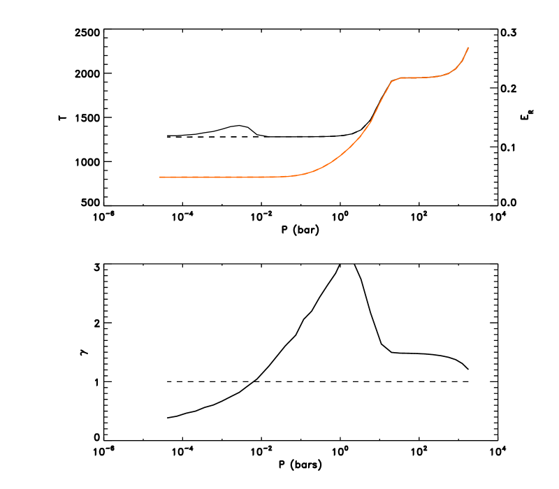
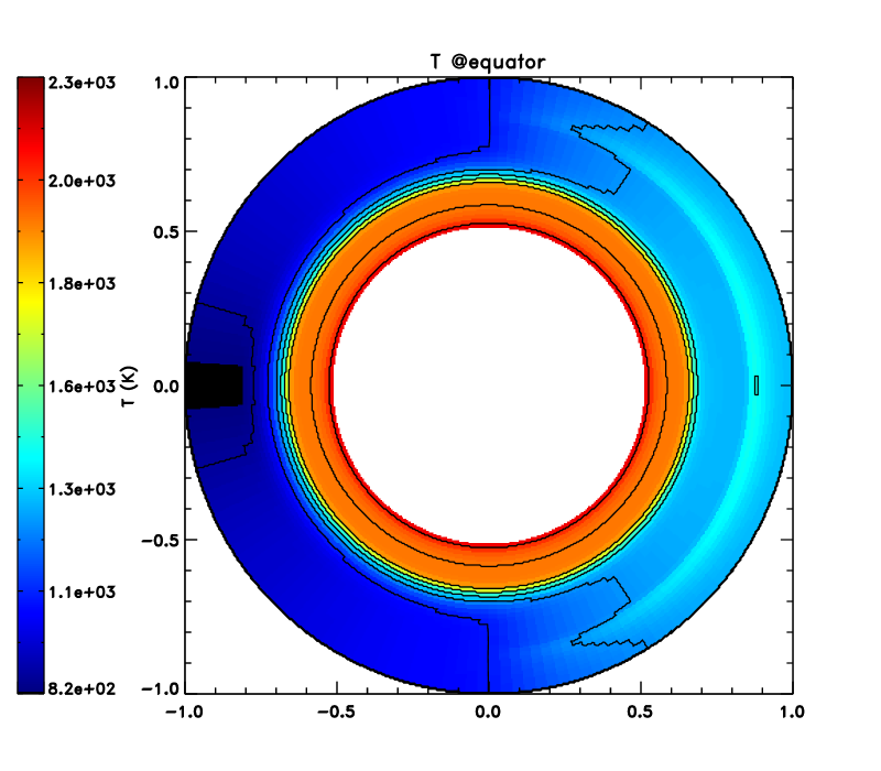
Figure 3: The temperature in HD 209458b concentrating only on the radiative solution to Equations (9) and (10). The left hand panel shows the temperature-pressure profile at the subsolar point. The inversion in T (solid line) is quite clear. The dashed line shows the decoupled radiative energy $E_{R}$. The orange line shows the temperature profile at the anti-stellar point. The lower left panel shows the behavior of $\gamma$ with pressure. The right panel shows the entire equatorial slice of the same simulation with the star to the right.

5 Discussion

In this proceeding I have reviewed results from full three-dimensional radiative hydrodynamical simulations of the atmospheres of close-in planets. Simulations for a range of atmospheric opacities and semi-major axis were performed. The results indicate that both stellar proximity and opacity are both crucial factors in determining the behavior of planetary atmospheres. Increasing planetary opacities yields less efficient advection and colder night-side temperatures. Furthermore, planets situated at 1 and 3 day orbital periods exhibit a fairly stable banded jet structure, with jet width increasing with rotation period. On the other-hand, dynamics of planets with 7 day orbital periods can be much more variable, with wandering jets and the formation of vortices on the night-side.

The decoupling of the thermal and radiative energies, as well as the introduction of multiple opacities relevant for impinging optical stellar photons vrs local re-radiated infrared photons allows us to explore in greater detail temperature structure near the top of the atmosphere. Radiative solutions presented in Section (4) produce temperature inversions similar to those observed and demonstrate the feasibility of simultaneously studying these radiative features and the resulting hydrodynamics. The existence of an inversion depends critically on the ratio of the optical to infrared opacities and the behavior of this ratio with radius.

Given the importance of both optical and infrared opacities it is fruitful to consider how we expect atmospheric properties to vary as we change these two quantities independently. [Fortney et al. (2008), Fortney et al. (2008)] suggested a classification planets based on the presence or absence of TiVO in the upper atmosphere. Although the presence of TiVO in the upper atmosphere is controversial, it would provide the necessary absorption opacity to cause an inversion. Fortney’s classifications of pM and pL classes correspond to those with and without detected inversions. Here extend this classification in terms of the individual absorption ($\kappa_{A}\left(T,P\right)$) and Planck ($\kappa_{P}\left(T,P\right)$)opacities explored in this proceeding.

As explained in Section (3), the night-side temperature is governed by the efficiency of advection, which in turn is determined by the cooling timescale where the incident radiation is deposited. The cooling timescale is directly related to the local Planck opacity $\kappa_{P}\left(T,P\right)$; large $\kappa_{P}\left(T,P\right)$ will result in a large day-night temperature differential. Such a distinction is observable from current and ongoing phase monitoring programs. On the other hand, the absorption opacity for the incident stellar light $\kappa_{A}\left(T,P\right)$ will play an important role in the presence or absence of a temperature inversion. As described in Section (4) the ratio $\gamma=(\frac{\kappa_{A}\left(T,P\right)}{\kappa_{P}\left(T,P\right)})^{1/4}$ will determine the temperature structure in the upper atmosphere. If the radial structure of $\gamma e^{-\tau_{\star}}$ is such that it peaks in the upper atmosphere there will be an inversion. In these terms, the presence of TiVO (a pL planet) would lead to large $\kappa_{A}\left(T,P\right)$, but an inversion would occur only if $\kappa_{P}\left(T,P\right)$ does not also increase. In Figure (4) I have unified these two concepts onto a single diagram. A measurement of both the magnitude of day-night temperature differential and a determination of the presence or absence of an inversion will uniquely tell you both the optical and infrared opacities and place the planet in one of the quadrants. Such a determination will ultimately tell us much about the formation and evolution of these planets.

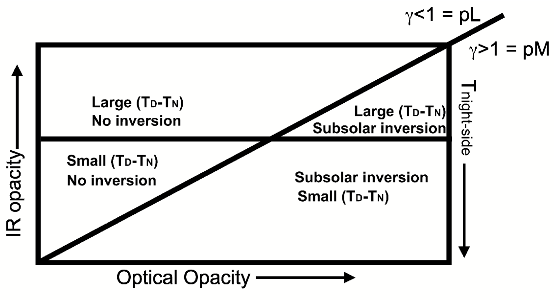
Figure 4: The gross behavior of irradiated atmospheres as you change the absorption and local Planck opacities. Increasing optical absorption opacity ($\kappa_{A}\left(T,P\right)$) is given in the horizontal axis, while the vertical axis gives the local opacity to re-radiated photons ($\kappa_{P}\left(T,P\right)$). The diagonal line demarcates the division between planets with an inversion ($\gamma>1$) and those without ($\gamma<1$), where $\gamma^{4}=\kappa_{A}\left(T,P\right)/\kappa_{P}\left(T,P\right)$. Phase measurements coupled to inversion determinations will uniquely place you in a given quadrant.

References

- [Alexander & Ferguson (1994)] Alexander, D.R. & Ferguson, J.W. 1994, ApJ, 437, 879-891
- [Burkert et al. (2005)] Burkert, A. Lin, D.N.C., Bodenheimer, P.H., Jones, C.A. & Yorke, H.W. 2005 ApJ, 618, 512-523
- [Burrows et al. (2007)] Burrows, A., Hubeny, I., Budaj, J., Knutson, H.A. & Charbonneau, D. ApJL 668, L171-L174
- [Dobbs-Dixon & Lin (2008)] Dobbs-Dixon, I., & Lin, D.N.C. 2008, ApJ, 673, 513
- [Dobbs-Dixon et al. (2008)] Dobbs-Dixon, I. et al. 2008, In Preparation
- [Fortney et al. (2008)] Fortney, J.J., Lodders, K., Marley, M.S. & Freedman, R.S. 2008, ApJ 678, 1419-1435
- [Freedman et al. (2008)] Freedman, R.S., Marley, M.S. & Lodders, K. 2008, ApJS, 174, 504-513
- [Hubeny et al. (2003)] Hubeny, I., Burrows, A. & Sudarsky, D. 2008, ApJ, 594, 1011-1018
- [Levermore & Pomraning (1981)] Levermore & Pomraning 1981, ApJ, 248, 321-334
- [Pollack et al. (1985)] Pollack, J.B., McKay, C.P. & Christofferson, B.M. 1985, Icarus, 64, 471-492
- [Showman et al (2008)] Showman, A.P., Cooper, C.S., Fortney, J.J. & Marley, M.S. 2008, ArXiv e-prints, 2008, 802