Bayesian Selection of sign $\mu$ within mSUGRA in Global Fits Including WMAP5 Results

Abstract:

We study the properties of the constrained minimal supersymmetric standard model (mSUGRA) by performing fits to updated indirect data, including the relic density of dark matter inferred from WMAP5. In order to find the extent to which $\mu<0$ is disfavoured compared to $\mu>0$, we compare the Bayesian evidence values for these models, which we obtain straightforwardly and with good precision from the recently developed multi–modal nested sampling (‘MultiNest’) technique. We find weak to moderate evidence for the $\mu>0$ branch of mSUGRA over $\mu<0$ and estimate the ratio of probabilities to be $P(\mu>0)/P(\mu<0)=6-61$ depending on the prior measure and range used. There is thus positive (but not overwhelming) evidence that $\mu>0$ in mSUGRA. The MultiNest technique also delivers probability distributions of parameters and other relevant quantities such as superpartner masses. We explore the dependence of our results on the choice of the prior measure used. We also use the Bayesian evidence to quantify the consistency between the mSUGRA parameter inferences coming from the constraints that have the largest effects: $(g-2)_{\mu}$, $BR(b\rightarrow s\gamma)$ and cold dark matter (DM) relic density $\Omega_{\mathrm{DM}}h^{2}$.

1 Introduction

The impending start of operation of the Large Hadron Collider (LHC) makes this a very exciting time for supersymmetric (SUSY) phenomenology. Numerous groups have been pursuing a programme to fit simple SUSY models and identify the regions in the parameter space that might be of interest with the forthcoming LHC data [1, 2, 3, 4, 5, 6]. The Minimal Supersymmetric Standard Model (MSSM) with one particular choice of universal boundary conditions at the grand unification scale, called either the Constrained Minimal Supersymmetric Standard Model (CMSSM) or mSUGRA [7], has been studied quite extensively in multi–parameter scans. mSUGRA has proved to be a popular choice for SUSY phenomenology because of the small number of free parameters. In mSUGRA, the scalar mass $m_{0}$, gaugino mass $M_{1/2}$ and tri–linear coupling $A_{0}$ are assumed to be universal at a gauge unification scale $M_{\rm GUT}\sim 2\times 10^{16}$ GeV. In addition, at the electroweak scale one selects $\tan\beta$, the ratio of Higgs vacuum expectation values and sign$(\mu)$, where $\mu$ is the Higgs/higgsino mass parameter whose square is computed from the potential minimisation conditions of electroweak symmetry breaking (EWSB) and the empirical value of the mass of the $Z^{0}$ boson, $M_{Z}$. The family universality assumption is well motivated since flavour changing neutral currents are observed to be rare. Indeed several string models (see, for example Ref. [8]) predict approximate MSSM universality in the soft terms. Nevertheless, mSUGRA is just one (albeit popular) choice among a multitude of possibilities.

Recently, Bayesian parameter estimation techniques using the Markov Chain Monte Carlo (MCMC) sampling have been applied to the study of mSUGRA, performing a multi–dimensional Bayesian fit to indirect constraints [9, 10, 11, 12, 13, 14, 15, 16]. Also, a study has been extended to large volume string compactified models [17]. A particularly important constraint comes from the cold dark matter (DM) relic density $\Omega_{\mathrm{DM}}h^{2}$ determined by the Wilkinson Microwave Anisotropy Probe (WMAP). DM is assumed to consist solely of the lightest supersymmetric particle (LSP). As pointed out in [12], the accuracy of the DM constraint results in very narrow steep regions of degenerate $\chi^{2}$ minima as the system is rather under–constrained. This makes the global fit to all the relevant mSUGRA parameters potentially difficult. If the MSSM is confirmed in the forthcoming collider data, it will hopefully be possible to break many of these degeneracies using collider observables such as edges in kinematical distributions. However, it is expected that one degeneracy will remain from LHC data in the form of the overall mass scale of the sparticles. We apply the newly developed MultiNest technique [18, 19] to explore this highly degenerate parameter space efficiently. With this technique, one can also calculate the ‘Bayesian evidence’ which plays the central role in Bayesian model selection and hence allows one to distinguish between different models.

Ref. [20] performed a random scan of $10^{5}$ points in the parameter spaces of mSUGRA, minimal anomaly mediated SUSY breaking (mAMSB) and minimal gauge mediated SUSY breaking (mGMSB). $b$ and electroweak physics observables (but not the dark matter relic density) were used to assign a $\chi^{2}$ to each of the points. The resulting minimum $\chi^{2}$ values for each scenario were then compared in order to select which model is preferred by the data. Unfortunately, the conclusions drawn (that mAMSB is preferred by data) may have been reversed had the dark matter relic density been included in the $\chi^{2}$ fit. It is also not clear how accurate the resulting value of minimum $\chi^{2}$ is in each scenario, since the scans are necessarily sparse due to the high dimensionality of the parameter space. Recently, several studies of the mSUGRA parameter space have used Markov Chain Monte Carlo in order to focus on the joint analysis of indirect constraints from experiment with the $\Omega_{\mathrm{DM}}h^{2}$ constraint as determined by WMAP and other data. We extend this approach by using MultiNest to calculate the Bayesian evidence, which, when compared with fits to different models, can be used for hypothesis testing. As an example, we consider $\mu>0$ mSUGRA versus $\mu<0$ mSUGRA as alternative hypotheses. In Ref. [12], the evidence ratio for these two quantities was calculated using the method of bridge sampling [21] in MCMCs. However, it is not clear how accurate the estimation of the evidence ratio was, and no uncertainties were quoted. The present approach yields, robustly small uncertainties on the ratio, for a given hypothesis and prior probability distribution. Since Ref. [12], a tension has developed between the constraints coming from the anomalous magnetic moment of the muon $(g-2)_{\mu}$, and the branching ratio of the decay of $b$ quarks into $s$ quarks $BR(b\rightarrow s\gamma)$, which favour opposite signs of $\mu$ [14]. Ref. [14] investigated the constraints on continuous parameters for either sign of $\mu$ and used the Bayesian calibrated p–value method [22] to get a rough estimate of the upper limit for the evidence ratio between $\mu>0$ mSUGRA and $\mu<0$ mSUGRA of $10:1$. We also use the evidence to examine quantitatively any incompatibilities between mSUGRA parameter inferences coming from three main constraints: $(g-2)_{\mu}$, $BR(b\rightarrow s\gamma)$ and $\Omega_{\mathrm{DM}}h^{2}$. Thus we determine to what extent the three measurements are compatible with each other in an mSUGRA context. We also update the fits to WMAP5 data for the first time and include additional $b$–physics constraints. Recent data point to an increased statistical significance in the discrepancy between the Standard Model prediction and the experimental value of $(g-2)_{\mu}$, and this leads to an additional statistical pull towards a larger contribution of $(g-2)_{\mu}$ coming from supersymmetry.

Our purpose in this paper is two–fold: as well as producing interesting physical insights, we also aim to gain experience in developing and applying tools for efficient Bayesian inference, which will prove useful in the analysis of future collider data.

This paper is organised as follows. In Section 2 we motivate the case for Bayesian model selection. In Section 3 we outline our theoretical setup and present our results in Section 4. Finally, in Section 5 we list the summary and present our conclusions. We motivate the case for the use of Bayesian evidence in quantifying consistency between different data–sets in Appendix A.

2 Bayesian Inference

A common problem in data analysis is to use the data to make inferences about parameters of a given model. A higher level of inference is to decide between two or more competing models. For instance, in the case of mSUGRA, one would like to know whether there is sufficient evidence in the data to rule out the $\mu<0$ branch. Bayesian inference provides a consistent approach to model selection as well as to the estimation of a set parameters $\mathbf{\Theta}$ in a model (or hypothesis) $H$ for the data $\mathbf{D}$. It can also be shown that Bayesian inference is the unique consistent generalisation of the Boolean algebra [23].

Bayes’ theorem states that

$$\Pr(\mathbf{\Theta}|\mathbf{D},H)=\frac{\Pr(\mathbf{D}|\,\mathbf{\Theta},H)\Pr(\mathbf{\Theta}|H)}{\Pr(\mathbf{D}|H)},$$ (1)

where $\Pr(\mathbf{\Theta}|\mathbf{D},H)\equiv P(\mathbf{\Theta})$ is the posterior probability distribution of the parameters, $\Pr(\mathbf{D}|\mathbf{\Theta},H)\equiv\mathcal{L}(\mathbf{\Theta})$ is the likelihood, $\Pr(\mathbf{\Theta}|H)\equiv\pi(\mathbf{\Theta})$ is the prior distribution, and $\Pr(\mathbf{D}|H)\equiv\mathcal{Z}$ is the Bayesian evidence.

Bayesian evidence is simply the factor required to normalise the posterior over $\mathbf{\Theta}$ and is given by:

$$\mathcal{Z}=\int{\mathcal{L}(\mathbf{\Theta})\pi(\mathbf{\Theta})}d^{N}\mathbf{\Theta},$$ (2)

where $N$ is the dimensionality of the parameter space. Since the Bayesian evidence does not depend on the parameter values $\mathbf{\Theta}$, it is usually ignored in parameter estimation problems and the posterior inferences are obtained by exploring the un–normalized posterior using standard MCMC sampling methods.

A useful feature of Bayesian parameter estimation is that one can easily obtain the posterior distribution of any function, $f$, of the model parameters $\mathbf{\Theta}$. Since,

$$\Pr(f|\mathbf{D})=\int{\Pr(f,\mathbf{\Theta}|\mathbf{D})d\mathbf{\Theta}}=\int{\Pr(f|\mathbf{\Theta},\mathbf{D})\Pr(\mathbf{\Theta}|\mathbf{D})d\mathbf{\Theta}}=\int{\delta(f(\mathbf{\Theta})-f)\Pr(\mathbf{\Theta}|\mathbf{D})d\mathbf{\Theta}}$$ (3)

where $\delta(x)$ is the delta function. Thus one simply needs to compute $f(\mathbf{\Theta})$ for every Monte Carlo sample and the resulting sample will be drawn from $\Pr(f|\mathbf{D})$. We make use of this feature in Section 4.2 where we present the posterior probability distributions of various observables used in the analysis of mSUGRA model.

In order to select between two models $H_{0}$ and $H_{1}$ one needs to compare their respective posterior probabilities given the observed data set $\mathbf{D}$, as follows:

$$\frac{\Pr(H_{1}|\mathbf{D})}{\Pr(H_{0}|\mathbf{D})}=\frac{\Pr(\mathbf{D}|H_{1})\Pr(H_{1})}{\Pr(\mathbf{D}|H_{0})\Pr(H_{0})}=\frac{\mathcal{Z}_{1}}{\mathcal{Z}_{0}}\frac{\Pr(H_{1})}{\Pr(H_{0})},$$ (4)

where $\Pr(H_{1})/\Pr(H_{0})$ is the prior probability ratio for the two models, which can often be set to unity but occasionally requires further consideration. It can be seen from Eq. 4 that the Bayesian evidence takes the center stage in Bayesian model selection. As the average of likelihood over the prior, the Bayesian evidence is higher for a model if more of its parameter space is likely and smaller for a model with highly peaked likelihood but has many regions in the parameter space with low likelihood values. Hence, Bayesian model selection automatically implements Occam’s razor: a simpler theory which agrees well enough with the empirical evidence is preferred. A more complicated theory will only have a higher evidence if it is significantly better at explaining the data than a simpler theory.

Unfortunately, evaluation of the multidimensional integral (2) is a challenging numerical task. Standard techniques like thermodynamic integration [24] are extremely computationally expensive which makes evidence evaluation typically at least an order of magnitude more costly than parameter estimation. Some fast approximate methods have been used for evidence evaluation, such as treating the posterior as a multivariate Gaussian centred at its peak (see e.g. Ref. [25]), but this approximation is clearly a poor one for multi–modal posteriors (except perhaps if one performs a separate Gaussian approximation at each mode). The Savage–Dickey density ratio has also been proposed [26] as an exact, and potentially faster, means of evaluating evidences, but is restricted to the special case of nested hypotheses and a separable prior on the model parameters. Bridge sampling [21] allows the evaluation of the ratio of Bayesian evidence of two models and is implemented in the ‘bank sampling’ method of Ref. [27] but it is not yet clear how accurately bank sampling can calculate these evidence ratios. Various alternative information criteria for model selection are discussed by [28], but the evidence remains the preferred method.

The nested sampling approach, introduced by Skilling [29], is a Monte Carlo method targeted at the efficient calculation of the evidence, but also produces posterior inferences as a by–product. Feroz & Hobson [18, 19] built on this nested sampling framework and have recently introduced the MultiNest algorithm which is efficient in sampling from multi–modal posteriors exhibiting curving degeneracies, producing posterior samples and calculating the evidence value and its uncertainty. This technique has greatly reduced the computational cost of model selection and the exploration of highly degenerate multi–modal posterior distributions. We employ this technique in this paper.

The natural logarithm of the ratio of posterior model probabilities provides a useful guide to what constitutes a significant difference between two models:

$$\log\Delta E=\log\left[\frac{\Pr(H_{1}|\mathbf{D})}{\Pr(H_{0}|\mathbf{D})}\right]=\log\left[\frac{\mathcal{Z}_{1}}{\mathcal{Z}_{0}}\frac{\Pr(H_{1})}{\Pr(H_{0})}\right].$$ (5)

We summarise convention we use in this paper in Table 1.

$|\log\Delta E|$	Odds	Probability	Remark
$<1.0$	$\lesssim 3:1$	$<0.750$	Inconclusive
$1.0$	$\sim 3:1$	$0.750$	Weak Evidence
$2.5$	$\sim 12:1$	$0.923$	Moderate Evidence
$5.0$	$\sim 150:1$	$0.993$	Strong Evidence

Table 1: The scale we use for the interpretation of model probabilities. Here the $\log$ represents the natural logarithm.

While for parameter estimation, the priors become irrelevant once the data are powerful enough, for model selection the dependence on priors always remains (although with more informative data the degree of dependence on the priors is expected to decrease, see e.g. Ref. [30]); indeed this explicit dependence on priors is one of the most attractive features of Bayesian model selection. Priors should ideally represent one’s state of knowledge before obtaining the data. Rather than seeking a unique ‘right’ prior, one should check the robustness of conclusions under reasonable variation of the priors. Such a sensitivity analysis is required to ensure that the resulting model comparison is not overly dependent on a particular choice of prior and the associated metric in parameter space, which controls the value of the integral involved in the computation of the Bayesian evidence (for some relevant cautionary notes on the subject see Ref. [31]).

One of the most important applications of model selection is to decide whether the introduction of new parameters is necessary. Frequentist approaches revolve around the significance test and goodness–of–fit statistics, where one accepts the additional parameter based on the improvement in $\Delta\chi^{2}$ by some chosen threshold. It has been shown that such tests can be misleading (see e.g. Ref. [26, 22]), not least because they depend only on the values of $\chi^{2}$ at the best–fit point, rather than over the entire allowed range of the parameters.

Another application of Bayesian model selection is in quantifying the consistency between two or more data sets or constraints [25, 32]. Different experimental observables may “pull” the model parameters in different directions and consequently favour different regions of the parameter space. Any obvious conflicts between the observables are likely to be noticed by the “chi by eye” method employed to date but it is imperative for forthcoming high–quality constraints to have a method that can quantify these discrepancies. The simplest scenario for analysing different constraints on a particular model is to assume that all constraints provide information on the same set of parameter values. We represent this hypothesis by $H_{1}$. This is the assumption which underlies the joint analysis of the constraints. However, if we are interested in accuracy as well as precision then any systematic differences between constraints should also be taken into account. In the most extreme case, which we represent by $H_{0}$, the constraints would be in conflict to such an extent that each constraint requires its own set of parameter values, since they are in different regions of parameter space. Bayesian evidence provides a very easy method of distinguishing between scenarios, $H_{0}$ and $H_{1}$. To see this, we again make use of Eq. 4. If we have no reason to favour either of $H_{0}$ or $H_{1}$ over the other, then we can distinguish between these two scenarios using the following ratio,

$$R=\frac{\Pr(\mathbf{D}|H_{1})}{\Pr(\mathbf{D}|H_{0})}=\frac{\Pr(\mathbf{D}|H_{1})}{\prod_{i}\Pr(D_{i}|H_{0})}.$$ (6)

Here the numerator represents the joint analysis of all the constraints $\mathbf{D}=\{D_{1},D_{2},\ldots,D_{n}\}$ while in the denominator the individual constraints $D_{1},D_{2},\ldots,D_{n}$ are assumed to be independent and are each fit individually to mSUGRA, with a different set of mSUGRA parameters for each $D_{i}$. The interpretation of the $\log R$ value can be made in a similar manner to model selection, as discussed in the preceding paragraph. A positive value of $\log R$ gives the evidence in favour of the hypothesis $H_{1}$ that all the constraints are consistent with each other while a negative value would point towards tension between constraints, which prefer different regions of mSUGRA parameter space. We follow this recipe to carry out consistency checks for the mSUGRA model between $(g-2)_{\mu}$, $BR(b\rightarrow s\gamma)$ and $\Omega_{\mathrm{DM}}h^{2}$ as determined by WMAP and other cosmological measurements. The $H_{1}$ hypothesis thus states that mSUGRA jointly fits these three observables, whereas $H_{0}$ states that they all prefer different regions of parameter space and so we require an ‘(mSUGRA)³’ model to fit them. Given the fact that Bayesian evidence naturally embodies a quantification of Occam’s razor, the resulting complexity in the model coming from the additional 2 sets of mSUGRA parameters must be matched by a better fit to data for $H_{0}$ to be preferred.

3 The Analysis

Our parameter space $\mathbf{\Theta}$ contains 8 parameters, 4 of them being the mSUGRA parameters; $m_{0}$, $M_{1/2}$, $A_{0}$, $\tan\beta$ and the rest taken from the Standard Model (SM): the QED coupling constant in the ${\overline{M}S}$ scheme $\alpha^{\overline{MS}}(M_{Z})$, the strong coupling constant $\alpha_{s}^{\overline{MS}}(M_{Z})$, the running mass of the bottom quark $m_{b}(m_{b})^{\overline{MS}}$ and the pole top mass $m_{t}$. We refer to these SM parameters as nuisance parameters. Experimental errors on the mass $M_{Z}$ of the $Z^{0}$ boson and the muon decay constant $G_{\mu}$ are so small that we fix these parameters to their central values of $91.1876$ GeV and $1.16637\times 10^{-5}$ GeV^-2 respectively.

For all the models analysed in this paper, we used 4,000 live points (see Refs. [18, 19]) with the MultiNest technique. This corresponds to around 400,000 likelihood evaluations taking approximately $20$ hours on 4 3.0 GHz Intel Woodcrest processors.

3.1 The Choice of Prior Probability Distribution

In all cases, we assume the prior is separable, such that

$$\pi(\mathbf{\Theta})=\pi(\theta_{1})\pi(\theta_{2})\ldots\pi(\theta_{8}),$$ (7)

where $\pi(\theta_{i})$ represents the prior probability of parameter $\theta_{i}$. We consider two initial ranges for the mSUGRA parameters which are listed in Table 2.

mSUGRA parameters	2 TeV range	4 TeV range
$m_{0}$	60 GeV to 2 TeV	60 GeV to 4 TeV
$M_{1/2}$	60 GeV to 2 TeV	60 GeV to 4 TeV
$A_{0}$	–4 TeV to 4 TeV	–7 TeV to 7 TeV
$\tan\beta$	2 to 62	2 to 62

Table 2: mSUGRA uniform prior parameter ranges

The “2 TeV” range is motivated by a general “naturalness” argument that SUSY mass parameters should lie within $\mathcal{O}(1$ TeV), since otherwise a fine-tuning in the electroweak symmetry breaking sector results. Deciding which region of parameter space is natural is obviously subjective. For this reason, we include the “4 TeV” range results to check the dependence on prior ranges. We consider the branches $\mu<0$ and $\mu>0$ separately.

SM parameters	Mean value	Uncertainty	Reference
	$\mu$	$\sigma$ (exp)
$1/\alpha^{\overline{MS}}$	$127.918$	$0.018$	[33]
$\alpha_{s}^{\overline{MS}}(M_{Z})$	$0.1176$	$0.002$	[33]
$m_{b}(m_{b})^{\overline{MS}}$	$4.20$ GeV	$0.07$ GeV	[33]
$m_{t}$	$170.9$ GeV	$1.8$ GeV	[34]

Table 3: Constraints on the Standard Model (nuisance) parameters

We impose flat priors on all 4 mSUGRA parameters (i.e. $m_{0},M_{1/2},A_{0}$ and $\tan\beta$) for the “2 TeV” and “4 TeV” ranges and both signs of $\mu$. Current constraints on SM (nuisance) parameters are listed in Table 3. With the means and $1\sigma$ uncertainties from Table 3, we impose Gaussian priors on SM (nuisance) parameters truncated at $4\sigma$ from their central values. We also perform the analysis for flat priors in $\log m_{0}$ and $\log M_{1/2}$ for both ranges and both signs of $\mu$. Since,

$$\int d\log m_{0}\ d\log M_{1/2}\ p(m_{0},M_{1/2}|{\bf D})=\int{dm_{0}}\ dM_{1/2}\ \frac{p(m_{0},M_{1/2}|{\bf D})}{m_{0}M_{1/2}}$$ (8)

it is clear that the logarithmic prior measures have a factor $1/(m_{0}M_{1/2})$ compared to the linear prior measure and so it could potentially favour lighter sparticles. If the data constrains the model strongly enough, lighter sparticles would only be favoured negligibly. Our main motive in seeing the variation of the fit to the variation in prior measure is to check the dependence of our results on the choice of the prior. For robust fits, which occur when there is enough precisely constraining data, the posterior probability density should only have a small dependence upon the precise form of the prior measure.

3.2 The Likelihood

Observable	Mean value	Uncertainty	Reference
${\delta a_{\mu}}\times 10^{-10}$	$29.5$	$8.8$	[36]
$M_{W}$	$80.398$ GeV	$27$ MeV	[37, 38]
$\sin^{2}\theta_{w}^{l}$	$0.23149$	$0.000173$	[39, 37]
$BR(b\rightarrow s\gamma)\times 10^{4}$	$3.55$	$0.72$	[40, 41]
$\Delta_{o-}$	$0.0375$	$0.0289$	[40, 41]
$R_{BR(B_{u}\rightarrow\tau\nu)}$	$1.259$	$0.378$	[42]
$R_{\Delta_{m_{s}}}$	$0.85$	$0.12$	[42, 43]

Table 4: Summary of the Gaussian distributed observables used in the analysis. For each quantity we use a likelihood function with central mean $\mu$ and standard deviation $s=\sqrt{\sigma^{2}+\tau^{2}}$ where $\sigma$ is the experimental uncertainty and $\tau$ is the theoretical uncertainty. $\Delta_{o-}$ represents the isospin asymmetry of $B\rightarrow K^{*}\gamma$. $R_{BR(B_{u}\rightarrow\tau\nu)}$ represents the ratio of the experimental and SM predictions of the branching ratio of $B_{u}$ mesons decaying into a tau and a tau neutrino. $R_{\Delta_{m_{s}}}$ is the ratio of the experimental and the SM neutral $B_{s}$ meson mixing amplitudes. The non-Gaussian likelihoods for the LEP constraint on Higgs mass, $BR(B_{s}\rightarrow\mu^{+}\mu^{-})$ and $\Omega_{\mathrm{DM}}h^{2}$ are described later.

Our calculation of the likelihood closely follows Ref. [15], with updated data and additional variables included, and is summarised in Table 4 and discussed further below. We assume that the measurements $D_{i}$ of observables (the ‘data’) used in our likelihood calculation are independent and have Gaussian errors, so that the likelihood distribution for a given model ($H$) is

$$\mathcal{L}(\mathbf{\Theta})\equiv\Pr(\mathbf{D}|\mathbf{\Theta},H)=\prod_{i}\Pr(D_{i}|\mathbf{\Theta},H),$$ (9)

where

$$\Pr(D_{i}|\mathbf{\Theta},H)=\frac{1}{\sqrt{2\pi\sigma_{i}^{2}}}\exp[-\chi^{2}/2]$$ (10)

and

$$\chi^{2}=\frac{(c_{i}-p_{i})^{2}}{\sigma_{i}^{2}}.$$ (11)

$p_{i}$ is the “predicted” value of the observable $i$ given the knowledge of the model $H$ and $\sigma$ is the standard error of the measurement.

In order to calculate predictions $p_{i}$ for observables from the input parameters $\mathbf{\Theta}$, SOFTSUSY2.0.17 [44] is first employed to calculate the MSSM spectrum. Bounds upon the sparticle spectrum have been updated and are based upon the bounds collected in Ref. [11]. Any spectrum violating a 95$\%$ limit from negative sparticle searches is assigned a zero likelihood density. Also, we set a zero likelihood for any inconsistent point, e.g. one which does not break electroweak symmetry correctly, has a charged LSP, or has tachyonic sparticles. For points that are not ruled out, we then link the mSUGRA spectrum via the SUSY Les Houches Accord [45] (SLHA) to various other computer codes that calculate various observables. For instance, micrOMEGAs1.3.6 [46], calculates $\Omega_{\mathrm{DM}}h^{2}$, the branching ratio $BR(B_{s}\rightarrow\mu^{+}\mu^{-})$ and the anomalous magnetic moment of the muon $(g-2)_{\mu}$.

The anomalous magnetic moment of the muon $a_{\mu}\equiv(g-2)_{\mu}/2$ was measured to be $a^{\mathrm{\mathrm{exp}}}_{\mu}=(11659208.0\pm 6.3)\times 10^{-10}$ [47]. Its experimental value is in conflict with the SM predicted value $a_{\mu}^{\mathrm{SM}}=(11659178.5\pm 6.1)\times 10^{-10}$ from [36], which includes the latest QED [48], electroweak [49], and hadronic [36] contributions to $a^{\mathrm{SM}}_{\mu}$. This SM prediction does not however account for $\tau$ data which is known to lead to significantly different results for $a_{\mu}$, implying underlying theoretical difficulties which have not been resolved so far. Restricting to $e^{+}e^{-}$ data, hence using the numbers given above, we find

$$\delta\frac{(g-2)_{\mu}}{2}\equiv\delta a_{\mu}\equiv a_{\mu}^{\mathrm{exp}}-a_{\mu}^{\mathrm{SM}}=(29.5\pm 8.8)\times 10^{-10}.$$ (12)

This excess may be explained by a supersymmetric contribution, the sign of which is identical in mSUGRA to the sign of the super potential $\mu$ parameter [50]. After obtaining the one-loop MSSM value of $(g-2)_{\mu}$ from micrOMEGAs v1.3.6, we add the dominant 2-loop corrections detailed in Refs. [51, 52].

The $W$ boson pole mass $M_{W}$ and the effective leptonic mixing angle $\sin^{2}\theta^{l}_{w}$ are also used in the likelihood. We take the measurements to be [37, 39]

$$M_{W}=80.398\pm 0.027\mbox{~{}GeV},\qquad\sin^{2}\theta_{w}^{l}=0.23149\pm 0.000173,$$ (13)

where experimental errors and theoretical uncertainties due to missing higher–order corrections in SM [53] and MSSM [38, 54] have been added in quadrature. The most up to date MSSM predictions for $M_{W}$ and $\sin^{2}\theta_{w}^{l}$ [38] are finally used to compute the corresponding likelihoods.

A parameterisation of the LEP2 Higgs search likelihood for various Standard Model Higgs masses is utilised, since the lightest Higgs $h$ of mSUGRA is very SM-like once the direct search constraints are taken into account. It is smeared with a 2 GeV assumed theoretical uncertainty in the SOFTSUSY2.0.17 prediction of $m_{h}$ as described in [13].

The experimental value of the rare bottom quark branching ratio to a strange quark and a photon $BR(b\rightarrow s\gamma)$ is constrained to be [55]

$$BR(b\rightarrow s\gamma)=(3.55\pm 0.26)\times 10^{-4}.$$ (14)

The SM prediction has recently moved down quite substantially from $(3.60\pm 0.30)\times 10^{-4}$ to $(3.15\pm 0.23)\times 10^{-4}$ [56, 57]. This shift was caused by including most of the next-to-next-to-leading order (NNLO) perturbative QCD contributions as well as the leading non-perturbative and electroweak effects. We use the publicly available code SuperIso2.0 [40] (linked via the SLHA to the mSUGRA spectrum predicted) which computes $BR(b\rightarrow s\gamma)$ in the MSSM with Minimal Flavor Violation. We note that mSUGRA is of such a minimal flavor violating form, and so the assumptions present in SuperIso2.0 are the appropriate ones. The computation takes into account one-loop SUSY contributions, as well as $\tan\beta$-enhanced two-loop contributions in the effective lagrangian approach. The recent partial NNLO SM QCD corrections are also included by the program. Ref. [41] derives a 95% interval for the bounds including the experimental and theory SM/MSSM errors to be

$$2.07\times 10^{-4}<BR(b\rightarrow s\gamma)<4.84\times 10^{-4}.$$ (15)

For the constraint on $BR(b\rightarrow s\gamma)$, we use the mean value of $3.55\times 10^{-4}$ and derive the 1–$\sigma$ uncertainty from the above given bound to be equal to $0.72\times 10^{-4}$. We note that this is twice as large as the uncertainty used in another recent global fit [14], where an enhancement in the posterior density of the large $\tan\beta$ region was observed to result from the new constraint.

The new upper 95$\%$ C.L. bound on $BR(B_{s}\rightarrow\mu^{+}\mu^{-})$ coming from the CDF collaboration is 5.8$\times 10^{-8}$. We are in possession [58] of the empirical $\chi^{2}$ penalty for this observable as a function of the predicted value of $BR(B_{s}\rightarrow\mu^{+}\mu^{-})$ from old CDF data when the 95$\%$ C.L. upper bound was 0.98$\times 10^{-8}$. Here, we assume that the shape of the likelihood penalty coming from data is the same as presented in Ref. [12], but that only the normalisation of the branching ratio shifts by the ratio of the 95$\%$ C.L. upper bounds: $0.58/0.98$.

For the $\Delta_{o-}$, isospin asymmetry of $B\rightarrow K^{*}\gamma$, the 95% confidence level for the experimental results from the combined BABAR and Belle data combined with the theoretical errors is [41]:

$$-0.018\times 10^{-4}<\Delta_{o-}<0.093\times 10^{-4},$$ (16)

with the central value of $0.0375$. We derive the 1–$\sigma$ uncertainty from the above given bound to be equal to $0.0289$. We use the publicly available code SuperIso2.0 [40] to calculate $\Delta_{o-}$. We neglect experimental correlations between the measurements of $\Delta_{o-}$ and $BR(b\rightarrow s\gamma)$. In practice, the $\Delta_{o-}$ constraint makes a much smaller difference than $BR(b\rightarrow s\gamma)$ to our fits, and so we expect the inclusion of a correlation to also have a small effect. The parametric correlations caused by variations of $\alpha_{s}(M_{Z})$ and $m_{b}(m_{b})$ are included by our analysis, since they are varied as input parameters.

The average experimental value of $BR(B_{u}\rightarrow\tau\nu)$ from HFAG [42] (under purely leptonic modes) is:

$$BR^{\mathrm{exp}}(B_{u}\rightarrow\tau\nu)=(141\pm 43)\times 10^{-6}.$$ (17)

The SM prediction is rather uncertain because of two incompatible empirically derived values of $|V_{ub}|$: one being $(3.68\pm 0.14)\times 10^{-3}$. The other comes from inclusive semi-leptonic decays and is $(4.49\pm 0.33)\times 10^{-3}$. These lead to $BR(B_{u}\rightarrow\tau\nu)$ values of $(0.85\pm 0.13)\times 10^{-4}$ and $(1.39\pm 0.44)\times 10^{-4}$ respectively. We statistically average these two by averaging the central values, and then adding the errors in quadrature and dividing by $\sqrt{2}$. This gives:

$$BR^{\mathrm{SM}}(B_{u}\rightarrow\tau\nu)=(112\pm 25)\times 10^{-6}.$$ (18)

Taking the ratio of the experimental and SM values of $BR(B_{u}\rightarrow\tau\nu)$ gives:

$$R_{BR(B_{u}\rightarrow\tau\nu)}=1.259\pm 0.378.$$ (19)

For the MSSM prediction, we use the formulae in Ref. [59], which include the large $\tan\beta$ limit of one-loop corrections coming from loops involving a charged Higgs.

The experimental and SM-predicted values of the neutral $B_{s}$ meson mixing amplitude are [42, 43]:

$$\Delta^{\mathrm{exp}}m_{s}=17.77\pm 0.12\mbox{~{}ps}^{-1},\Delta^{\mathrm{SM}}m_{s}=20.9\pm 2.6\mbox{~{}ps}^{-1}.$$ (20)

Taking the ratio of these two values, we get:

$$R_{\Delta m_{s}}=0.85\pm 0.12.$$ (21)

We use the formulae of Ref. [60] for the MSSM prediction of $R_{\Delta m_{S}}$, calculating it in the large $\tan\beta$ approximation. The dominant correction comes from one-loop diagrams involving a neutral Higgs boson.

Figure 1: Depiction of our likelihood constraint on the predicted value of $\Omega_{\mathrm{DM}}h^{2}$ due to lightest neutralinos, compared to a simple Gaussian with WMAP5 central value and a 1$\sigma$ uncertainty of 0.02.

The WMAP 5–year data combined with the distance measurements from the Type Ia supernovae (SN) and the Baryon Acoustic Oscillations (BAO) in the distribution of galaxies gives the $\Lambda$-cold dark matter fitted value of the dark matter relic density [61]:

$$\Omega\equiv\Omega_{\mathrm{DM}}h^{2}=0.1143\pm 0.0034.$$ (22)

In the present paper, we assume that the dark matter consists of neutralino, the LSP. Recently, it has been shown that the LSP relic density is highly sensitive to the pre-Big Bang Nucleosynthesis (BBN) rate and even a modest modification can greatly enhance the calculated relic density with no contradiction with the cosmological observations [62]. It is also possible that a non-neutralino component of dark matter is concurrently present and indeed the inclusion of neutrino masses via right-handed neutrinos can change the relic density prediction somewhat [63]. We therefore penalise only for the predicted $\Omega_{\mathrm{DM}}h^{2}$ being greater than the WMAP5 + BAO + SN central value. We define $x$ to be the predicted value of $\Omega_{\mathrm{DM}}h^{2}$, $c=0.1143$ to be the central $\Omega_{\mathrm{DM}}h^{2}$ value from WMAP5 + BAO + SN observations and $s$ to be the error on the predicted $\Omega_{\mathrm{DM}}h^{2}$ value which includes theoretical as well as experimental components. We take $s=0.02$ in order to incorporate an estimate of higher order uncertainties in its prediction [64] and we define the likelihood as:

$$\mathcal{L}(x\equiv\Omega_{\mathrm{DM}}h^{2})=\begin{cases}\frac{1}{c+\sqrt{\pi s^{2}/2}},&\mbox{if $x<c$}\\ \frac{1}{c+\sqrt{\pi s^{2}/2}}\exp\left[-\frac{(x-c)^{2}}{2s^{2}}\right],&\mbox{if $x\geq c$}.\\ \end{cases}$$ (23)

A diagram of the resulting likelihood penalty is displayed in Fig. 1. This differs slightly from the formulation suggested previously by one of the authors, for $\mathcal{L}(x\equiv\Omega_{\mathrm{DM}}h^{2})$ for the case when a non-neutralino component of dark matter is concurrently present, which drops more quickly than our flat likelihood up until the peak of WMAP Gaussian likelihood distribution.

4 Results

In this section, we first show our main results on the quantification of the preference of the fits for $\mu>0$. Next, we show some highlights of updated parameter constraints coming from the fit, finishing with a study on the level of compatibility of various observables.

4.1 Model Comparison

We summarise our main results in Table 5 in which we list the posterior model probability odds, $P_{+}/P_{-}$ for mSUGRA models with $\mu>0$ and $\mu<0$, for the two prior ranges used with flat and logarithmic prior measures as discussed in Section 3. The calculation of the ratio of posterior model probabilities requires the prior probability ratio for the two signs of $\mu$ (see Section 2), which we have set to unity. One could easily calculate the ratio $P_{+}/P_{-}$ for a different prior probability ratio $r$, by multiplying $P_{+}/P_{-}$ in Table 5 with $r$. From the probability odds listed in Table 5, although there is a positive evidence in favour of mSUGRA model with $\mu>0$, the extent of the preference depends quite strongly on the priors used and the evidence ranges from being relatively strong in the case of logarithmic prior with “$2$ TeV” range to weak for flat priors with “$4$ TeV” range. This dependence on the prior is a clear sign that the data are not yet of sufficiently high quality to be able to distinguish between these models unambiguously. Hopefully, the forthcoming high-quality data from LHC would be able to cast more light on it.

Prior	“2 TeV”		“4 TeV”
	flat	log	flat	log
$\log\Delta E$ (our determination)	$2.7\pm 0.1$	$4.1\pm 0.1$	$1.8\pm 0.1$	$3.2\pm 0.1$
$P_{+}/P_{-}$ (our determination)	$15.6\pm 1.1$	$61.6\pm 4.3$	$5.9\pm 0.4$	$24.0\pm 1.7$
$\log\Delta E$ (from Ref. [12])	$2.1$	$-$	$1.8$	$2.7$
$P_{+}/P_{-}$ (from Ref. [12])	$8.3$	$-$	$6.2$	$14.3$

Table 5: The posterior probability ratios for mSUGRA model with different signs of $\mu$. Here we have assumed the prior probabilities of the different signs of $\mu$ to be same. The uncertainties on $\log\Delta E$ for mSUGRA model with different signs of $\mu$ are the same for different priors, since with the MultiNest technique, the uncertainty on the evidence value is set by the number of live points and the stopping criteria (see Refs. [18, 19]) which were the same for different priors used in this study. The second row shows, for comparison, a previous determination with earlier data using the much less precise bridge sampling method. Some aspects of this fit were somewhat different to the present work’s approach and are discussed in the text.

We also show in Table 5 for comparison, the probability ratio $P_{+}/P_{-}$ determined in an earlier MCMC fit using different data [12]. We can see that our determination of the probability ratio favours $\mu>0$ more strongly than Ref. [12]. The main factors affecting this are that Ref. [12] had an anomalous magnetic moment of the muon less in conflict with experiment: $\delta a_{\mu}=(22\pm 10)\times 10^{-10}$ as opposed to Eq. 12 in the present analysis, which also includes the additional $b$-observables: $\Delta m_{s}$, $BR(B_{u}\rightarrow\tau\nu)$ and $\Delta_{0-}$. Some other details of the fit were also different in Ref. [12]: for instance $M_{1/2}<2$ TeV for all fits, and the range of $A_{0}$ was different. These ranges will affect the evidence obtained, at least to some degree. Unfortunately, Ref. [12] neglects to present statistical errors in the determination of the ratios of evidence values, a situation which is rectified in Table 5. It is clear from Table 5 that the uncertainty in the result of the model comparison is presently dominated by the prior choice, rather than by the small statistical uncertainty in the determination of the evidence ratio with MultiNest. It can however be concluded that present data favour the $\mu>0$ branch of mSUGRA with a Bayesian evidence going from weak to moderate, depending on the choice of prior.

To quantify the extent to which these results depend on $(g-2)_{\mu}$ constraint, we calculate the Bayesian evidence ratio, for mSUGRA models with $\mu>0$ and $\mu<0$, for the flat “4 TeV” range priors with all the observables discussed in Section 3.2 apart from $(g-2)_{\mu}$. We find $\log\Delta E=-0.5\pm 0.1$ translating into posterior probability odds $P_{+}/P_{-}=0.6\pm 1.1$. This shows that in the absence of $(g-2)_{\mu}$ constraint, both mSUGRA models with $\mu>0$ and $\mu<0$ are equally favoured by the data. Inclusion of $(g-2)_{\mu}$ constraint causes a shift of 2.3 $\log$ units in favour of $\mu>0$ for the linear “4 TeV” range prior measure and hence it can be concluded that $(g-2)_{\mu}$ does indeed dominate our model selection results in favour of $\mu>0$.

4.2 Updated Parameter Constraints

\psfrag{m12}{$m_{1/2}$ (TeV)}\psfrag{m0}{$m_{0}$ (TeV)}\psfrag{A0}{$A_{0}$ (TeV)}\psfrag{tanb}{$\tan\beta$}\includegraphics[width=173.44534pt,height=173.44534pt]{FIGS/pmf_m0_m12.ps}

\psfrag{m12}{$m_{1/2}$ (TeV)}\psfrag{m0}{$m_{0}$ (TeV)}\psfrag{A0}{$A_{0}$ (TeV)}\psfrag{tanb}{$\tan\beta$}\includegraphics[width=173.44534pt,height=173.44534pt]{FIGS/pmf_m0_tanb.ps}

\psfrag{m12}{$m_{1/2}$ (TeV)}\psfrag{m0}{$m_{0}$ (TeV)}\psfrag{A0}{$A_{0}$ (TeV)}\psfrag{tanb}{$\tan\beta$}\includegraphics[width=303.53267pt,height=21.68231pt]{FIGS/colormap.eps}

Figure 2: The 2-dimensional posterior probability densities in the plane spanned by mSUGRA parameters: $m_{0}$, $m_{1/2}$, $A_{0}$ and $\tan\beta$ for the linear prior measure “4 TeV” range analysis and $\mu>0$. The inner and outer contours enclose $68$% and $95$% of the total probability respectively. All of the other parameters in each plane have been marginalised over.

We display the results of the MultiNest fits on the $m_{0}-M_{1/2}$ and $m_{0}-\tan\beta$ plane posterior probability densities in Fig. 2 . Previous global fits in mSUGRA have found that the dark matter relic density has the largest effect on parameter space [9]. In particular, regions where the LSP annihilates efficiently through some particular mechanism are preferred by the fits. In the left-hand panel, we see that the highest posterior region is where the stau co-annihilation channel is active at the lowest value of $m_{0}$, where the lightest stau co-annihilates very efficiently with the lightest neutralino due to their near mass degeneracy. Next, in the approximate region 0.5 TeV $<m_{0}<$ 1.5 TeV, there is another reasonably high posterior region. In this region, $\tan\beta$ is large and the LSP is approximately half the mass of the pseudo-scalar Higgs boson $A^{0}$. The process $\chi_{1}^{0}\chi_{1}^{0}\rightarrow A^{0}\rightarrow b{\bar{b}}$ becomes an efficient channel in this region. For higher values of $m_{0}>2$ TeV, the hyperbolic branch [65, 66] régime reigns, where the LSP contains a significant higgsino component and annihilation into weak gauge boson pairs becomes quite efficient. This region dominantly has $\tan\beta>10$, as can be seen in the right-hand panel of Fig. 2. All of the qualitative features of previous MCMC global fits [9, 11, 12, 13, 15] have been reproduced in the figure, providing a useful validation of the MultiNest technique in a particle physics context, where the shape of the multi-dimensional posterior exhibits multi-modality and curving degeneracies. 2-dimensional marginalisations in other mSUGRA parameter combinations also agree to a large extent with previous MCMC fits, for both $\mu>0$ and $\mu<0$. However, compared to MCMC fits in Refs. [9, 11, 14], there has been a slight migration for $\mu>0$: the stau co-annihilation region has become relatively more favoured than previously and the hyperbolic branch has become less favoured. This is primarily due to $M_{W}$ and $\sin^{2}\theta_{w}^{l}$: our calculation includes 2-loop MSSM effects and so we are able to place smaller errors on the theoretical prediction than Refs. [9, 11, 14]. Both of these variables show a mild preference for a sizable SUSY contribution once these 2-loop effects are included [67]. The pure SOFTSUSY2.0.17 calculation is at 1-loop order and without the additional two loop effects, it displays a preference for larger SUSY scalar masses [12], thus favouring the hyperbolic branch region more. An effect in the opposite direction that comes from including the NNLO corrections to $BR(b\rightarrow s\gamma)$ is possible [14]. Large values of $m_{0}$ in the hyperbolic branch region lead to fairly light charged Higgs’ in mSUGRA due to charged Higgs-top loops, which may then push the branching ratio toward its experimentally preferred range, by adding constructively to the Standard Model contribution. However, our estimate of the combined statistical error of $BR(b\rightarrow s\gamma)$ in Table 4 means that this effect only has a small statistical pull on the fits, being out-weighed by the effects mentioned above in the opposite direction. We note here that, as $m_{t}$ as determined from experiment increases, the focus point region moves to higher values of $m_{0}$ [68]. However, very similar fits to the ones presented here were performed for $m_{t}=172.6\pm 1.8$ GeV, see Fig. 2a of Ref. [16], and the posterior density on the $m_{0}-M_{1/2}$ plane did not change much compared to the present paper (which uses $m_{t}=170.9\pm 1.8$ GeV).

\psfrag{m12}{$m_{1/2}$ (TeV)}\psfrag{mhalf}{$m_{1/2}$ (TeV)}\psfrag{m0}{$m_{0}$ (TeV)}\psfrag{A0}{$A_{0}$ (TeV)}\psfrag{tanb}{$\tan\beta$}\includegraphics[width=173.44534pt]{FIGS/nlf_m0_m12.ps}

\psfrag{m12}{$m_{1/2}$ (TeV)}\psfrag{mhalf}{$m_{1/2}$ (TeV)}\psfrag{m0}{$m_{0}$ (TeV)}\psfrag{A0}{$A_{0}$ (TeV)}\psfrag{tanb}{$\tan\beta$}\includegraphics[width=173.44534pt]{FIGS/nll_m0_m12.ps}

\psfrag{m12}{$m_{1/2}$ (TeV)}\psfrag{mhalf}{$m_{1/2}$ (TeV)}\psfrag{m0}{$m_{0}$ (TeV)}\psfrag{A0}{$A_{0}$ (TeV)}\psfrag{tanb}{$\tan\beta$}\includegraphics[width=303.53267pt,height=21.68231pt]{FIGS/colormap.eps}

Figure 3: The 2-dimensional mSUGRA posterior probability densities in the plane $m_{0}$, $m_{1/2}$ for $\mu<0$ for (left) the ‘4 TeV range’ linear measure prior analysis and (right) the ‘4 TeV range’ logarithmic measure prior analysis. The inner and outer contours enclose $68$% and $95$% of the total probability respectively. All of the other parameters in each plane have been marginalised over.

For $\mu<0$, the fit prefers a higher posterior probability for the focus point region compared to Ref. [12]. We show the marginalisation of $\mu<0$ mSUGRA to the $m_{0}-m_{1/2}$ plane in Fig. 3. The left-hand panel shows the linear measure prior analysis and may be compared directly with Fig. 5a of Ref. [12], which has the stau co-annihilation region having the highest posterior density. The increased discrepancy of $(g-2)_{\mu}$ in the present fit with current data will favour heavier sparticles due to the SUSY contribution being of the wrong sign for $\mu<0$ mSUGRA. In the right-hand side, we see how the fit changes due to a logarithmic measure on the prior. Indeed, the foreseen shift toward lower values of $m_{0}$ is significant, the stau co-annihilation channel being favoured once more. Although there are some similarities with the left-hand panel, it is clear that the choice of prior measure still has a non-negligible effect on the fit despite the inclusion of new $b$-physics observables.

Figure 4: Comparison of $\mu<0$ and $\mu>0$ 1-dimensional relative posterior probability densities of mSUGRA parameters for the linear measure prior ‘4 TeV’ range analysis. All of the other input parameters have been marginalised over.

With this fact still in mind, we compare the posterior probability density function for $\mu>0$ and $\mu<0$ in Fig. 4 for linear measure priors. In Fig. 4, we see the preference for heavier sparticles in the $\mu<0$ case reflected in the larger values for the universal scalar and gaugino masses $m_{0}$ and $m_{1/2}$. It is clear from the top left hand panel that any inference made about scalar masses $\mu<0$ will be quite sensitive to the exact range taken, since the $m_{0}$ distribution is near its maximum at large values close to 4 TeV. On the other hand, the data constrains $m_{1/2}<2$ TeV robustly. $\mu<0$ favours large $\tan\beta$ less than $\mu>0$ since for large $\tan\beta$, $(g-2)_{\mu}$ becomes more negative, with the wrong sign compared to the data.

Figure 5: An illustration of tensions between different observables for the mSUGRA model. The black (dash-dotted), red (thin solid) and the blue (thick solid) lines show the relative posterior probability for $\mu>0$, $\mu<0$ and the likelihood respectively for each observable.

	$\mu>0$		$\mu<0$
Parameter	$68$% region	$95$% region	$68$% region	$95$% region
$m_{h^{0}}$ (GeV)	$(117,119)$	$(114,121)$	$(119,120)$	$(117,121)$
$m_{A^{0}}$ (TeV)	$(0.62,2.12)$	$(0.48,3.33)$	$(1.08,3.23)$	$(0.75,3.75)$
$m_{\tilde{q}_{L}}$ (TeV)	$(1.57,3.79)$	$(0.93,4.47)$	$(2.71,4.18)$	$(2.07,4.64)$
$m_{\tilde{g}}$ (TeV)	$(1.53,2.17)$	$(0.95,3.15)$	$(1.75,2.45)$	$(1.11,3.29)$
$m_{\tilde{\chi}_{1}^{0}}$ (TeV)	$(0.19,0.48)$	$(0.11,0.68)$	$(0.20,0.52)$	$(0.13,0.70)$
$m_{\tilde{\chi}_{1}^{\pm}}$ (TeV)	$(0.25,0.86)$	$(0.14,1.22)$	$(0.22,0.88)$	$(0.15,1.26)$
$m_{\tilde{e}_{R}}$ (TeV)	$(0.69,3.34)$	$(0.21,3.91)$	$(2.09,3.75)$	$(0.93,3.97)$

Table 6: sparticle mass ranges for linear ‘4 TeV’ analysis corresponding to $68$% and $95$% of posterior probability.

As discussed in Section 2, one can easily obtain the posterior for the observables, which are derived from the model parameters, from the posterior of the model parameters. Fig. 5 displays the statistical pulls of the various observables. In the absence of any tension between the constraints or volume effects, one would expect the posterior curves to lie on top of the likelihood curves representing the experimental data used in the analysis (see also [10]). In order to separate the volume effects from pulls originating from data, the likelihood profile could be used [15]. Here though, we just comment on the combined effect from the two mechanisms. We see that $\Omega_{DM}h^{2}$ has a preference for being rather small, but non-zero for either sign of $\mu$. Since any value below $\Omega_{DM}h^{2}=0.1143$ is not penalised by the likelihood penalty we have used, this may be ascribed to a combination of volume effects (where there is simply more volume of parameter space with a small relic density) and pull toward those region from the other observables. The biggest disparity between the experimental data and the posterior probability distribution is observed for the $\delta a_{\mu}$ constraint, which can only be near its central measured value for light sparticles and large $\tan\beta$. Many of the other constraints are pulling toward large values of the masses, where the volume of parameter space is larger, and so small values of $|\delta a_{\mu}|$ are preferred. We see a slight preference for $\mu<0$ from the $BR(b\rightarrow s\gamma)$ constraint, as expected from the discussion in Section4.2 and Ref. [14], but this is too small to outweigh the effects of $\delta a_{\mu}$, as shown previously by our estimate of $P_{+}/P_{-}$. The figure shows that the ratio $R_{\Delta m_{s}}$, of the MSSM prediction of the $B_{s}$ mass splitting to the SM prediction is really not active, i.e. that it does not vary across allowed mSUGRA parameter space, and so does not have an effect on the posterior density.

We list the sparticle mass ranges for linear ‘4 TeV’ analysis corresponding to $68\%$ and $95\%$ of the posterior probability in Table 6.

4.3 Consistency Check between Different Constraints

It is clear from Fig. 5 that $\delta a_{\mu}$ and $BR(b\rightarrow s\gamma)$, both important observables, are pulling in opposite directions. We choose the ‘strongly preferred’ value of $\mu>0$ for our analysis. In order to check whether the observables $(g-2)_{\mu}$ and $BR(b\rightarrow s\gamma)$ provide consistent information on the $\mu>0$ branch of mSUGRA parameter space, calculation of the parameter $R$ as given in Eq. 6 is required. In order to carry out this calculation, we impose linear ‘4 TeV’ priors. In Fig. 6, we plot the posterior probability distributions for the $m_{0}-m_{1/2}$ and $m_{0}-\tan\beta$ planes for the analysis with $\Omega_{\mathrm{DM}}h^{2}$, $(g-2)_{\mu}$ and $BR(b\rightarrow s\gamma)$ individually. From the figure, we see that the $68$% probability regions preferred by the $\delta a_{\mu}$ and $BR(b\rightarrow s\gamma)$ data are a little different as expected for $\mu>0$, since $\delta a_{\mu}$ prefers light SUSY particles whereas the $BR(b\rightarrow s\gamma)$ datum prefers heavy ones in the hyperbolic branch region. Nevertheless, some overlap in the $95$% probability regions favoured by these two data-sets. One would then expect the inconsistency between $BR(b\rightarrow s\gamma)$ and $(g-2)_{\mu}$ not to be highly significant. We evaluate

$$\log R=-0.32\pm 0.04,$$ (24)

showing very small evidence for inconsistency between $(g-2)_{\mu}$ and $BR(b\rightarrow s\gamma)$.

Since $\Omega_{DM}h^{2}$ plays such a dominant role in shaping the posterior, we next check consistency between all three constraints in mSUGRA. We perform the analysis in the same manner as described above and evaluate $R$ to be:

$$\log R=0.61\pm 0.06,$$ (25)

showing no evidence for inconsistency between $(g-2)_{\mu}$, $BR(b\rightarrow s\gamma)$ and $\Omega_{\mathrm{DM}}h^{2}$.

These results can be seen qualitatively in the 2-D posterior for the joint analysis of $(g-2)_{\mu}$, $BR(b\rightarrow s\gamma)$ and $\Omega_{DM}h^{2}$ in Fig. 6. It can be seen that the joint posterior lies precisely in the region of overlap between posteriors for the analysis of these three data-sets separately. As shown in Appendix A, in the presence of any inconsistency between different data-sets, the joint posterior can be seen to exclude the high posterior probability regions for the analysis with the data-sets separately which is not the case here and consequently we do not find a strong evidence for inconsistency between $(g-2)_{\mu}$, $BR(b\rightarrow s\gamma)$ and $\Omega_{DM}h^{2}$ data-sets.

\psfrag{m12}{$m_{1/2}$ (TeV)}\psfrag{m0}{$m_{0}$ (TeV)}\psfrag{tanb}{$\tan\beta$}\includegraphics[width=125.74689pt,height=125.74689pt]{FIGS/cdm_m12_m0.ps}

\psfrag{m12}{$m_{1/2}$ (TeV)}\psfrag{m0}{$m_{0}$ (TeV)}\psfrag{tanb}{$\tan\beta$}\includegraphics[width=125.74689pt,height=125.74689pt]{FIGS/cdm_tanb_m0.ps}

\psfrag{m12}{$m_{1/2}$ (TeV)}\psfrag{m0}{$m_{0}$ (TeV)}\psfrag{tanb}{$\tan\beta$}\includegraphics[width=125.74689pt,height=125.74689pt]{FIGS/bsg_m12_m0.ps}

\psfrag{m12}{$m_{1/2}$ (TeV)}\psfrag{m0}{$m_{0}$ (TeV)}\psfrag{tanb}{$\tan\beta$}\includegraphics[width=125.74689pt,height=125.74689pt]{FIGS/bsg_tanb_m0.ps}

\psfrag{m12}{$m_{1/2}$ (TeV)}\psfrag{m0}{$m_{0}$ (TeV)}\psfrag{tanb}{$\tan\beta$}\includegraphics[width=125.74689pt,height=125.74689pt]{FIGS/gmu_m12_m0.ps}

\psfrag{m12}{$m_{1/2}$ (TeV)}\psfrag{m0}{$m_{0}$ (TeV)}\psfrag{tanb}{$\tan\beta$}\includegraphics[width=125.74689pt,height=125.74689pt]{FIGS/gmu_tanb_m0.ps}

\psfrag{m12}{$m_{1/2}$ (TeV)}\psfrag{m0}{$m_{0}$ (TeV)}\psfrag{tanb}{$\tan\beta$}\includegraphics[width=125.74689pt,height=125.74689pt]{FIGS/cdm_gmu_bsg_m12_m0.ps}

\psfrag{m12}{$m_{1/2}$ (TeV)}\psfrag{m0}{$m_{0}$ (TeV)}\psfrag{tanb}{$\tan\beta$}\includegraphics[width=125.74689pt,height=125.74689pt]{FIGS/cdm_gmu_bsg_tanb_m0.ps}

\psfrag{m12}{$m_{1/2}$ (TeV)}\psfrag{m0}{$m_{0}$ (TeV)}\psfrag{tanb}{$\tan\beta$}\includegraphics[width=260.17464pt,height=21.68231pt]{FIGS/colormap.eps}

Figure 6: The 2-dimensional posterior probability distributions of $\mu>0$ branch of mSUGRA with: from top to bottom, $\Omega_{\mathrm{DM}}h^{2}$, $BR(b\rightarrow s\gamma)$, $\delta a_{\mu}$, and joint analysis of all three. The inner and outer contours enclose $68$% and $95$% of the total probability respectively. All of the other input parameters in each plane have been marginalised over.

We now treat all the observables $\tilde{\mathbf{D}}$, apart from $(g-2)_{\mu}$, $BR(b\rightarrow s\gamma)$ and $\Omega_{\mathrm{DM}}h^{2}$ as additional priors on the mSUGRA parameter space in order to see whether these have any effect on the consistency between $(g-2)_{\mu}$ and $BR(b\rightarrow s\gamma)$. Eq. 6 then becomes:

$$R=\frac{\Pr((g-2)_{\mu},BR(b\rightarrow s\gamma)|\tilde{\mathbf{D}},H_{1})}{\Pr((g-2)_{\mu}|\tilde{\mathbf{D}},H_{0})\Pr(BR(b\rightarrow s\gamma)|\tilde{\mathbf{D}},H_{0})},$$ (26)

where the $H_{1}$ hypothesis states that mSUGRA jointly fits the two observables, whereas $H_{0}$ states that the two observables prefer different regions of parameter space.

Since the measurements $D_{i}$ of the observables used in the likelihood are independent,

$$\Pr((g-2)_{\mu},BR(b\rightarrow s\gamma)|\tilde{\mathbf{D}},H_{1})=\frac{\Pr((g-2)_{\mu},BR(b\rightarrow s\gamma),\tilde{\mathbf{D}}|H_{1})}{\Pr(\tilde{\mathbf{D}}|H_{1})},$$ (27)

$$\Pr((g-2)_{\mu}|\tilde{\mathbf{D}},H_{0})=\frac{\Pr((g-2)_{\mu},\tilde{\mathbf{D}}|H_{0})}{\Pr(\tilde{\mathbf{D}}|H_{0})},$$ (28)

$$\Pr(BR(b\rightarrow s\gamma)|\tilde{\mathbf{D}},H_{0})=\frac{\Pr(BR(b\rightarrow s\gamma),\tilde{\mathbf{D}}|H_{0})}{\Pr(\tilde{\mathbf{D}}|H_{0})},$$ (29)

where $\Pr(\tilde{\mathbf{D}}|H_{0})=\Pr(\tilde{\mathbf{D}}|H_{1})$ is the Bayesian evidence for the analysis of $\mu>0$ branch of mSUGRA model with $\tilde{\mathbf{D}}$, all the observables apart from $(g-2)_{\mu}$, $BR(b\rightarrow s\gamma)$ and $\Omega_{\mathrm{DM}}h^{2}$. Hence, to evaluate $R$, we calculate the Bayesian evidence for the joint as well as individual analysis with $\tilde{\mathbf{D}}$, $(g-2)_{\mu}$ and $BR(b\rightarrow s\gamma)$. We evaluate

$$\log R=0.28\pm 0.15,$$ (30)

showing that even the slight inconsistency found between $(g-2)_{\mu}$, $BR(b\rightarrow s\gamma)$ without treating $\tilde{\mathbf{D}}$ as additional priors on mSUGRA model, has now vanished which means that $\tilde{\mathbf{D}}$ data-sets have cut-off the discrepant regions of the two constraints.

5 Summary and Conclusions

Bayesian analysis methods have been used successfully in astronomical applications [69, 70, 71, 72, 73, 74, 75, 76, 77, 30]. However, the application of Bayesian methods to problems in particle physics is less established, due perhaps to the highly degenerate and multi-modal parameter spaces which present a great difficulty for the standard MCMC based techniques. Bank sampling [27] provides a practical means of MCMC parameter estimation and evidence ratio estimation under such circumstances, but it cannot calculate the evidence itself. We have shown that the MultiNest technique not only handles these complex distributions in a highly efficient manner but also allows the calculation of the Bayesian evidence enabling one to perform the model comparison. This could be of great importance in distinguishing different beyond the Standard Model theories, once high quality data from the LHC becomes available.

Our central results are summarised in Table 5. It is clear that, in global mSUGRA fits to indirect data, $\mu>0$ is somewhat preferred to $\mu<0$, mainly due to data from the anomalous magnetic moment of the muon, which outweighs the preference for $\mu<0$ from the measured branching ratio of a $b$ quark into an $s$ quark and a photon and the SM prediction when some of the NNLO QCD contributions are included. For a given measure and range of the prior, the evidence ratio between the different signs of $\mu$ is accurately determined by the MultiNest technique. Despite additional data from the $b-$sector and the anomalous magnetic moment of the muon having a higher discrepancy with the Standard Model prediction, there is still not enough power in the data to make the fits robust enough. We see a signal of this in the fact that the evidence ratio $P_{+}/P_{-}$ is highly dependent upon the measure and range of the prior distribution of mSUGRA parameters. We obtain $P_{+}/P_{-}=6-61$ depending upon which range and which measure is chosen. All of these values exhibit positive evidence, but on the scale summarised in Table 1, ‘weak’ evidence is characterised as being bigger than $3$, ‘moderate’ as bigger than $12$. Thus we cannot unambiguously conclude that the evidence is strongly in favour of $\mu>0$: only weak. A further test also suggested that within one prior measure and range, and for $\mu>0$, the tension between the observables $(g-2)_{\mu}$ and $BR(b\rightarrow s\gamma)$ is not statistically significant.

Appendix A Consistency Check with Bayesian Evidence

In order to motivate the use of Bayesian evidence to quantify the consistency between different data-sets as discussed in Section 2, we apply the method to the classic problem of fitting a straight line through a set of data points.

A.1 Toy Problem

We consider that the true underlying model for some process is a straight line described by:

$$y(x)=mx+c,$$ (31)

where $m$ is the slope and $c$ is the intercept. We take two independent sets of measurements $\mathbf{D}_{1}$ and $\mathbf{D}_{2}$ each containing $5$ data points. The $x$ value for all these measurements are drawn from a uniform distribution $\mathcal{U}(0,1)$ and are assumed to be known exactly.

A.1.1 Case I: Consistent Data-Sets

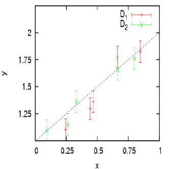
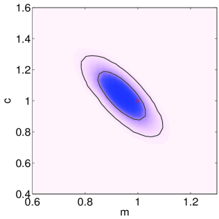
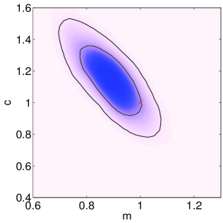
Figure 7: Upper left: Data-sets $\mathbf{D}_{1}$ and $\mathbf{D}_{2}$ drawn from a straight line model (solid line) with slope $m=1$ and intercept $c=1$ and subject to independent Gaussian noise with root mean square $\sigma_{1}=\sigma_{2}=0.1$. Upper right: Posterior $\Pr(m,c|\mathbf{D},H_{1})$ assuming that data-sets $\mathbf{D}_{1}$ and $\mathbf{D}_{2}$ are consistent. Lower left: Posterior $\Pr(m,c|\mathbf{D},H_{1})$ for data-set $\mathbf{D}_{1}$. Lower right: Posterior $\Pr(m,c|\mathbf{D},H_{1})$ for data-set $\mathbf{D}_{2}$. The inner and outer contours enclose $68$% and $95$% of the total probability respectively. The true parameter value is indicated by red crosses.

In the first case we consider $m=1$, $c=1$ and add Gaussian noise with standard deviation $\sigma_{1}=0.1$ and $\sigma_{2}=0.1$ for data-sets $\mathbf{D}_{1}$ and $\mathbf{D}_{2}$ respectively. Hence both the data-sets provide consistent information on the underlying process.

We assume that the errors $\sigma_{1}$ and $\sigma_{2}$ on the data-sets $\mathbf{D}_{1}$ and $\mathbf{D}_{2}$ are known exactly. The likelihood function can then be written as:

$$\mathcal{L}(m,c)\equiv\Pr(\mathbf{D}|m,c,H)=\prod_{i}\Pr(\mathbf{D_{i}}|m,c,H),$$ (32)

where

$$\Pr(D_{i}|m,c,H)=\frac{1}{\sqrt{2\pi\sigma_{i}^{2}}}\exp[-\chi_{i}^{2}/2]$$ (33)

and

$$\chi_{i}^{2}=\sum_{j}\frac{(y(x_{j})-\tilde{y}(x_{j}))^{2}}{\sigma_{i}^{2}}.$$ (34)

where $\tilde{y}(x_{j})$ is the predicted value of $y$ at a given $x_{j}$.

We impose uniform, $\mathcal{U}(0,2)$ priors on both $m$ and $c$. In Fig. 7 we show the data points and the posterior for the analysis assuming the data-sets $\mathbf{D}_{1}$ and $\mathbf{D}_{2}$ are consistent. The true parameter value clearly lies inside the contour enclosing $68$% of the posterior probability.

In order to quantify the consistency between the data-sets $\mathbf{D}_{1}$ and $\mathbf{D}_{2}$, we evaluate $R$ as given in Eq. 6 which for this case becomes:

$$R=\frac{\Pr(\mathbf{D}_{1},\mathbf{D}_{2}|H_{1})}{\Pr(\mathbf{D}_{1}|H_{0})\Pr(\mathbf{D}_{2}|H_{0})},$$ (35)

where the $H_{1}$ hypothesis states that the model jointly fits the data-sets $\mathbf{D}_{1}$ and $\mathbf{D}_{2}$, whereas $H_{0}$ states that $\mathbf{D}_{1}$ and $\mathbf{D}_{2}$ prefer different regions of parameter space. We evaluate,

$$\log R=3.2\pm 0.1,$$ (36)

showing strong evidence in favour of $H_{1}$.

A.1.2 Case II: Inconsistent Data-Sets

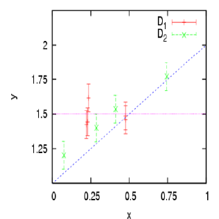
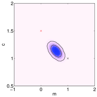
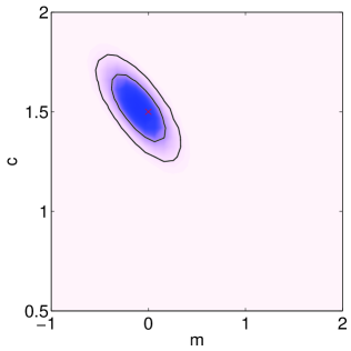
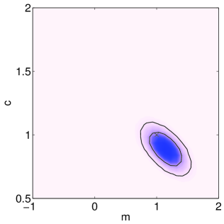
Figure 8: Upper left: Data-sets $\mathbf{D}_{1}$ and $\mathbf{D}_{2}$ drawn from a straight line model (solid line) with slope $m=0$, $c=1.5$ and $m=1$, $c=1$ respectively and subject to independent Gaussian noise with root mean square $\sigma_{1}=\sigma_{2}=0.1$. Upper right: Posterior $\Pr(m,c|\mathbf{D},H_{1})$ assuming that data-sets $\mathbf{D}_{1}$ and $\mathbf{D}_{2}$ are consistent. Lower left: Posterior $\Pr(m,c|\mathbf{D},H_{1})$ for data-set $\mathbf{D}_{1}$. Lower right: Posterior $\Pr(m,c|\mathbf{D},H_{1})$ for data-set $\mathbf{D}_{2}$. The inner and outer contours enclose $68$% and $95$% of the total probability respectively. The true parameter values are indicated by red and black crosses for Data-sets $\mathbf{D}_{1}$ and $\mathbf{D}_{2}$ respectively.

We now introduce systematic error into the data-set $\mathbf{D}_{1}$ by drawing from an incorrect straight line model with $m=0$ and $c=1.5$. Measurements for $\mathbf{D}_{2}$ are still drawn from a straight line with $m=1$ and $c=1$. We assume that the errors $\sigma_{1}=0.1$ and $\sigma_{2}=0.1$, for $\mathbf{D}_{1}$ and $\mathbf{D}_{2}$ respectively, are both quoted correctly.

We impose uniform priors, $\mathcal{U}(-1,2)$ and $\mathcal{U}(0,2)$, on $m$ and $c$ respectively. In Fig. 8 we show the data points and the posterior for the analysis assuming the data-sets $\mathbf{D}_{1}$ and $\mathbf{D}_{2}$ are consistent as well as for the analysis with data-sets $\mathbf{D}_{1}$ and $\mathbf{D}_{2}$ taken separately. In spite of the fact that the two sets of true parameter values define a direction along the natural degeneracy line in the $(m,c)$ plane, neither of the true parameter values lie inside the contour enclosing $95$% of the posterior probability. Also, it can be seen that the there is no overlap between the posteriors for data-sets $\mathbf{D}_{1}$ and $\mathbf{D}_{2}$ and so both models can be excluded at a high significance level. We again compute $R$ as given in Eq. 35 and evaluate it to be,

$$\log R=-13.1\pm 0.1,$$ (37)

showing evidence in favour of $H_{0}$ i.e. the data-sets $\mathbf{D}_{1}$ and $\mathbf{D}_{2}$ provide inconsistent information on the underlying model.

References

- [1] H. Baer and C. Balazs, analysis of the minimal supergravity model including WMAP, and constraints, JCAP 0305 (2003) 006 [arXiv:hep-ph/0303114].
- [2] J. R. Ellis, K. A. Olive, Y. Santoso and V. C. Spanos, Likelihood analysis of the CMSSM parameter space, Phys. Rev. D 69 (2004) 095004 [arXiv:hep-ph/0310356].
- [3] S. Profumo and C. E. Yaguna, A statistical analysis of supersymmetric dark matter in the MSSM after WMAP, Phys. Rev. D 70 (2004) 095004 [arXiv:hep-ph/0407036].
- [4] E. A. Baltz and P. Gondolo, Markov chain Monte Carlo exploration of minimal supergravity with implications for dark matter, JHEP 0410 (2004) 052 [arXiv:hep-ph/0407039].
- [5] J. R. Ellis, S. Heinemeyer, K. A. Olive and G. Weiglein, Indirect sensitivities to the scale of supersymmetry, JHEP 0502 (2005) 013 [arXiv:hep-ph/0411216].
- [6] L. S. Stark, P. Hafliger, A. Biland and F. Pauss, New allowed mSUGRA parameter space from variations of the trilinear scalar coupling A0, JHEP 0508 (2005) 059 [arXiv:hep-ph/0502197].
- [7] L. Alvarez-Gaume, J. Polchinski and M. B. Wise, Minimal Low-Energy Supergravity, Nucl. Phys. B 221 (1983) 495; R. Arnowitt and P. Nath, SUSY mass spectrum in SU(5) supergravity grand unification, Phys. Rev. Lett. 69, 725 (1992).
- [8] J. P. Conlon and F. Quevedo, Gaugino and scalar masses in the landscape, JHEP 0606 (2006) 029 [arXiv:hep-th/0605141]; L. E. Ibanez, The fluxed MSSM, Phys. Rev. D 71 (2005) 055005 [arXiv:hep-ph/0408064]; A. Brignole, L. E. Ibanez and C. Munoz, Towards a theory of soft terms for the supersymmetric Standard Model, Nucl. Phys. B 422 (1994) 125, Erratum-ibid. B 436 (1995) 747 [arXiv:hep-ph/9308271].
- [9] B. C. Allanach and C. G. Lester, Multi-dimensional mSUGRA likelihood maps, Phys. Rev. D 73 (2006) 015013 [arXiv:hep-ph/0507283].
- [10] L. Roszkowski, R. R. de Austri, J, Silk and R. Trotta, On prospects for dark matter indirect detection in the Constrained MSSM, [arXiv:0707.0622].
- [11] R. R. de Austri, R. Trotta and L. Roszkowski, A Markov chain Monte Carlo analysis of the CMSSM, JHEP 0605 (2006) 002 [arXiv:hep-ph/0602028].
- [12] B. C. Allanach, C. G. Lester and A. M. Weber, The dark side of mSUGRA, JHEP 12 (2006) 065 [arXiv:hep-ph/0609295]
- [13] B. C. Allanach, Naturalness priors and fits to the constrained minimal supersymmetric standard model, Phys. Lett. B 635 (2006) 123 [arXiv:hep-ph/0601089].
- [14] L. Roszkowski, R. R. de Austri and R. Trotta, Implications for the Constrained MSSM from a new prediction for , JHEP 2007 (2007) 075 [arXiv:0705.2012].
- [15] B. C. Allanach, C. G. Lester and A. M. Weber, Natural Priors, CMSSM Fits, and LHC Weather Forecasts, JHEP 08 (2007) 023 [arXiv:0705.0487].
- [16] B. C. Allanach and D. Hooper, Panglossian Prospects for Detecting Neutralino Dark Matter in Light of Natural Priors, arXiv:0806.1923 [hep-ph].
- [17] B. C. Allanach, M. J. Dolan and A. M. Weber, Global Fits of the Large Volume String Scenario to WMAP5 and Other Indirect Constraints Using Markov Chain Monte Carlo, arXiv:0806.1184 [hep-ph].
- [18] F. Feroz and M. P. Hobson, Multimodal nested sampling: an efficient and robust alternative to MCMC methods for astronomical data analysis, Mon. Not. Roy. Astron. Soc. 384 (2008) 449 [arXiv:0704.3704].
- [19] F. Feroz, M. P. Hobson and M. Bridges, MultiNest: an efficient and robust Bayesian inference tool for cosmology and particle physics, arXiv:0809.3437.
- [20] S. Heinemeyer, X. Miao, S. Su and G. Weiglein, B-Physics Observables and Electroweak Precision Data in the CMSSM, mGMSB and mAMSB, [arXiv:hep-ph/0805.2359].
- [21] C.H. Bennett, Efficient estimation of free energy differences from Monte Carlo data, Jnl. of Comp. Phys. 22 (1976) 245; A. Gelman and X.-Li Meng, Simulating normalizing constants: from importance sampling to bridge sampling to path sampling, Stat. Sci. 13 (1998) 163; R. M. Neal Estimating ratios of normalizing constants using Linked Importance Sampling, Technical Report No. 0511 (2005), Dept. of Statistics, University of Toronto
- [22] C. Gordon and R. Trotta, Bayesian calibrated significance levels applied to the spectral tilt and hemispherical asymmetry, Mon. Not. Roy. Astron. Soc. 382 (2007) 4 [arXiv:0706.3014].
- [23] R. T. Cox, Probability, frequency and reasonable expectation, Am. J. Phys. vol. 14, pp. 1-13, 1946.
- [24] J.K.O. O’Ruanaidh & W.J. Fitzgerald, 1996, Numerical Bayesian Methods Applied to Signal Processing, Springer-Verlag, New York, (1996)
- [25] M. P. Hobson, S. L. Bridle and O. Lahav, Combining cosmological data sets: hyperparameters and Bayesian evidence, Mon. Not. Roy. Astron. Soc. 335, 377 (2002) [arXiv:astro-ph/0203259].
- [26] R. Trotta, Applications of Bayesian model selection to cosmological parameters, Mon. Not. Roy. Astron. Soc. 378 (2005) 72 [arXiv:astro-ph/0504022].
- [27] B. C. Allanach and C. G. Lester, Sampling using a ‘bank’ of clues, [arXiv:hep-ph/0705.0486].
- [28] A. R. Liddle, Information criteria for astrophysical model selection, Mon. Not. Roy. Astron. Soc. 377 (2007) [arXiv:astro-ph/0701113].
- [29] J. Skilling, AIP Conference Proceedings of the 24th International Workshop on Bayesian Inference and Maximum Entropy Methods in Science and Engineering, Vol. 735, pp. 395-405 (2004) available from http://www.inference.phy.cam.ac.uk/bayesys/
- [30] R. Trotta, Bayes in the sky: Bayesian inference and model selection in cosmology, Invited review, Contemporary Physics, Vol. 49, No. 2, March-April (2008) [arXiv:0803.4089].
- [31] R. D. Cousins, Comment on “Bayesian Analysis of Pentaquark Signals from CLAS Data”, with Response to the Reply by Ireland and Protopopsecu [arXiv:0807.1330 [hep-ph]].
- [32] P. Marshall, N. Rajguru and A. Slosar, Bayesian evidence as tool for comparing datasets, Phys. Rev. D73 (2006) 067302
- [33] W. -M. Yao et al. [Particle Data Group], J. Phys. G33 (2006) 1. and 2007 partial update for 2008.
- [34] The Tevatron Electroweak Working Group, Combination of CDF and D0 results on the mass of the top quark, hep-ex/0703034
- [35] The Tevatron Electroweak Working Group, Combination of CDF and D0 Results on the Mass of the Top Quark, arXiv:0808.1089 [hep-ex].
- [36] J. P. Miller, E. de Rafael and B. L. Roberts, Rept. Prog. Phys. 70 (2007) 795.
- [37] Precision Electroweak Measurements and Constraints on the Standard Model, The LEP Collaboration, [arXiv:0712.0929]
- [38] The code is forthcoming in a publication by A. M. Weber et al.; S. Heinemeyer, W. Hollik, D. Stöckinger, A. M. Weber and G. Weiglein, Precise prediction for M(W) in the MSSM, JHEP 08 (2006) 052, [arXiv:hep-ph/0604147].
- [39] [The ALEPH, DELPHI, L3 and OPAL Collaborations, the LEP Electroweak Working Group], Precision Electroweak Measurements and Constraints on the Standard Model, [arXiv:hep-ph/0712.0929].
- [40] F. Mahmoudi SuperIso: A program for calculating the isospin asymmetry of in the MSSM, Computer Physics Communications (2008), [arXiv:0710.2067].
- [41] F. Mahmoudi New constraints on supersymmetric models from , JHEP 12 (2007) 026, [arXiv:0710.3791].
- [42] available at http://www.slac.stanford.edu/xorg/hfag/rare/leppho07/radll/index.html
- [43] UTfit Collaboration, The Unitarity Triangle Fit in the Standard Model and Hadronic Parameters from Lattice QCD: A Reappraisal after the Measurements of and , JHEP (2006), [arXiv:hep-ph/0606167].
- [44] B. C. Allanach, SOFTSUSY: A program for calculating supersymmetric spectra, Comput. Phys. Commun. 143 (2002) 305, [arXiv:hep-ph/0104145].
- [45] P. Skands et al., SUSY Les Houches accord: Interfacing SUSY spectrum calculators, decay packages, and event generators, JHEP 0407 (2004) 036, [arXiv:hep-ph/0311123].
- [46] G. Bélanger, F. Boudjema, A. Pukhov and A. Semenov, micrOMEGAs: Version 1.3, Comput. Phys. Commun. 174 (2006) 577, [arXiv:hep-ph/0405253]; G. Bélanger, F. Boudjema, A. Pukhov and A. Semenov, micrOMEGAs: A program for calculating the relic density in the MSSM, Comput. Phys. Commun. 149 (2002) 103, [arXiv:hep-ph/0112278].
- [47] G.W. Bennett et al. [Muon g-2 collaboration], Final report of the muon E821 anomalous magnetic moment measurement at BNL, Phys. Rev. D 73 (2006) 072003 [arXiv:hep-ex/0602035].
- [48] M. Passera, Precise mass-dependent QED contributions to leptonic g-2 at order alpha**2 and alpha**3, Phys. Rev. D 75 (2007) 013002, [arXiv:hep-ph/0606174].
- [49] A. Czarnecki, W.J. Marciano, and A. Vainshtein, Refinements in electroweak contributions to the muon anomalous magnetic moment, Phys. Rev. D 67 (2003) 073006, [arXiv:hep-ph/0212229]
- [50] U. Chattopadhyay and P. Nath, Probing supergravity grand unification in the Brookhaven g-2 experiment, Phys. Rev. D 53 (1996) 1648, [arXiv:hep-ph/9507386].
- [51] S. Heinemeyer, D. Stöckinger and G. Weiglein, Electroweak and supersymmetric two-loop corrections to (g-2)(mu), Nucl. Phys. B690 (2004) 103, [arXiv:hep-ph/0405255]; S. Heinemeyer, D. Stöckinger and G. Weiglein, Two-loop SUSY corrections to the anomalous magnetic moment of the muon, Nucl. Phys. B 690 (2004) 62, [arXiv:hep-ph/0312264].
- [52] D. Stöckinger, The muon magnetic moment and supersymmetry, J.Phys. G34 (2007) R45-R92 [arXiv:hep-ph/0609168].
- [53] M. Awramik, M. Czakon, A. Freitas, and G. Weiglein, Precise prediction for the W-boson mass in the standard model, Phys. Rev. D 69 (2004) 053006 [arXiv:hep-ph/0311148].
- [54] J. Haestier, S. Heinemeyer, D. Stöckinger and G. Weiglein, Electroweak precision observables: Two-loop Yukawa corrections of supersymmetric particles, JHEP 0512 (2005) 027, [arXiv:hep-ph/0508139].
- [55] E. Barberio et al [Heavy Flavour Averaging Group], Averages of b-hadron Properties at the End of 2005, arXiv:hep-ex/0603003.
- [56] M. Misiak and M. Steinhauser, NNLO QCD corrections to the matrix elements using interpolation in , Nucl. Phys. B764 (2007) 62, [arXiv:hep-ph/0609241].
- [57] M. Misiak et al., Estimate of at , Phys. Rev. Lett. 98 (2005) 022002 [arXiv:hep-ph/0609232].
- [58] C.S. Lin, private communication.
- [59] G. Isidori and P. Paradisi, Hints of large tan(beta) in flavour physics, Phys. Lett. B 639, 499 (2006) [arXiv:hep-ph/0605012].
- [60] A. J. Buras, P. H. Chankowski, J. Rosiek and L. Slawianowska, Delta(M(d,s)), B/(d,s)0 mu+ mu- and B X/s gamma in supersymmetry at large tan(beta), Nucl. Phys. B 659 (2003) 3 [arXiv:hep-ph/0210145].
- [61] E. Komatsu et al., Five Year Wilkinson Microwave Anisotropy Probe (WMAP) Obsercations: Cosmological Interpretation, [arXiv:0803.0547].
- [62] A. Arbey and F. Mahmoudi, SUSY constraints from relic density: high sensitivity to pre-BBN expansion rate, [arXiv:0803.0741].
- [63] V. Barger, D. Marfatia, A. Mustafayev, Neutrino sector impacts SUSY dark matter, [arXiv:hep-ph/0804.3601].
- [64] N. Baro, F. Boudjema and A. Semenov, Full one-loop corrections to the relic density in the MSSM: A few examples, Phys. Lett. B 660 (2008) 550, [arXiv:hep-ph/0710.1821.
- [65] K. L. Chan, U. Chattopadhyay and P. Nath, Naturalness, weak scale supersymmetry and the prospect for the observation of supersymmetry at the Tevatron and at the LHC, Phys. Rev. D 58, 096004 (1998) [arXiv:hep-ph/9710473].
- [66] D. Feldman, Z. Liu and P. Nath, Light Higgses at the Tevatron and at the LHC and Observable Dark Matter in SUGRA and D Branes, Phys. Lett. B 662, 190 (2008) [arXiv:0711.4591 [hep-ph]].
- [67] J. R. Ellis, S. Heinemeyer, K. A. Olive and G. Weiglein, Phenomenological indications of the scale of supersymmetry, JHEP 0605 (2006) 005, [arXiv:hep-ph/0602220].
- [68] B. C. Allanach, J. P. J. Hetherington, M. A. Parker and B. R. Webber, JHEP 0008 (2000) 017 [arXiv:hep-ph/0005186].
- [69] M. P. Hobson and C. McLachlan, A Bayesian approach to discrete object detection in astronomical datasets, Mon. Not. Roy. Astron. Soc. 338 (2003) 765 [astro-ph/0204457].
- [70] P. J. Marshall, M. P. Hobson, A. Slosar, Bayesian joint analysis of cluster weak lensing and Sunyaev-Zel’dovich effect data, Mon. Not. Roy. Astron. Soc. 346 (2003) 489 [astro-ph/0307098]
- [71] A. Slosar et al., Cosmological parameter estimation and Bayesian model comparison using VSA data, Mon. Not. Roy. Astron. Soc., 341 (2003) L29 [astro-ph/0212497]
- [72] P. Mukherjee, D. Parkinson, A. R. Liddle, A nested sampling algorithm for Bayesian model selection, Astrophys. J., 638 (2006) L51 [astro-ph/0508461].
- [73] B. A. Basset, P. S. Corasaniti, M. Kunz, The essence of quintessence and the cost of compression, Astrophys. J., 617 (2004) L1 [astro-ph/0407364].
- [74] R. Trotta, Application of Bayesian model selection to cosmological parameters, Mon. Not. Roy. Astron. Soc., 378 (2007) 72 [astro-ph/0504022].
- [75] M. Beltran, J. Garcia-Bellido, J. Lesgourgues, A. Liddle, A. Slosar, Bayesian model selection and isocurvature perturbations, Phys. Rev. D, 71 (2005) 063532 [astro-ph/0501477].
- [76] M. Bridges, A. N. Lasenby, M. P. Hobson, A Bayesian analysis of the primordial power spectrum, Mon. Not. Roy. Astron. Soc. 369 (2006) 1123 [astro-ph/0511573].
- [77] R. Trotta, The isocurvature fraction after WMAP 3-years data, Mon. Not. Roy. Astron. Soc. 375, L26-L30 (2007) [arXiv:astro-ph/0608116].