Dynamical transition, hydrophobic interface, and the temperature dependence of electrostatic fluctuations in proteins

Abstract

Molecular dynamics simulations have revealed a dramatic increase, with increasing temperature, of the amplitude of electrostatic fluctuations caused by water at the active site of metalloprotein plastocyanin. The increased breadth of electrostatic fluctuations, expressed in terms of the reorganization energy of changing the redox state of the protein, is related to the formation of the hydrophobic protein/water interface allowing large-amplitude collective fluctuations of the water density in the protein’s first solvation shell. On the top of the monotonic increase of the reorganization energy with increasing temperature, we have observed a spike at 220 K also accompanied by a significant slowing of the exponential collective Stokes shift dynamics. In contrast to the local density fluctuations of the hydration-shell waters, these spikes might be related to the global property of the water solvent crossing the Widom line.

I Introduction

Dynamical transition has been observed in many hydrated biopolymers, including proteins, DNA, and RNA Rasmussen et al. (1992); Lee and Wand (2001); Parak (2003); Caliskan et al. (2006). In amounts to a sharp change in the temperature slope of mean-squared atomic displacements of the biopolymer atoms at the temperature usually observed in the range $T_{\text{tr}}=200-230$ K. While the microscopic origin of this dynamical transition is still debated Chen et al. (2006a); Kumar et al. (2006); Pawlus et al. (2008); Khodadadi et al. (2008); Ngai et al. (2008), an important open question is how the existence of this universal property of hydrated biopolymers Ringe and Petsko (2003) affects their physiological activity Parak et al. (1980); Rasmussen et al. (1992); Lee and Wand (2001); Ringe and Petsko (2003).

Electrostatics is significant to the catalytic action of enzymes Warshel and Parson (2001). Therefore, a link between protein’s dynamical transition and enzymatic activity may exist in some property characterizing electrostatics at the active site. It is currently well established that the dynamical transition is not observed in dry proteins, and its existence is universally attributed to the interaction of water with the protein interface. A property sensitive to the dynamical transition needs to connect water’s electrostatics to protein’s active site. Here, we consider one such parameter which critically affects barriers of protein redox reactions, the reorganization energy of electron transfer Marcus and Sutin (1985).

The reorganization energy $\lambda$ of electronic transitions between proteins characterizes the breadth of thermal fluctuations of the energy gap $\Delta E$ between the donor and acceptor energy levels

$$\lambda=\beta\langle\left(\delta\Delta E\right)^{2}\rangle/2.$$ (1)

Here, $\delta\Delta E$ is the fluctuation of the energy gap $\Delta E$ and the inverse temperature $\beta=1/(k_{\text{B}}T)$ corrects for the proportionality of the variance to temperature following from the fluctuation-dissipation theorem Landau and Lifshits (1980). The reorganization energy $\lambda$ is then typically a weak function of temperature when measured for electronic transitions in molecular polar solvents Matyushov (2007).

Experimentally accessible reorganization energy of interprotein electron transfer Gray and Winkler (2005) characterizes the coupling of the energy levels of both the donor and acceptor to the thermal bath. For long-distance electron transfer, most common in biological energy chains, $\lambda$ can be split into a sum of individual, donor and acceptor, components and a Coulomb correction. Since these individual components mostly characterize the physics of the problem, our focus here is on the electrostatic fluctuations at the active site of a single protein.

Electron transfer changes the redox state of the protein and thus the partial atomic charges of the active site. The electrostatic interactions of these charge differences with the potential of the hydrating water $\phi_{w,j}$ at atomic sites $j$ contribute to the Coulomb shift $\Delta E_{w}^{C}$ which is a part of the overall donor-acceptor energy gap:

$$\Delta E_{w}^{C}=\sum_{j}\Delta q_{j}\phi_{w,j}.$$ (2)

Here, the sum runs over the atoms of the active site. The variance of this Coulomb energy gap calculated for the charges $\Delta q_{j}$ of the active site of a single protein is what is studied in this paper. The water reorganization energy is then defined as

$$\lambda_{w}=\beta\langle(\delta\Delta E_{w}^{C})^{2}\rangle/2.$$ (3)

The dynamical dimension of the problem is characterized by the normalized Stokes shift correlation function Jimenez et al. (1994)

$$S_{w}(t)=\langle\delta\Delta E_{w}^{C}(t)\delta\Delta E_{w}^{C}(0)\rangle/\langle(\delta\Delta E_{w}^{C}(0))^{2}\rangle,$$ (4)

where angular brackets denote an ensemble average. The common form of $S_{w}(t)$ is dense polar liquids includes a fast one-particle component with a Gaussian decay followed by exponential (or stretched exponential) decay describing collective solvent dynamics Jimenez et al. (1994)

$$S_{w}(t)=A_{G}e^{-(t/\tau_{G})^{2}}+(1-A_{G})e^{-(t/\tau_{E})^{\beta_{E}}}.$$ (5)

Here, $\tau_{G}$ and $\tau_{E}$ are, respectively, the Gaussian and exponential relaxation times and $A_{G}$ quantifies the relative weight of single-particle dynamics in the reorganization energy; $\beta_{E}$ is the stretching exponent.

The main result of the Molecular Dynamics (MD) simulations presented here is to show that the reorganization energy $\lambda_{w}(T)$ rises significantly with temperature to a value much exceeding both the common estimates of this parameter for reactions involving small redox molecules,Marcus and Sutin (1985) and previous estimates for protein electron transfer Warshel and Parson (2001). We associate this increase with the formation of the hydrophobic interface allowing large-amplitude fluctuations of the local water density. We also show that both the long-time exponential relaxation time [$\tau_{E}$ in Eq. (5)] and the collective part of the reorganization energy $\lambda_{E}=(1-A_{G})\lambda_{w}$ pass through peaks at the temperature of dynamical transition $T_{\text{tr}}=220$ K. This special temperature (at atmospheric pressure) has been previously associated with a thermodynamic singularity in the phase diagram of bulk water Xu et al. (2005); Angell (2008). It has also been recently suggested that a transition from fragile to strong dynamics of hydrated biopolymers occurs at the same temperature Chen et al. (2006a, b); Lagi et al. (2008).

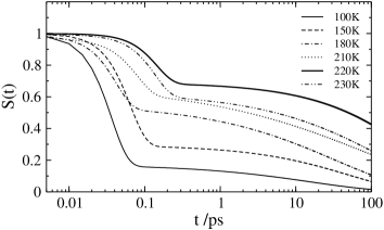
Figure 1: Stokes shift correlation function of PC (Ox) at different temperatures indicated in the plot

II MD Simulations

MD simulations reported here have been done for the redox metalloprotein plastocyanin (PC) from spinach according to the simulation protocol described in our previous publication LeBard and Matyushov (2008a). PC is a single polypeptide chain of 99 residues forming a $\beta$-sandwich, with a single copper ion ligated by cysteine, methionine, and two histidines. The protein’s active site in our analysis is composed of a copper ion and four atoms (two nitrogens and two sulfurs) coordinating it. The partial charges on these atoms in both reduced (Red) and oxidized (Ox) states can be found in Ref. LeBard and Matyushov, 2008b.

The initial configuration of PC was taken from a protonated X-ray crystal structure with a 1.7 Å resolution (PDB: 1ag6, Xue et al. (1998)). First, the initial protein configuration was minimized in vacuum using the conjugate gradient method for 10⁴ steps to remove any bad contacts. Then, the system was solvated in an octahedral box with $N_{w}=5886$ TIP3P molecules Jorgensen et al. (1983), providing at least two solvation shells around the protein. The protein was simulated in the Ox state with a total charge of $-8$ and in the Red state with the total charge of $-9$. In both cases, eight or nine sodium ions were added to neutralize the system, as is required for the Ewald summation. After adding the water and counterions, the system’s energy was minimized for another $10^{4}$ steps while the protein was allowed to relax and the water and sodium atoms were positionally constrained. Finally, the entire system was additionally minimized for $10^{5}$ steps.

Following minimization, the system was heated in a $NVT$ ensemble for 30 ps from 0 K to the desired temperature. Temperature equilibration was followed by a 2 ns density equilibration in a $NPT$ ensemble at $P=1$ atm. This equilibrated structure was then used for 20 individual simulations of the Ox state and 7 simulations of the Red state of PC to create 10 ns long trajectories. Temperatures $T$ was varied from 100 to 300 K at constant volume $V$ and constant number of water molecules $N_{w}$. The total simulation time was 324 ns and required 6.9 CPU years, while only 270 ns were used for the production data analysis which lasted another 2.2 CPU years. The timestep for all MD simulations was 2 fs, and SHAKE was used to constrain bonds to hydrogen atoms. Constant temperature and pressure simulations employed Berendsen thermostat and barostat, respectively Berendsen et al. (1984). The long-range electrostatics were calculated using a smooth particle mesh Ewald summation with a $9$ Å limit in the direct space sum.

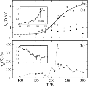
Figure 2: Panel (a): Points are the water reorganization energies $\lambda_{w}$ from MD simulations of PC (Ox) and the solid line shows the fit of the simulation data to Eq. (7) with the fitting parameters: $\lambda_{G}=0.39$ eV, $\lambda_{\text{eq}}=0.87+0.0084*T$ eV, $\tau_{\text{obs}}/\tau_{0}=7350$, and $E_{a}=1867$ K; the dashed line assumes temperature-independent $\lambda_{\text{eq}}$. The inset shows the exponential part of the reorganization energy related to collective water fluctuations. The closed diamonds refer to half of the Stokes shift [Eq. (8)] and the open diamonds show the linear-response reorganization energy $\lambda_{w}^{\text{Ox}}$ obtained from Eq. (9). Panel (b): The points refer to the exponential relaxation time of the Stokes shift correlation function obtained from MD of PC(Ox) and the inset shows the Gaussian amplitude $A_{G}$ in Eq. (5).

III Results

Most MD results reported here have been obtained from configurations in equilibrium with the Ox state of PC; the Stokes shift data were collected from both Ox and Red equilibrium trajectories as discussed below. The reorganization energies $\lambda_{w}(T)$ of PC(Ox) state were obtained from MD trajectories at different temperatures $T$ and fixed observation window $\tau_{\text{obs}}=1$ ns. More specifically, the reorganization energy is calculated from the variance of the Coulomb energy gap [Eq. (1)] by sliding a 1 ns observation window along a longer MD trajectory and averaging over the results of the variance calculations on each window. The average $\langle\Delta E_{w}^{C}\rangle_{\text{obs}}$ required to calculate the variance is not a global average but is obtained separately from each observation window. This approach to the calculation of averages is analogous to a laboratory procedure with a fixed resolution and is required for studies of systems with broad distributions of relaxation times LeBard and Matyushov (2008a). In case of proteins, a subset of nuclear motions is always frozen on the simulation time-scale and so both specifying the observation window and keeping it constant for all measurements is significant in maintaining consistent conditions for collecting the data.

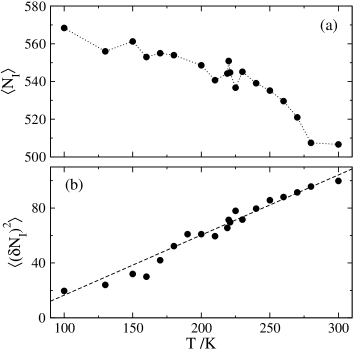
Figure 3: Average number of water molecules in PC’s first solvation shell (a) and its variance (b) vs temperature. The dashed line in (b) shows a linear regression through the points and the dotted line in (a) connects the simulation points.

Fits of the simulated Stokes shift functions to Eq. (5) are shown in Fig. 1. Two features are most prominent there: the increase of the relative importance of the collective solvent dynamics with increasing temperature (decrease of $A_{G}$ in Eq. (5)), and the appearance of a peak in the exponential relaxation time at $T_{\text{tr}}=220$ K (Fig. 2b). The exponential part of the reorganization energy $\lambda_{E}$ also shows a peak at the same temperature (inset in Fig. 2a).

Table 1: Properties of hydrated plastocyanin (Ox) from MD simulations.

$T$/K	$\lambda_{w}$	$\langle N_{I}\rangle$	$\langle(\delta N_{I})^{2}\rangle$	$p_{2}$	$D$	$\tau_{E}$
100	0.15	568	20	$-0.015$	0.032	15.5
130	0.50	556	24	$-0.022$	0.003	52.0
150	0.32	561	32	$-0.025$	0.017	48.6
160	0.63	553	30	$-0.021$	0.015	54.3
170	0.75	555	42	$-0.030$	0.038	57.8
180	0.52	554	52	$-0.025$	0.041	32.0
190	0.95	552	61	$-0.025$	0.020	15.9
200	1.08	549	61	$-0.027$	0.037	125.5
210	1.33	541	60	$-0.027$	0.061	84.9
219	1.79	544	66	$-0.025$	0.088	409.6
220	2.15	537	71	$-0.021$	0.093	353.6
221	1.90	545	70	$-0.025$	0.095	166.5
225	2.02	537	78	$-0.021$	0.107	104.8
230	2.12	545	72	$-0.021$	0.126	157.8
240	2.07	539	80	$-0.020$	0.165	127.0
250	2.97	535	86	$-0.020$	0.206	147.8
260	2.71	530	88	$-0.018$	0.281	102.1
270	2.57	520	91	$-0.016$	0.326	68.5
280	3.05	507	96	$-0.012$	0.389	93.8
300	3.33	507	100	$-0.014$	0.536	68.1

Overall $\lambda_{w}(T)$ strongly increases from a value typical for short MD simulations of proteins Warshel and Parson (2001) to a much larger value at higher temperatures (Fig. 2a and Table 1). The temperature of the onset of the $\lambda_{w}(T)$ rise is much below $T_{\text{tr}}$, at about 150 K commonly associated with the onset of rotation of methyl groups of protein’s side chains Khodadadi et al. (2008); Krishnan et al. (2008). This onset temperature is however depends on the observation window. Since the relaxation times of the protein are widely different, the rise of $\lambda_{w}(T)$ is caused by the appearance of a particular relaxation mode in the observation window, methyl rotations in this case. However, we believe that the underlying picture is more complex and the main rise of $\lambda_{w}(T)$ is caused not by methyl rotations, but by a more collective mode coupled to the solvent interfacial translations Vitkup et al. (2000); Tarek and Tobias (2002) (see below). In fact recent extensive simulations of the mean-squared atomic displacements of myoglobin Krishnan et al. (2008) have reveled two breaks in the temperature slope: the first break at 150 K related to methyl (anharmonic) rotations followed by a stronger solvent-induced break at 220 K.

The appearance of a relaxation mode in the observation window restores the statistical ergodicity for that particular mode. The non-ergodic rise of $\lambda_{w}(T)$ to its equilibrium value $\lambda_{\text{eq}}(T)$, also seen for model charge-transfer chromophores Ghorai and Matyushov (2006), can be described by imposing a step-wise frequency filter on the spectrum of Stokes shift fluctuations Matyushov (2007)

$$\lambda_{w}(T)=2\lambda_{\text{eq}}(T)\int_{1/\tau_{\text{obs}}}^{\infty}S_{w}(\omega)d\omega.$$ (6)

Here, $S_{w}(\omega)$ is the Fourier transform of the Stokes shift correlation function in Eqs. (4) and (5). In order to provide a physically transparent form for $\lambda_{w}(T)$ one can consider an effective single-exponential Debye relaxation, instead of several relaxation modes, to characterize collective nuclear motions coupled to the Stokes shift dynamics. This procedure leads to the following simple relation

$$\lambda_{w}(T)=\lambda_{G}+(\lambda_{\text{eq}}(T)-\lambda_{G})(2/\pi)\mathrm{arctg}\left[\tau_{\text{obs}}/\tau(T)\right],$$ (7)

where the effective Debye relaxation time is given by the Arrhenius law, $\tau(T)=\tau_{0}\exp[\beta E_{a}]$.

The Gaussian component of the solvent reorganization energy, related to ballistic water motions Jimenez et al. (1994), is normally reasonably temperature-independent Ghorai and Matyushov (2006). On the other hand, the temperature decrease of $A_{G}(T)\simeq\lambda_{G}/\lambda_{\text{eq}}(T)$ in the fit of the Stokes shift function (inset in Fig. 2b) clearly points to the equilibrium reorganization energy increasing with temperature. From the anticipated relation of $\lambda_{\text{eq}}(T)$ with the variance of the number of particles in the first solvation shell, which linearly grows with temperature (see below), we have attempted a linear temperature dependence of $\lambda_{\text{eq}}(T)$ to fit the MD data to Eq. (7). The result is shown by the solid line in Fig. 2a, and it is not much different from the fit using a temperature-independent $\lambda_{\text{eq}}$ (dashed line in Fig. 2a). We also note that since our simulation length obviously cuts some slow nuclear modes off, we have not used $A_{G}(T)$ from the fits of the Stokes shift correlation functions to calculate $\lambda_{\text{eq}}(T)$.

The activation energy $E_{a}$ of the effective Debye mode obtained from the fit, $E_{a}=1867$ K, points to a secondary $\beta$-relaxation mode creating fluctuations of the electrostatic potential, in contrast to the primary $\alpha$-relaxation of the water/protein system with a commonly much higher activation barrier Green et al. (1994); Fenimore et al. (2004). This activation energy is also lower than $\beta$ relaxation of aqueous mixtures with the activation energy of the order of $5.5\times 10^{3}$ K Ngai et al. (2008).

Also shown in Fig. 2a (closed diamonds) is the reorganization energy from the Stokes shift obtained from the difference of average Coulomb energy gaps in Ox and Red states:

$$\lambda_{w}^{\text{St}}=\frac{1}{2}\left|\langle\Delta E_{w}^{C}\rangle_{\text{Ox}}-\langle\Delta E_{w}^{C}\rangle_{\text{Red}}\right|$$ (8)

For water fluctuations following linear response one expects the reorganization energy from the variance [Eq. (3)] to be connected to the reorganization energy from the two first moments [Eq. (8)] by the following relation:

$$\lambda_{w}^{\text{Ox}}=\lambda_{w}^{\text{St}}-(\beta/2)\langle\delta\Delta E_{w}^{C}\delta\Delta E_{P}^{C}\rangle_{\text{Ox}}.$$ (9)

In Eq. (9) we have stressed that the averages are taken over the configurations in equilibrium with PC(Ox) and $\Delta E_{P}^{C}$ is the Coulomb interaction energy of the difference charges of the active site [$\Delta q_{j}$, Eq. (2)] with the remaining partial charges of the protein matrix.

When a rigid molecule is solvated and the intramolecular energy gap does not fluctuate, the second correlator in Eq. (9) is zero. One arrives then at the standard expectation of the linear solvation theories that two routes to the reorganization energy, from the second cumulant [Eq. (3)] and from two first cumulants [Eq. (8)], are equivalent Marcus and Sutin (1985); Matyushov (2007). Since the protein matrix fluctuates itself, the cross-correlation in principle needs be taken into account, and it turns out to be negative Nilsson and Halle (2005). However, when cross-correlation term is subtracted from $\lambda_{w}^{\text{St}}$ in Eq. (9) (open diamonds in Fig. 2a), the result is still significantly below the reorganization energy from the variance [Eq. (3)]. We therefore observe here a severe breakdown of linear solvation.

What Fig. 2a in fact indicates is that the two definitions of the reorganization energy converge at low temperatures with the reorganization energy from the variance deviating significantly upward above $T\simeq 200$ K. This observation implies that fast water’s modes coupled to electrostatic fluctuations, presumably librations, which are still unfrozen at low temperatures, follow the expectations of the linear response theories. On the contrary, a slower collective mode, which appears in the observation window at higher temperatures and gives rise to the gigantic reorganization energy, does not follow the linear response. The cross-correlation does not restore the linear response, in contrast to an earlier observation made for a water-exposed tryptophan residue Nilsson and Halle (2005). The low value of the cross-correlation physically implies that the elasticities of the protein and water are drastically different and their electrostatic fluctuations are mostly decoupled. From that perspective, this correlation decoupling should hold for any solute/solvent combination with a significantly different rigidity.

The fluctuations of water’s electrostatic potential at the active site can generally be traced back to two weakly correlated nuclear modes in polar liquids, the orientational polarization and the local density Matyushov (1993). In order to clarify the origin of the dramatic rise of the reorganization energy, we have looked at two additional correlation functions characterizing the density and orientational manifolds of the water molecules in the protein’s first solvation shell. A water molecule is defined as to belong to the first solvation shell if its oxygen atom is within 2.87 Å distance from the protein van der Waals surface.

The density manifold is characterized by the fluctuation of the number of particles $N_{I}(t)$ in the first solvation shell,

$$C_{N}(t)=\langle\delta N_{I}(t)\delta N_{I}(0)\rangle.$$ (10)

Further, the orientational manifold is described by the fluctuations of the total dipole moment $\mathbf{M}(t)$ of the water dipoles in the first solvation shell,

$$C_{M}(t)=\langle N_{I}\rangle^{-1}\langle\delta\mathbf{M}(t)\cdot\delta\mathbf{M}(0)\rangle,$$ (11)

where $N_{I}(T)=\langle N_{I}\rangle$ is the average number of waters in the first solvation shell. In $C_{N}(t)$ and $C_{M}(t)$, the fluctuations $\delta N_{I}(t)$ and $\delta\mathbf{M}(t)$ denote the deviations from the corresponding average values. The variances were calculated on the 1 ns observation window by using the same procedure as for the reorganization energy calculations.

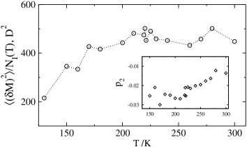
Figure 4: $\langle(\delta M)^{2}\rangle/N_{I}(T)$ vs temperature. The inset shows the second-rank orientational order parameter $p_{2}(T)$ [Eq. (12)].

The temperature dependences of the average and variance of the number of waters in the first solvation shell (Fig. 3) are indicative of the formation of the hydrophobic protein/water interface with increasing temperature. The average $N_{I}(T)$ is generally a decaying function (Fig. 3a), and the slope of this decay becomes sharper above the transition temperature $T_{\text{tr}}$ (see below). The decrease in the density of water at the interface allows stronger density fluctuations (Fig. 3b) and it is this regime of large interfacial density fluctuations that is a signature of hydrophobic solvation Chandler (2005). In this regime, one-particle exchanges of water molecules between the surface and the bulk Tarek and Tobias (2002) combine into large-scale collective density waves producing significant modulations of the electrostatic potential reflected in $\lambda_{w}(T)$. This thermal noise of hydrophobic surfaces is also reflected in a well-documented increase of protein’s heat capacity upon unfolding, indicative of an increased breadth of the energy fluctuations Huang and Chandler (2000); Prabhu and Sharp (2005).

The interfacial density fluctuations originate from the exchange of waters between the hydration shell and the bulk. These fluctuations can be represented as binding/unbinding events at the protein surface Matyushov (2008) with the resulting equilibrium reorganization energy $\lambda_{\text{eq}}(T)$ scaling linearly with the variance of the number of particles in the hydration shell: $\lambda_{w}(T)=a+b\langle(\delta N_{I})^{2}(T)\rangle$, where coefficients $a$ and $b$ are weak functions of temperature. This expectation, used in the solid-line fit in Fig. 2a, is corroborated quite well given the linear scaling of $\langle(\delta N_{I})^{2}(T)\rangle$ with temperature (Fig. 3b). A fairly significant temperature rise of $\lambda_{\text{eq}}(T)$ (see the fitting parameters in Fig. 2) also indicates a substantial density component in the overall reorganization energy at ambient conditions, in contrast to a 20–30% contribution for small solutes in dense polar solvents Matyushov (1993). We therefore conclude that the contribution to $\lambda_{\text{eq}}(T)$ from density fluctuations is significantly magnified by the soft and flexible nature of the hydrophobic protein/water interface resulting in a gigantic magnitude of the overall reorganization energy far exceeding half of the Stokes shift [Eqs. (8) and (9)].

The orientational fluctuations of the first-shell dipoles do not show a resolvable correlation with the reorganization energy (Fig. 4). The variance of the first-shell dipole moment grows with rising temperature, in accord with a general expectation of increased softness of the solvation shell, but does not show an obvious correlation with $\lambda_{w}(T)$. There is a weak maximum at $T_{\text{tr}}$ for $\langle(\delta\mathbf{M})^{2}\rangle$, but it is hard to assess from our data whether this is another reflection of the same spike seen for the collective part of the reorganization energy $\lambda_{E}$ in Fig. 2a.

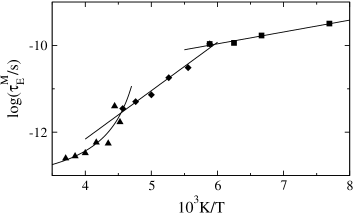
Figure 5: Exponential relaxation time $\tau_{E}^{M}$ extracted by fitting the correlation function $C_{M}(t)$ from Eq. (11) to Eq. (5). The points are the simulation results in three ranges of temperature where they are fitted to the Vogel-Fulcher temperature law (at highest temperatures) and to Arrhenius laws (at intermediate and lowest temperature ranges). The solid lines show the results of the fits.

The inset in Fig. 4 shows the second-rank orientational order parameter

$$p_{2}=\left\langle\sum_{j\in I}P_{2}(\mathbf{\hat{e}}_{j}\cdot\mathbf{\hat{r}}_{j})\right\rangle.$$ (12)

Here, $\mathbf{\hat{e}}_{j}$ and $\mathbf{\hat{r}}_{j}$ are the unit vectors of the dipole moment and position of molecule $j$ which belongs to the first solvation shell, and $P_{2}(x)$ is the second Legendre polynomial. The low-temperature portion of $p_{2}(T)$ is practically constant showing a slight preferential orientation of the water molecules parallel to the interface. This type of ordering has been previously observed at interfaces of nonpolar substances and proteins with water Lee et al. (1984); Gerstein and Lynden-Bell (1993). This preferential ordering decays with increasing temperature resulting in essentially random, on average, orientations of water dipoles in the hydration shell. The fairly large amplitude of the dipole moment fluctuations is therefore most likely caused by the density fluctuations.

This assessment is supported by the data for exponential relaxation times of $C_{N}(t)$ and $C_{M}(t)$ obtained by fitting these correlation functions to Eq. (5). When both exponential relaxation times are fitted to Arrhenius laws, they produce activation energies of 1389 K and 2076 K, respectively, in a close range with the activation energy of 1867 K obtained from the fit of $\lambda_{w}(T)$ to Eq. (7). We note that this activation barrier is consistent with the activation enthalpies of 1400–2400 K obtained by a variety of techniques for $\beta$-fluctuations of hydrated proteins Fenimore et al. (2004) which are considered to be slaved by $\beta$-fluctuations of the hydration shell Fenimore et al. (2004); Swenson et al. (2007). One also needs to keep in mind that an average Arrhenius slope actually hides a fairly complex behavior. Figure 5 shows the exponential relaxation time of $C_{M}(t)$ vs inverse temperature. The low-temperature portion of the data (triangles) is well approximated by a non-Arrhenius Vogel-Fulcher temperature law. This is followed by what can be characterized as a fragile-to-strong crossover followed by yet another break in the Arrhenius slope at $\simeq 160$ K. This picture is consistent with two breaks in the slope seen in the simulations of mean-squared atomic displacements of myoglobin Krishnan et al. (2008), where the lowest-temperature break was associated with the onset of methyl group rotations. The results for exponential relaxation times of $C_{N}(t)$ are more scattered and we could not reach an equally informative conclusion except for the average Arrhenius slope.

IV Discussion

Many alternative explanations have been sought for the observed dynamical transition in biopolymers Ringe and Petsko (2003). Given that the transition is not observed for dry protein samples, the possible scenarios are limited to either the protein/water interface or to a bulk property of water. The recent observations, from neutron scattering measurements, of the fragile-to-strong crossover in the dynamics of partially hydrated protein powder samples Chen et al. (2006a) point to the second (bulk water) scenario. The crossover, also seen in the recent simulations Kumar et al. (2006); Lagi et al. (2008), can be connected to the bulk water crossing the Widom line, i.e. the line of maximum cooperativity of the water fluctuations Xu et al. (2005). On the other hand, other recent experimental data on quasielsatic neutron scattering, dielectric relaxation Khodadadi et al. (2008), and conductivity Pawlus et al. (2008) of hydrated proteins have not revealed any special points in the corresponding relaxation times around the temperature of dynamical transition. These latter data report the temperature dependence of the primary $\alpha$-relaxation of the protein/water system and therefore these authors have concluded that the observed dynamical crossover Chen et al. (2006a) should be attributed the appearance of a secondary relaxation in the observation window at $T>T_{\text{tr}}$ Swenson et al. (2007); Khodadadi et al. (2008).

In addition, recent observations of the dynamical transition in DNA and RNA Caliskan et al. (2005); Chen et al. (2006b) have clearly shown that this property is not unique to a peptide-based polymer. These findings again re-emphasize the notion that either a bulk property of water or some generic property of the interface, not much sensitive to the details of the macromolecular structure, are responsible for the transition. Our data in fact suggest that both bulk and interfacial views need to be invoked to explain different facets of the problem, but the interface aspect has a dominant effect.

Figure 6: Diffusion coefficient (open circles) from the present simulations and atomic mean-squared displacements of myoglobin measured experimentally Fenimore et al. (2004) (small up-triangles) and obtained from MD simulations Krishnan et al. (2008) (small squares). Closed diamonds show the change in the number of particles in the first solvation shell (Fig. 3). All parameters are normalized to their corresponding values at 300 K.

We have shown that the dramatic rise of the reorganization energy correlates with the depletion of the first solvation shell and the related increase in the strength of the first-shell density fluctuations. Figure 6 additionally supports this view. Here we compare experimental Fenimore et al. (2004) and simulated Krishnan et al. (2008) atomic mean-squared displacements of myoglobin (small points) with our calculations of the diffusivity of water in the simulation box and the change in the number of waters in the first solvation shell. All parameters have been normalized to their corresponding values at 300 K to bring them to the common scale. The remarkable result of this comparison is that the average number of waters in the first solvation shell follows very closely the atomic displacements changing its temperature slope at the point of dynamical transition, $T_{\text{tr}}=220$ K. The increased mobility of the protein is therefore related to the increased translational mobility of waters Tarek and Tobias (2002); Tournier et al. (2003) caused in turn by the creation of the high-temperature hydrophobic interface Chandler (2005).

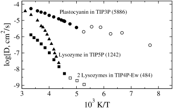
Figure 7: Diffusion coefficient of TIP3P water calculated from all $N_{w}=5886$ water molecules in the simulation box (circles). The triangles indicate the results of Ref. Kumar et al., 2006 for the simulation box containing $N_{w}=1242$ waters; the squares denote the results from Ref. Lagi et al., 2008 with $N_{w}=484$ per simulation box containing two protein molecules. Closed and open points indicate temperatures above and below the dynamical transition temperature, respectively.

The diffusion coefficient of water in the simulation box is plotted separately vs the inverse temperature in Fig. 7, where we also compare our results to previous simulations by Kumar et al Kumar et al. (2006) and by Lagi et al Lagi et al. (2008). The diffusion coefficient was calculated from the Einstein equation and the reported values are averaged over all waters in the simulation box. The different magnitudes of diffusivity compared to previous reports Kumar et al. (2006); Lagi et al. (2008) are related to the different force fields used, but, more importantly, to the different fractions of water molecules in the simulation sample. Given that all molecules in the smallest sample in Fig. 7 belong to the interface Lagi et al. (2008), it is not that surprising that these data show the slowest diffusion, in agreement with the common expectation of slower diffusion of waters in thin interfacial layers Sinha et al. (2008). Nevertheless, despite the use of a much larger number of waters ($N_{w}=5886$ vs $N_{w}=484$), we confirm here the existence of a crossover in the Arrhenius slope of water’s diffusion coefficient observed earlier in Ref. Lagi et al., 2008.

Two observations are relevant in respect to the diffusivity data shown in Fig. 7. First, the temperature law is Arrhenius both above and below the transition temperature with the slope decreasing at lower temperatures, in accord with previous observations Chen et al. (2006a); Lagi et al. (2008). Second, the transition temperature is shifted down to 200 K compared to 220 K found in simulations of partially hydrated proteins in Ref. Lagi et al., 2008. The first observation implies that we observe only a change in the character of a secondary, Arrhenius relaxation, as indeed often seen for electron transfer in proteins Parak et al. (1980), instead of a fragile-to-strong transition. This fact might be related to the often reported Ngai and Capaccioli (2007) disappearance of $\alpha$ relaxation in confined water most closely related to our simulation conditions. Since $D(T)$ follows closely the decrease in the number of hydration-shell waters (Fig. 6) a connection of the break in the slope to a secondary process produced by collective density fluctuations of the hydration shell seems a reasonable explanation. The second feature might imply that the existence and position of the transition temperature depends on the fraction of surface waters in the system. While all waters in the simulation setup in Ref. Lagi et al., 2008 belonged to the surface, only roughly 10% of waters in our simulations find themselves in the first solvation shell (Fig. 3 and Table 1). Likewise, we have obtained a fragile-to-strong crossover by considering only first-shell fluctuations in Fig. 5, but it is already washed out for the diffusivity averaged over several hydration layers.

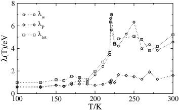
Figure 8: Reorganization energy obtained from the variance of the Coulomb energy gap: water component $\lambda_{w}$ [circles, Eq. (3)], the protein component $\lambda_{P}$ from the variance of $\Delta E^{C}_{P}$ (diamonds) and the total water/protein reorganization energy $\lambda_{\text{tot}}$ from the variance of the total Coulomb energy gap $\Delta E^{C}_{w}+\Delta E_{P}^{C}$ (squares).

Our data, while pointing mostly to the interfacial effects as the reason for the dramatic rise of $\lambda_{w}(T)$, do not entirely exclude crossing the Widom line, a bulk property of water, from the picture. While the global rise of the intensity of electrostatic fluctuations within protein is linked to the density fluctuations of the interface, the spike of $\lambda_{w}(T)$ at $T=220$ K and the corresponding slowing down of the Stokes shift relaxation might well be linked to the crossing of the Widom line. The increased cooperativity of water’s fluctuations at this temperature causes a behavior similar to the critical slowing down with a peak in a second energy cumulant, heat capacity for bulk measurements Kumar et al. (2006) and reorganization energy in our case.

The spike of $\lambda_{w}(T)$, barely seen on the 1 ns observation window, becomes more pronounced on the 10 ns time-scale, as is shown in Fig. 8 where the reorganization energies for water, protein, and the full reorganization energy from water/protein electrostatic fluctuations were collected from the entire 10 ns trajectories by calculating the variance of the total Coulomb energy gap $\Delta E_{w}^{C}+\Delta E_{P}^{C}$. This observation suggests that some collective motions of water, significantly cut off on the 1 ns time-scale, contribute to the peak and become more pronounced on a longer observation scale.

V Conclusions

In conclusion, we have found a dramatic increase in the breadth of water-induced electrostatic fluctuations inside the protein with increasing temperature. We link this increase to the creation of the hydrophobic interface at extended hydrophobic patches of the protein. What has escaped the attention of all studies of the dynamical transition in biopolymers is the onset of hydrophobic solvation occurring at the same temperature $T_{\text{tr}}$ as the dynamical transition. It might be true that the creation of the hydrophobic interface with its large extent of density fluctuations and intense electrostatic noise is closely linked to the dynamical transition, although we do not currently have any additional data supporting this view. However, if this view is correct, there should be a critical polypeptide dimension below which the macroscopic hydrophobic interface does not form Chandler (2005) and no dynamical transition exists. In fact, very recent measurements of terahertz dielectric response He and Markelz of hydrated polypeptides of different lengths have indicated the existence of an exactly such critical polymer length below which the dynamical transition disappears.

We found that the dynamics of electrostatic fluctuations are coupled to fast $\beta$ relaxation of the hydration shell. The redox activity of proteins can therefore be classified as hydration-shell-coupled, according to the classification suggested by Fenimore et al Fenimore et al. (2004). Although this coupling carries similarities with aqueous mixtures of simple glass-formers Ngai et al. (2008), proteins are not just large molecules. The formation of the hydrophobic interface is related to a particular lengthscale of hydrophobic patches ($\simeq 1$ nm Chandler (2005)) which does not exist for small hydrated molecules. Not surprisingly, large-amplitude electrostatic fluctuations observed here are not usually seen inside small molecules Matyushov (2007), although this feature might extend to other patchy hydrophobic surfaces, such as lipid membranes and dendrimeric structures.

It remains to be seen whether and how the gigantic reorganization energy found at high temperatures is related to the biological function of metalloproteins belonging to energetic electron-transfer chains. One can anticipate, from a general perspective, that a significant increase in the amplitude of electrostatic fluctuations can help in reducing barriers for chemical transformations by allowing better chances for favorable configurations from a broad fluctuation spectrum.