Analysis of a stochastic chemical system close to a SNIPER bifurcation of its mean-field model

Abstract

A framework for the analysis of stochastic models of chemical systems for which the deterministic mean-field description is undergoing a saddle-node infinite period (SNIPER) bifurcation is presented. Such a bifurcation occurs for example in the modelling of cell-cycle regulation. It is shown that the stochastic system possesses oscillatory solutions even for parameter values for which the mean-field model does not oscillate. The dependence of the mean period of these oscillations on the parameters of the model (kinetic rate constants) and the size of the system (number of molecules present) is studied. Our approach is based on the chemical Fokker-Planck equation. To get some insights into advantages and disadvantages of the method, a simple one-dimensional chemical switch is first analyzed, before the chemical SNIPER problem is studied in detail. First, results obtained by solving the Fokker-Planck equation numerically are presented. Then an asymptotic analysis of the Fokker-Planck equation is used to derive explicit formulae for the period of oscillation as a function of the rate constants and as a function of the system size.

1 Introduction

Bifurcation diagrams are often used for the analysis of deterministic models of chemical systems. In recent years, they have also been applied to models of biological (biochemical) systems. For example, the cell-cycle model of Tyson et al. [13] is a system of ordinary differential equations (ODEs) which describes the time evolution of concentrations of biochemical species involved in cell-cycle regulation. The dependence of the qualitative behaviour on the parameters of the model is studied using standard bifurcation analysis of ODEs [2, 3]. Biological systems are intrinsically noisy because of the low copy numbers of some of the biochemical species involved. In such a case, one has to use stochastic simulation algorithms (SSAs) to include the intrinsic noise in the modelling [6]. The SSA models use the same set of parameters as the ODE models. However, even if we choose the same values of the rate constants for both the SSA model and the ODE model, the behaviour of the system can differ qualitatively [1]. For example, the transition from the $G_{2}$ phase to mitosis in the model of Tyson et al. is governed by a SNIPER (saddle-node infinite period) bifurcation [13]. In the ODE setting, a SNIPER bifurcation occurs whenever a saddle and a stable node collapse into a single stationary point on a closed orbit (as a bifurcation parameter is varied). In particular, the limit cycle is born with infinite period at the bifurcation point. If we use the SSA model instead of ODEs, the bifurcation behaviour will be altered. As we will see in Section 2, intrinsic noise causes oscillations with finite average period at the deterministic bifurcation point. Moreover, the stochastic system oscillates even for the parameter values for which the deterministic model does not have a periodic solution. Clearly, there is a need to understand the changes in the bifurcation behaviour if a modeller decides to use SSAs instead of ODEs. In this paper, we focus on the SNIPER bifurcation. However, the approach presented can be applied to more general chemical systems.

In Section 2, we introduce a simple chemical system for which the ODE model undergoes a SNIPER bifurcation. We use this illustrative example to motivate the phenomena which we want to study. The study of stochastic chemical systems in the neighbourhood of determistic bifurcation points will be done using the chemical Fokker-Planck equation [7]. The analysis of the Fokker-Planck equation is much easier in one dimension. Thus, we start with an analysis of a simple one-dimensional chemical switch in Section 3. Using the one-dimensional setting, we can show some advantages and disadvantages of our approach without going into technicalities. In Section 4, we present a computer assisted analysis of the SSAs by exploiting the chemical Fokker-Planck equation, using the illustrative model from Section 2. In Section 5, we provide core analytical results. We study the dependence of the period of oscillation on the parameters of the model, namely kinetic rate constants and the size of the system (number of molecules present). We derive analytical formulae for the period of oscillation using the asymptotic expansion of the two-dimensional Fokker-Planck equation. Finally, in Section 6, we present our conclusions.

2 A chemical system undergoing a SNIPER bifurcation

We consider two chemical species $X$ and $Y$ in a well-mixed reactor of volume $V$ which are subject to the following set of seven chemical reactions

$$\mbox{ \raise 2.84526pt\hbox{ $\emptyset\;\displaystyle\mathop{\displaystyle\longrightarrow}^{k_{1d}}\;Y\;\displaystyle\mathop{\displaystyle\longrightarrow}^{k_{2d}}\;X\;\displaystyle\mathop{\displaystyle\longrightarrow}^{k_{3d}}\;\emptyset,$} }\qquad\qquad\qquad{\mbox{ \raise 2.42131pt\hbox{$2X$}}}\;\mathop{\stackrel{{\scriptstyle\displaystyle\longrightarrow}}{{\longleftarrow}}}^{k_{4d}}_{k_{5d}}\;{\mbox{\raise 2.42131pt\hbox{$3X,$}}}\qquad\qquad$$ (1)

$$X+Y\;\displaystyle\mathop{\displaystyle\longrightarrow}^{k_{6d}}\;X+2Y,\qquad\qquad\qquad\quad 2X+Y\;\displaystyle\mathop{\displaystyle\longrightarrow}^{k_{7d}}\;2X.\qquad$$ (2)

The first reaction is the production of the chemical $Y$ from a source with constant rate $k_{1d}$ per unit of volume, i.e. the units of $k_{1d}$ are $\mbox{sec}^{-1}\mbox{mm}^{-3}$, see (5) below. The second reaction is the conversion of $Y$ to $X$ with rate constant $k_{2d}$ and the third reaction is the degradation of $X$ with rate constant $k_{3d}$. The remaining reactions are of second-order or third-order. They were chosen so that the mean-field description corresponding to (1)–(2) undergoes a SNIPER bifurcation as shown below. Clearly, there exist many other chemical models with a SNIPER bifurcation, including the more realistic model of the cell-cycle regulation [13]. The advantage of the model (1)–(2) is that it involves only two chemical species $X$ and $Y$, making the visualization of our results clearer: two-dimensional phase planes are much easier to plot than the phase spaces of high-dimensional models. The generalization of our results to models involving more than two chemical species will be discussed in Section 6.

Let $X\equiv X(t)$ and $Y\equiv Y(t)$ be the number of molecules of the chemical species $X$ and $Y$, respectively. The concentration of $X$ (resp. $Y$) will be denoted by $\widetilde{x}=X/V$ (resp. $\widetilde{y}=Y/V$). If we have enough molecules of $X$ and $Y$ in the system, we often describe the time evolution of $\widetilde{x}$ and $\widetilde{y}$ by the mean-field ODE model. Using (1)–(2), this can be written as

$$\frac{\mbox{d}\widetilde{x}}{\mbox{d}t} = k_{2d}\,\widetilde{y}-k_{5d}\,\widetilde{x}^{\raise 1.42262pt\hbox{{\scriptsize 3}}}+k_{4d}\,\widetilde{x}^{\raise 1.42262pt\hbox{{\scriptsize 2}}}-k_{3d}\,\widetilde{x},$$ (3)

$$\frac{\mbox{d}\widetilde{y}}{\mbox{d}t} = -k_{7d}\,\widetilde{x}^{\raise 1.42262pt\hbox{{\scriptsize 2}}}\,\widetilde{y}+k_{6d}\,\widetilde{x}\,\widetilde{y}-k_{2d}\,\widetilde{y}+k_{1d}.$$ (4)

We choose the values of the rate constants as follows:

$$k_{1d}=12\;[\mbox{sec}^{-1}\,\mbox{mm}^{-3}],\quad k_{2d}=1\;[\mbox{sec}^{-1}],\quad k_{3d}=33\;[\mbox{sec}^{-1}],\quad k_{4d}=11\;[\mbox{sec}^{-1}\,\mbox{mm}^{3}],$$

$$k_{5d}=1\;[\mbox{sec}^{-1}\,\mbox{mm}^{6}],\quad k_{6d}=0.6\;[\mbox{sec}^{-1}\,\mbox{mm}^{3}],\quad k_{7d}=0.13\;[\mbox{sec}^{-1}\,\mbox{mm}^{6}],$$ (5)

where we have included the units of each rate constant to emphasize the dependence of each rate constant on the volume. From now on, we will treat all rate constants as numbers, dropping the corresponding units, to simplify our notation. The nullclines of the ODE system (3)–(4) are plotted in Figure 1(a). The $x$-nullcline (resp. $y$-nullcline) is given by $d\widetilde{x}/dt=0$ (resp. $d\widetilde{y}/dt=0$). The nullclines intersect at three steady states which are denoted as SN (stable node), Saddle and UN (unstable node). We also plot illustrative trajectories which start close to each steady state (thin black lines).

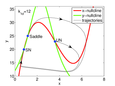
      (a) ​​​​ (b)

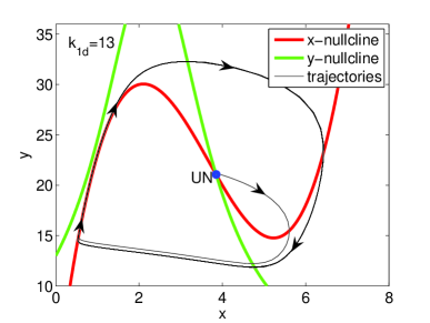
Fig. 1: Nullclines of the ODE system $(\ref{eq1})$–$(\ref{eq2})$ for $k_{1d}=12$ (left panel) and $k_{1d}=13$ (right panel). The other parameter values are given by $(\ref{sniperparam})$. The steady states are denoted by blue dots. Illustrative trajectories which start close to the steady states are plotted as thin black lines.

As the parameter values change, the stable node (SN) and the saddle can approach each other. If they coalesce into one point (with the dominant eigenvalue equal to 0), a limit cycle with infinite period appears. Shifting the nullclines further apart, we obtain a dynamical system with periodic solutions. This is demonstrated in Figure 1(b) where we plot the nullclines of (3)–(4) for $k_{1d}=13$, with the other parameter values given by $(\ref{sniperparam})$. An illustrative trajectory (thin black line) converges to the limit cycle. We see that there is a SNIPER (saddle-node infinite period) bifurcation as the parameter $k_{1d}$ is increased from 12 to 13.

The main goal of this paper is to understand and analyse changes in the behaviour of chemical systems when deterministic ODE models are replaced by SSAs, i.e. when the intrinsic noise is taken into account. The stochastic model of the chemical system (1)–(2) is given by the Gillespie SSA [6] which is equivalent to solving the corresponding chemical master equation – see Appendix A. We denote the reaction with the rate constant $k_{id}$, $i=1,2,\dots,7$, as the reaction $R_{i}$. Note that the reversible reaction in (1) is considered as two separate chemical reactions. To use the Gillespie SSA, we have to specify the propensity function $\alpha_{i}(x,y)$, $i=1,2,\dots,7$, of each chemical reaction in (1)–(2). The propensity function is defined so that $\alpha_{i}(x,y)\,\mbox{d}t$ is the probability that, given $X(t)=x$ and $Y(t)=y$, one $R_{i}$ reaction will occur in the next infinitesimal time interval $[t,t+\mbox{d}t)$. For example, $k_{1d}$ is the rate of production of $Y$ molecules per unit of volume. Thus, $k_{1}=k_{1d}V$ is the rate of production of $Y$ molecules per the whole reactor of volume $V$. Consequently, the probability that one $Y$ molecule is produced in the infinitesimally small time interval $[t,t+\mbox{d}t)$ is equal to $k_{1}\mbox{d}t$, i.e. the propensity function of the reaction $R_{1}$ is $\alpha_{1}(x,y)\equiv k_{1}=k_{1d}V.$ To specify other propensity functions, we first scale the rate constant $k_{id}$ with the appropriate power of the volume $V$, namely we define

$$k_{1}=k_{1d}V,\;\;k_{2}=k_{2d},\;\;k_{3}=k_{3d},\;\;k_{4}=\frac{k_{4d}}{V},\;\;k_{5}=\frac{k_{5d}}{V^{2}},\;\;k_{6}=\frac{k_{6d}}{V},\;\;k_{7}=\frac{k_{7d}}{V^{2}}.$$ (6)

Then the propensity function of the reaction $R_{i}$, $i=1,2,\dots,7$, is given as the product of the scaled rate constant and numbers of available reactant molecules, namely

$$\alpha_{1}(x,y)=k_{1},\;\;\alpha_{2}(x,y)=k_{2}y,\;\;\alpha_{3}(x,y)=k_{3}x,\;\;\alpha_{4}(x,y)=k_{4}x(x-1),$$

$$\alpha_{5}(x,y)=k_{5}x(x-1)(x-2),\;\;\alpha_{6}(x,y)=k_{6}xy,\;\;\alpha_{7}(x,y)=k_{7}x(x-1)y.$$ (7)

Note that the propensity functions of the reactions $R_{4}$ and $R_{7}$ are proportional to the number $x(x-1)/2$ of available pairs of $X$ molecules, and not to $x^{2}$; similarly, $\alpha_{5}$ is proportional to the number $x(x-1)(x-2)/6$ of available triplets of $X$ molecules and not to $x^{3}$. For a general discussion of the propensity functions see [6].

Using (7) and the Gillespie SSA, we can simulate the stochastic trajectories of (1)–(2). In Figure 2(a), we compare the time evolution of $X$ given by the stochastic (Gillespie SSA) and deterministic (the ODE system (3)–(4)) models. We use the same parameter values (5) and the same initial condition $[X,Y]=[40,480]$ for both, stochastic and deterministic, simulations. The reactor volume is $V=40$.

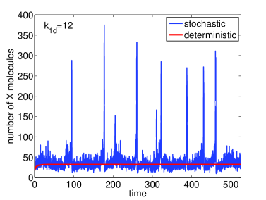
      (a)   (b)

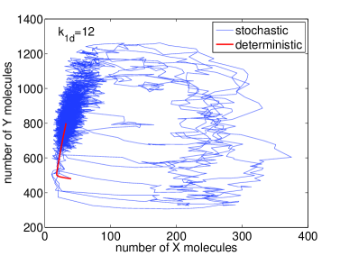
Fig. 2: (a) The time evolution of $X$ given by the stochastic (blue line) and deterministic (red line) models of the chemical system $(\ref{model1})$–$(\ref{model2})$. The rate constants are given by $(\ref{sniperparam})$ and $V=40.$ (b) The same trajectory plotted in the $X$-$Y$ plane.

In Figure 2(b), we plot both trajectories in the $x$-$y$ plane. We see that the solution of the deterministic equations converges to a steady state while the stochastic model has oscillatory solutions. In Figure 3, we present results obtained by the stochastic simulation of (1)–(2) for $k_{1d}=13$. The other parameters are the same as in Figure 2. We see that both the stochastic and deterministic models oscillate for $k_{1d}=13$.

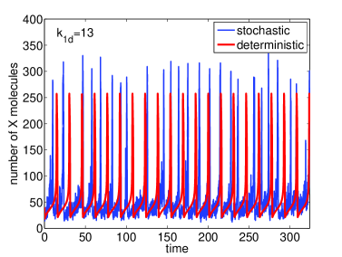
      (a)   (b)

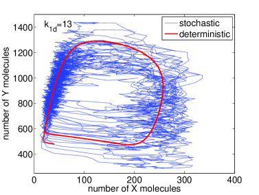
Fig. 3: (a) The time evolution of $X$ given by the stochastic (blue line) and deterministic (red line) models of the chemical system $(\ref{model1})$–$(\ref{model2})$ for $k_{1d}=13$. The other parameters are chosen as in Figure 2. (b) The same trajectory plotted in the $X$-$Y$ plane.

An important characteristic of oscillating systems is their period of oscillation. This is a well-defined number for the deterministic ODE model, but in the stochastic case the periods of individual oscillations vary. Thus, in the stochastic model we are interested in the mean period of oscillation (averaged over many periods). The mean period of oscillation is plotted in Figure 4(a) as a function of the rate constant $k_{1d}$ (blue circles). It was computed as an average over 10,000 periods for each of the presented values of $k_{1d}$. The starting/finishing point of every period was defined as the time when the simulation enters the half-plane $X>200$. More precisely, we start the computation of each period whenever the trajectory enters the area $X>200$. Then we wait until $X<60$ before we test the condition $X>200$ again. The extra condition $X<60$ guarantees that possible small random fluctuations around the point $X=200$ are not counted as two or more periods. The period of oscillation of the ODE model (3)–(4) is plotted in Figure 4(a) as the red line. It asymptotes to infinity as $(k_{1d}-K_{d})^{-1/2}$ for $k_{1d}\to K_{d}^{+}$ where $K_{d}\doteq 12.2$ is the bifurcation value of the parameter $k_{1d}$.

In the limit $V\to\infty$ (which is the so-called thermodynamic limit [7]), the stochastic description converges to the ODE model $(2.3)$-$(2.4)$, that is, the probability distributions become Dirac-like and their averages converge to the solution of the ODEs $(2.3)$-$(2.4)$ for $V\to\infty$. The dependence of the period of oscillation on the volume $V$ is shown in Figure 4(b) where we fix $k_{1d}$ equal to the bifurcation value $K_{d}\doteq 12.2$ of the ODE model and we vary the volume $V$. The other parameter values are given by $(\ref{sniperparam})$. Since $k_{1d}=K_{d}$, the period of oscillation of the ODE model is infinity. In Figure 4(b), we see that the period of oscillation of the stochastic model is an increasing function of $V$. It approaches the period of oscillation of the ODE model (infinity) as $V\to\infty$.

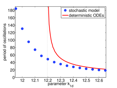
      (a) ​​​​ (b)

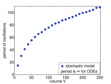
Fig. 4: (a) The mean period of oscillation of the chemical system $(\ref{model1})$–$(\ref{model2})$ as a function of the parameter $k_{1d}$. The other parameters are given by $(\ref{sniperparam})$ and $V=40.$ Each blue circle was obtained as an average over 10,000 periods of the stochastic model. The mean period of oscillation of the ODE model $(\ref{eq1})$–$(\ref{eq2})$ is plotted as the red line. (b) The period of oscillation as a function of the volume $V$. We use $k_{1d}=K_{d}\doteq 12.2$. Parameters $k_{2d},\dots,k_{7d}$ are given by $(\ref{sniperparam})$.

The estimates of the period of oscillation (blue circles in Figure 4) were obtained as averages over 10,000 periods of the Gillespie SSA. Such an approach is computationally intensive. The goal of this paper is to show that we can obtain the same information by solving and analyzing the chemical Fokker-Planck equation. In Section 4, we present results obtained by solving the Fokker-Planck equation using a suitable finite element method. In Section 5, we use the asymptotic analysis of the Fokker-Planck equation to derive explicit formulae for the period of oscillation, as a function of the rate constants and as a function of the volume $V$. The chemical Fokker-Planck equation which corresponds to the chemical system (1)–(2) is a two-dimensional partial differential equation. In particular, some parts of its analysis are more technical than the analysis of one-dimensional problems. To get some insights into our approach, we analyse a one-dimensional chemical switch in the following section. We will present only methods which are of potential use in the higher-dimensional settings. A generalization of the analysis to the chemical SNIPER problem is shown in Section 5.

3 One-dimensional chemical switch

We consider a chemical $X$ in a container of volume $V$ which is subject to the following set of chemical reactions (such a system was introduced by Schlögl [12])

$$\emptyset\;\mbox{ \raise-1.70717pt\hbox{$\displaystyle\mathop{\stackrel{{\scriptstyle\displaystyle\longrightarrow}}{{\longleftarrow}}}^{k_{1d}}_{k_{2d}}$}}\;\;X,\qquad\qquad\qquad 2X\;\mbox{ \raise-1.70717pt\hbox{$\displaystyle\mathop{\stackrel{{\scriptstyle\displaystyle\longrightarrow}}{{\longleftarrow}}}^{k_{3d}}_{k_{4d}}$}}\;\;3X.$$ (8)

Let $X(t)$ be the number of molecules of the chemical $X$. The classical deterministic description of the chemical system (8) is given by the following mean-field ODE for the concentration $\widetilde{x}=X/V$:

$$\frac{\mbox{d}\widetilde{x}}{\mbox{d}t}=k_{1d}-k_{2d}\,\widetilde{x}+k_{3d}\,\widetilde{x}^{\raise 1.42262pt\hbox{{\scriptsize 2}}}-k_{4d}\,\widetilde{x}^{\raise 1.42262pt\hbox{{\scriptsize 3}}}.$$ (9)

To obtain the stochastic description, we first scale the rate constants with the appropriate powers of the volume $V$, by defining

$$k_{1}=k_{1d}V,\qquad k_{2}=k_{2d},\qquad k_{3}=\frac{k_{3d}}{V},\qquad k_{4}=\frac{k_{4d}}{V^{2}}.$$ (10)

Then the propensity functions of the chemical reactions (8) are given by

$$\alpha_{1}(x)=k_{1},\;\,\alpha_{2}(x)=k_{2}x,\;\,\alpha_{3}(x)=k_{3}x(x-1),\;\,\alpha_{4}(x)=k_{4}x(x-1)(x-2),$$ (11)

i.e. the probability that, given $X(t)=x$, the $i$-th reaction occurs in the time interval $[t,t+\mbox{d}t)$ is equal to $\alpha_{i}(x)\;\mbox{d}t$. Given the propensity functions (11), we can simulate the time evolution of the system (8) by the Gillespie SSA [6]. We choose $V=1$ in what follows, i.e. $k_{i}=k_{id}$, $i=1,2,3,4.$ In Figure 5(a), we plot illustrative results obtained by the Gillespie SSA for the following set of rate constants

$$k_{1}=2250,\qquad k_{2}=37.5,\qquad k_{3}=0.18,\qquad k_{4}=2.5\times 10^{-4}.$$ (12)

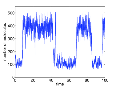
      (a) ​​​​ (b)

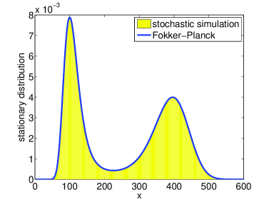
Fig. 5: (a) Time evolution of $X$ obtained by the Gillespie SSA for the chemical system $(\ref{schlogl})$. The values of the rate constants are given by $(\ref{paramschlogl})$. (b) Stationary distribution of $(\ref{schlogl})$ obtained by the Gillespie SSA (yellow histogram) for the parameters $(\ref{paramschlogl})$. The blue curve is the stationary solution $(\ref{Psvd})$ of the chemical Fokker-Planck equation.

We see that the system (8) has two favourable states for the parameter values (12). We also plot stationary distributions (yellow histograms) obtained by long time simulation of the Gillespie SSA in Figure 5(b). The chemical master equation corresponding to (8) can be written as follows

$$\frac{\partial}{\partial t}p(x,t)=\sum_{i=1}^{4}\Big{[}\alpha_{i}(x+(-1)^{i})\,p(x+(-1)^{i},t)-\alpha_{i}(x)p(x,t)\Big{]}$$ (13)

where $p(x,t)$ is the probability that $X(t)=x$, i.e. the probability that there are $x$ molecules of the chemical species $X$ at time $t$ in the system. The stationary solution of this infinite set of ODEs can be found in a closed form [10], i.e. one can find an exact formula for the stationary distribution plotted in Figure 5(b). However, our goal is not to solve the well-known Schlögl system using its master equation. We want to motivate the approach which is used later for the chemical SNIPER problem, which is based on the approximate description of chemical systems given by the chemical Fokker-Planck equation [7], see Appendix A. To write this equation, we have to consider $p(x,t)$ as a function of the real variable $x$, i.e. we smoothly extend the function $p(x,t)$ to non-integer values of $x$. Using Appendix A, the chemical Fokker-Planck equation for the chemical system (8) is

$$\frac{\partial p}{\partial t}(x,t)=\frac{\partial^{2}}{\partial x^{2}}\Big{(}d(x)p(x,t)\Big{)}-\frac{\partial}{\partial x}\Big{(}v(x)p(x,t)\Big{)}$$ (14)

where the drift coefficient $v(x)$ and the diffusion coeficient $d(x)$ are given by

$$v(x)=\sum_{i=1}^{4}(-1)^{i+1}\alpha_{i}(x)=k_{1}-k_{2}\,x+k_{3}\,x(x-1)-k_{4}\,x(x-1)(x-2),$$ (15)

$$d(x)=\frac{1}{2}\sum_{i=1}^{4}\alpha_{i}(x)=\frac{k_{1}+k_{2}\,x+k_{3}\,x(x-1)+k_{4}\,x(x-1)(x-2)}{2}.$$ (16)

The stationary distribution $P_{s}(x)=\lim_{t\to\infty}p(x,t)$ is a solution of the stationary equation corresponding to (14), namely

$$\frac{\mbox{d}^{2}}{\mbox{d}x^{2}}\Big{(}d(x)P_{s}(x)\Big{)}-\frac{\mbox{d}}{\mbox{d}x}\Big{(}v(x)P_{s}(x)\Big{)}=0.$$ (17)

Integrating over $x$ and using the boundary conditions $P_{s}(x)\to 0$ as $x\to\pm\infty$, we obtain

$$P_{s}(x)=\frac{c}{d(x)}\exp\left[\int_{0}^{x}\frac{v(z)}{d(z)}\,\mbox{d}z\right]$$ (18)

where $c$ is the constant given by the normalization $\int_{\mathbb{R}}P_{s}(x)\mbox{d}x=1.$ The function $P_{s}$ is plotted in Figure 5(b) for comparison as the blue line. We see that the chemical Fokker-Planck equation gives a very good description of the chemical system (8).

The Fokker-Planck equation (14) is equivalent to the Langevin equation (Itô stochastic differential equation)

$$\mbox{\mbox{d}X}=v(X)\,\mbox{d}t+\sqrt{2d(X)}\,\mbox{d}W$$

where $dW$ represents white noise. In particular, the deterministic part of the dynamics is given by the ODE $\mbox{d}X/dt=v(X).$ Substituting (15) for $v(X)$, using (10) and dividing by $V$, we obtain the following ODE for the concentration $\widetilde{x}=X/V$:

$$\frac{\mbox{d}\widetilde{x}}{\mbox{d}t}=k_{1d}-k_{2d}\,\widetilde{x}+k_{3d}\,\widetilde{x}\left(\widetilde{x}-\frac{1}{V}\right)-k_{4d}\,\widetilde{x}\left(\widetilde{x}-\frac{1}{V}\right)\left(\widetilde{x}-\frac{2}{V}\right).$$ (19)

This equation slightly differs from the classical mean-field deterministic description (9), but the equations (9) and (19) are equivalent in the limit of large $X$ in which $\widetilde{x}\gg 1/V$. This can also be thought of as the limit of large $V$ after a suitable non-dimensionalization. Let us note that the chemical Fokker-Planck equation is actually derived from the Kramers-Moyal expansion in the limit of large $V$ by keeping only the first and the second derivatives in the expansion [7].

3.1 Mean switching time

Let $x_{f1}$ and $x_{f2}$ be favourable states of the chemical system (8) which we define as the arguments of the maxima of $P_{s}$ (given by (18)). Let $x_{u}$ be the local minimum of $P_{s}$ which lies between the two favourable states, so that $x_{f1}<x_{u}<x_{f2}$. We can find the local extrema $x_{f1},$ $x_{u}$ and $x_{f2}$ of $P_{s}$ as the solutions of $P_{s}^{\prime}(x)=0$, which, using (18), is equivalent to the cubic equation

$$v(x)-d^{\prime}(x)=0.$$ (20)

Another way to define the favourable states of the system is by considering the stationary points of the ODE (19), i.e. the points where the drift coefficient is zero:

$$v(x)=k_{1}-k_{2}\,x+k_{3}\,x(x-1)-k_{4}\,x(x-1)(x-2)=0.$$ (21)

This cubic equation has three roots which we denote $y_{f1}$, $y_{u}$ and $y_{f2}$, where $y_{f1}<y_{u}<y_{f2}.$ Let us note that $x_{f1}\neq y_{f1}$, $x_{u}\neq y_{u}$ and $x_{f2}\neq y_{f2}$ because the equation (20) differs from the equation (21) by the additional term $d^{\prime}(x)$. In Figure 6(a), we plot $y_{f1},$ $y_{u},$ $y_{f2}$ as functions of $k_{1}$. The other parameter values are chosen as in (12).

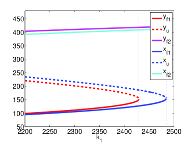
      (a) ​​​​ (b)

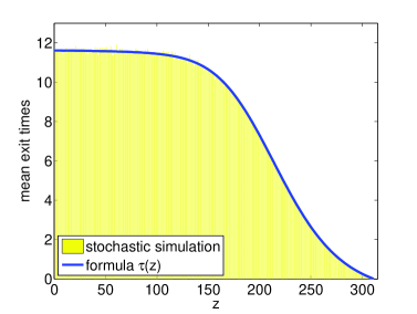
Fig. 6: (a) The local extrema of the potential (i.e. the solutions $x_{f1}<x_{u}<x_{f2}$ of the equation $(\ref{xfueq})$) and the solutions $y_{f1}<y_{u}<y_{f2}$ of the equation $v(y)=0$ as functions of the parameter $k_{1}$. The critical values $K$ and $K_{x}$ are plotted as the blue dotted lines. (b) Mean exit times $\tau(z)$ to leave the interval $(-\infty,(x_{u}+x_{f2})/2)$, given that initially $X(0)=z$. We compare the results obtained by the Gillespie SSA (yellow histogram, averages over $10^{4}$ exits for each $z$) with the results obtained by the formula $(\ref{tauzformula})$ (blue curve). Parameter values are given by $(\ref{paramschlogl})$.

We also plot $x_{f1},$ $x_{u},$ $x_{f2}$. We see that there are two critical values of the parameter $k_{1}$, namely $K\doteq 2429.35$ and $K_{x}\doteq 2484.39$. If $k_{1}=K$, then $y_{f1}=y_{u}$, while if $k_{1}=K_{x}$, then $x_{f1}=x_{u}$, i.e. the number of local maxima of $P_{s}$ changes at $k_{1}=K_{x}$. From our point of view, the more interesting critical value is $K$, corresponding to the bifurcation value of the deterministic description (19), but it is important to note that this value differs from the value $K_{x}$. To find the value of $K$, we solve the quadratic equation $v^{\prime}(x)=0$. The relevant root is given by:

$$y_{k}=1+\frac{k_{3}}{3k_{4}}-\frac{1}{6k_{4}}\sqrt{(6k_{4}+2k_{3})^{2}-12k_{4}(2k_{4}+k_{3}+k_{2})}.$$ (22)

The value of $K$ is determined by the equation $y_{f1}=y_{u}=y_{k}$, giving

$$K=k_{4}\,y_{k}(y_{k}-1)(y_{k}-2)-k_{3}\,y_{k}(y_{k}-1)+k_{2}\,y_{k}.$$

For the parameter values (12), we obtain $y_{k}\doteq 152.45$ and $K\doteq 2429.35.$

Let $\tau(y)$ be the average time to leave the interval $(-\infty,b)$ given that we start at $X(0)=y$. Using the backward Kolmogorov equation (adjoint equation to the Fokker-Planck equation (14)), one can derive a differential equation for $\tau(y)$ (see [5] and also Appendix B), namely

$$-1=v(y)\frac{\mbox{d}\tau}{\mbox{d}y}(y)+d(y)\frac{\mbox{d}^{2}\tau}{\mbox{d}y^{2}}(y)\qquad\mbox{for}\;y\in(-\infty,b),$$ (23)

with boundary conditions

$$\frac{\mbox{d}\tau}{\mbox{d}y}(-\infty)=0,\qquad\tau(b)=0.$$ (24)

Solving (23), we obtain

$$\frac{\mbox{d}\tau}{\mbox{d}y}(y) = -\exp\left[-\int_{0}^{y}\frac{v(z)}{d(z)}\,\mbox{d}z\right]\int_{-\infty}^{y}\frac{1}{d(x)}\exp\left[\int_{0}^{x}\frac{v(z)}{d(z)}\,\mbox{d}z\right]\mbox{d}x$$

$$= -\frac{1}{d(y)P_{s}(y)}\int_{-\infty}^{y}P_{s}(x)\mbox{d}x,$$

where $P_{s}$ is the stationary distribution (18). Integrating over $y$ in the interval $(z,b)$ and using (24), we obtain

$$\tau(z)=-\int_{z}^{b}\frac{\mbox{d}\tau}{\mbox{d}y}(y)\mbox{d}y=\int_{z}^{b}\frac{1}{d(y)P_{s}(y)}\int_{-\infty}^{y}P_{s}(x)\mbox{d}x\mbox{d}y.$$ (25)

The important characteristic of the system is the mean time $T(k_{1})$ for the system to switch from the favourable state $x_{f1}$ to the favourable state $x_{f2}.$ To determine this we set

$$b=\left\{\begin{matrix}(x_{u}+x_{f2})/2,&\qquad\mbox{for}\;k_{1}<K_{x},\\ 284,&\qquad\mbox{for}\;k_{1}\geq K_{x},\end{matrix}\right.$$ (26)

and we define $T(k_{1})$ precisely as the mean time to leave the interval $(-\infty,b)$ given that $X(0)=0$. This definition provides a natural extension of the mean switching time for values $k_{1}>K_{x}$. Note that the number $284$ in (26) is the value of $(x_{u}+x_{f2})/2$ at the critical point $k_{1}=K_{x}$. Using (25), we can compute $T(k_{1})$ as the integral

$$T(k_{1})=\int_{0}^{b}\exp\left[-\int_{0}^{y}\frac{v(z)}{d(z)}\,\mbox{d}z\right]\int_{-\infty}^{y}\frac{1}{d(x)}\exp\left[\int_{0}^{x}\frac{v(z)}{d(z)}\,\mbox{d}z\right]\mbox{d}x\mbox{d}y$$ (27)

where $b$ is given by (26). Let us note that we could also put the right boundary $b$ at the points $x_{u}$ or $y_{u}$. If the number of molecules reaches the value $x_{u}$ (resp. $y_{u}$), then there is, roughly speaking, 50% chance to return back to the favourable state $x_{f1}$ and 50% chance to continue to the second favourable state $x_{f2}$. Thus the mean switching time between the states could be estimated by multiplying the time to reach the point $x_{u}$ (resp. $y_{u}$) by the factor of 2. The problem with this definition is that $x_{u}\neq y_{u}$. The difference between the results obtained by choosing the escape boundary at $x_{u}$ or $y_{u}$ is not negligible because the drift is small between $x_{u}$ and $y_{u}$. On the other hand, the drift is large at $(x_{u}+x_{f2})/2$. Replacing $(x_{u}+x_{f2})/2$ by any number close to it, e.g. by $(y_{u}+y_{f2})/2$, leads to negligible errors. In that sense, the boundary $b$ given by (26) yields a more robust definition of the mean switching time. The other reason for presenting analysis for the definition (27) is that it is naturally transferable to the chemical SNIPER problem which is the main interest of this paper.

In Figure 6(b), we compare the results obtained by the Gillespie SSA and by formula (25) for the parameter values (12) and the right boundary at $b=(x_{u}+x_{f2})/2=310.8$. We have $x_{f1}=99.9$, $x_{u}=225.6$ and $x_{f2}=396.0$ for the parameter values (12). In Figure 6(b), we plot mean exit times computed as averages over $10^{4}$ exits from the domain $[0,b]$, starting at $X(0)=z$ for every integer value of $z<b.$ The results are in excellent agreement with the results computed by the formula (25).

In Figure 6(b), we also see that there is no significant difference between the exit times if we start at $X(0)=x_{f1}$ or $X(0)=0$ for $k_{1}\ll K_{x}$. This justifies the choice $X(0)=0$ in the definition of the mean switching time $T(k_{1})$. If $k_{1}\approx K_{x}$, than $x_{f1}$ is close to $x_{u}$ and the results obtained by the starting point at $X(0)=0$ and at $X(0)=x_{f1}$ will differ. In the definition (27), we use $X(0)=0$ for any value of $k_{1}$ because (i) the results for $X(0)=0$ will provide some insights into the estimation of the period of oscillation of the SNIPER problem studied later; (ii) the results are robust to small changes in the initial condition $X(0)=0$; (iii) the starting point $X(0)=0$ is defined for any value of $k_{1}$ (note that $x_{f1}$ is not defined for $k_{1}>K_{x}$).

In the remainder of this section, we provide approximations of $T(k_{1})$ defined by the formula (27). We fix the parameters $k_{2}$, $k_{3}$ and $k_{4}$ as in (12) and we vary the parameter $k_{1}$. In Section 3.2, we provide the estimation of $T(k_{1})$ for $k_{1}\ll K$ (outer solution). In Section 3.3, we provide the estimation of $T(k_{1})$ for $k_{1}\approx K$ (inner solution). Finally, in Section 3.4, we match the inner and outer solutions to obtain the uniform approximation for any $k_{1}$.

We note here that one could approximate $T(k_{1})$ by approximating the integral (27). Using the method of steepest descent, we would obtain the generalization of the well-known Kramers formula

$$T(k_{1})\approx T_{k}(k_{1})\equiv\frac{2\pi\exp[\Phi(x_{u})-\Phi(x_{f1})]}{d(x_{u})\sqrt{\Phi^{\prime\prime}(x_{f1})|\Phi^{\prime\prime}(x_{u})|}}$$ (28)

where $\Phi(x)$ is defined by $\Phi(x)=-\int_{0}^{x}v(y)/d(y)\mbox{d}y+\log(d(x)).$ This approximation is valid for $k_{1}\ll K$ [11]. Haataja et al. [9] suggest another generalization of the Kramers formula replacing $d(x_{u})$ in the denominator of (28) by $\{d(x_{u})+d(x_{f1})\}/2$, but this approximation is worse than (28). Unfortunately, such an integral representation is not available for higher-dimensional Fokker-Planck equations, including the SNIPER problem studied later. Since our main goal is to present methods which are applicable in higher-dimensions also, in Sections 3.2, 3.3 and 3.4 we focus on approximating the mean switching time $T(k_{1})$ by analysing the $\tau$-equation (23). The chemical Fokker-Planck equation and the corresponding $\tau$-equation are available in any dimension – see Appendix A and Appendix B.

3.2 Approximation of the mean switching time $T(k_{1})$ for $k_{1}\ll K$

Formula (16) and the parameter values (12) imply that $d(x)$ is of the order $10^{4}$ while $x$ is of the order $10^{2}$. Considering small $\varepsilon\sim 10^{-2}$, we use the following scaling

$$v=\frac{\overline{v}}{\varepsilon^{2}},\qquad d=\frac{\overline{d}}{\varepsilon^{2}},\qquad y=\frac{\overline{y}}{\varepsilon},\qquad\tau=\varepsilon\,\overline{\tau}.$$ (29)

Then we can rewrite the equation (23) to

$$\overline{v}(\overline{y})\frac{\mbox{d}\overline{\tau}}{\mbox{d}\overline{y}}(\overline{y})+\varepsilon\overline{d}(\overline{y})\frac{\mbox{d}^{2}\overline{\tau}}{\mbox{d}\overline{y}^{2}}(\overline{y})=-1.$$ (30)

Later we will see that in fact $\overline{\tau}$ is exponentially large in $\varepsilon$, so that the left-hand side of this equation dominates the right-hand side. Then $\overline{\tau}$ will be approximately constant except when $\overline{v}\approx 0$, that is, the main variation in $\overline{\tau}$ occurs near $\overline{y}=\overline{y}_{u}$. For $\overline{y}$ close to $\overline{y}_{u}$, we use the transformation of variables $\overline{y}=\overline{y}_{u}+\sqrt{\varepsilon}\,\eta$ and approximate

$$\overline{v}(\overline{y})\approx\sqrt{\varepsilon}\,\eta\frac{\mbox{d}\overline{v}}{\mbox{d}\overline{y}}(\overline{y}_{u}),\qquad\overline{d}(\overline{y})\approx\overline{d}(\overline{y}_{u}),\qquad\overline{\tau}\gg 1,$$ (31)

to give

$$\eta\frac{\mbox{d}\overline{v}}{\mbox{d}\overline{y}}(\overline{y}_{u})\frac{\mbox{d}\overline{\tau}}{\mbox{d}\eta}(\eta)+\overline{d}(\overline{y}_{u})\frac{\mbox{d}^{2}\overline{\tau}}{\mbox{d}\eta^{2}}(\eta)=0.$$ (32)

Integrating over $\eta$, we get

$$\exp\left[\frac{1}{2\overline{d}(\overline{y}_{u})}\frac{\mbox{d}\overline{v}}{\mbox{d}\overline{y}}(\overline{y}_{u})\eta^{2}\right]\frac{\mbox{d}\overline{\tau}}{\mbox{d}\eta}=\frac{c_{1}}{\overline{d}(\overline{y}_{u})}$$ (33)

where $c_{1}$ is a real constant. To determine $c_{1}$ we cannot use the local expansion near $\overline{y}_{u}$ alone; $c_{1}$ is determined by the number $-1$ on the right-hand side of (30), which is the only place the scale of $\overline{\tau}$ is set. To determine $c_{1}$ we use the projection method of Ward [14]. The stationary Fokker-Planck equation (17) can be rewritten

$$-\frac{\mbox{d}}{\mbox{d}\overline{y}}\left[\overline{v}(\overline{y})P_{s}(\overline{y})\right]+\varepsilon\frac{\mbox{d}^{2}}{\mbox{d}\overline{y}^{2}}\left[\overline{d}(\overline{y})P_{s}(\overline{y})\right]=0,$$ (34)

which is the adjoint equation to the homogeneous version of (30). Multiplying the equation (30) by $P_{s}$, the equation (34) by $\overline{\tau}$, integrating over $\overline{y}$ in the interval $[-\infty,\overline{y}_{u}]$ and subtracting the resulting equations, we obtain

$$\int_{-\infty}^{\overline{y_{u}}}\frac{\mbox{d}}{\mbox{d}\overline{y}}\left[P_{s}(\overline{y})\overline{v}(\overline{y})\overline{\tau}(\overline{y})\right]\mbox{d}\overline{y}$$

$$+\,\varepsilon \int_{-\infty}^{\overline{y}_{u}}\left(\frac{\mbox{d}}{\mbox{d}\overline{y}}\left[P_{s}(\overline{y})\overline{d}(\overline{y})\frac{\mbox{d}\overline{\tau}}{\mbox{d}\overline{y}}(\overline{y})\right]-\frac{\mbox{d}}{\mbox{d}\overline{y}}\left[\overline{\tau}(\overline{y})\frac{\mbox{d}}{\mbox{d}\overline{y}}\left[\overline{d}(\overline{y})P_{s}(\overline{y})\right]\right]\right)\mbox{d}\overline{y}=-\int_{-\infty}^{\overline{y}_{u}}P_{s}(\overline{y})\mbox{d}\overline{y}.$$

Evaluating the integrals on the left hand side with the help of (34) and the boundary condition (24), we find

$$\frac{\mbox{d}\overline{\tau}}{\mbox{d}\overline{y}}(\overline{y}_{u})=-\frac{1}{\varepsilon P_{s}(\overline{y}_{u})\overline{d}(\overline{y}_{u})}\int_{-\infty}^{\overline{y}_{u}}P_{s}(\overline{y})\mbox{d}\overline{y}.$$ (35)

Since $P_{s}$ is exponentially localized near $\overline{y}_{f1}$ and $\overline{y}_{f2}$, $P_{s}(\overline{y}_{u})$ is exponentially small in $\varepsilon.$ Using (33) in (35), we find

$$c_{1}=\overline{d}(\overline{y}_{u})\frac{\mbox{d}\overline{\tau}}{\mbox{d}\eta}(0)=\sqrt{\varepsilon}\;\overline{d}(\overline{y}_{u})\frac{\mbox{d}\overline{\tau}}{\mbox{d}\overline{y}}(\overline{y}_{u})=-\frac{1}{\sqrt{\varepsilon}\,P_{s}(\overline{y}_{u})}\int_{-\infty}^{\overline{y}_{u}}P_{s}(\overline{y})\mbox{d}\overline{y},$$

so that

$$\frac{\mbox{d}\overline{\tau}}{\mbox{d}\eta}\approx-\frac{1}{\sqrt{\varepsilon}\,P_{s}(\overline{y}_{u})\overline{d}(\overline{y}_{u})}\,\exp\left[-\frac{1}{2\overline{d}(\overline{y}_{u})}\frac{\mbox{d}\overline{v}}{\mbox{d}\overline{y}}(\overline{y}_{u})\eta^{2}\right]\int_{-\infty}^{\overline{y}_{u}}P_{s}(\overline{y})\mbox{d}\overline{y}.$$

Integrating over $\eta$ in $[-\infty,\infty]$, we obtain

$$\lim_{\eta\to-\infty}\overline{\tau}(\eta)=\frac{\sqrt{2\pi}}{\sqrt{\varepsilon\overline{d}(\overline{y}_{u})}\,P_{s}(\overline{y}_{u})}\left(\frac{\mbox{d}\overline{v}}{\mbox{d}\overline{y}}(\overline{y}_{u})\right)^{\!\!\!-1/2}\int_{-\infty}^{\overline{y}_{u}}P_{s}(\overline{y})\mbox{d}\overline{y},$$ (36)

where we used that $\overline{\tau}(\eta)\to 0$ as $\eta\to\infty$, i.e. the switching time is going to zero if the starting point approaches the boundary $b$, see Figure 6(b). The limit $\eta\to-\infty$ on the left hand side of (36) is an approximation of the mean switching time $T(k_{1})$. It is the plateau value of $\tau(z)$ in Figure 6(b). Transforming (36) to the original variables, we obtain the following approximation for the mean switching time

$$T(k_{1})\approx T_{\mbox{\rm\scriptsize a}}(k_{1})\equiv\frac{\sqrt{2\pi}}{\sqrt{d(y_{u})}\,P_{s}(y_{u})}\left(\frac{\mbox{d}v}{\mbox{d}y}(y_{u})\right)^{\!\!\!-1/2}\int_{-\infty}^{y_{u}}P_{s}(y)\mbox{d}y.$$ (37)

Let us define the potential $\Psi$ by

$$\Psi(x)=-\int_{0}^{x}\frac{v(z)}{d(z)}\,\mbox{d}z.$$

Then (37) can be rewritten as

$$T_{\mbox{\rm\scriptsize a}}(k_{1})=\sqrt{2\pi d(y_{u})}\,\exp[\Psi(y_{u})]\left(\frac{\mbox{d}v}{\mbox{d}y}(y_{u})\right)^{\!\!\!-1/2}\int_{-\infty}^{y_{u}}\frac{\exp[-\Psi(y)]}{d(y)}\mbox{d}y.$$

The local extrema of the potential $\Psi$ are equal to $y_{f1}$, $y_{u}$ and $y_{f2}$. Using the Taylor expansion $\Psi(y)\approx\Psi(y_{f1})+(y-y_{f1})^{2}\Psi^{\prime\prime}(y_{f1})/2$ in the integral on the right hand side, we approximate

$$T(k_{1})\,\approx\,T_{\mbox{\rm\scriptsize a}}(k_{1})\,\approx\,\exp[\Psi(y_{u})-\Psi(y_{f1})]\left(\frac{\mbox{d}v}{\mbox{d}y}(y_{u})\right)^{\!\!\!-1/2}\frac{2\pi\sqrt{d(y_{u})}}{d(y_{f1})\sqrt{\Psi^{\prime\prime}(y_{f1})}}.$$

Using the definition of $\Psi$, we obtain the following approximation of the mean switching time

$$T(k_{1})\approx T_{o}(k_{1})\equiv 2\pi\sqrt{d(y_{u})}\,\exp\!\left[-\int_{y_{f1}}^{y_{u}}\frac{v(z)}{d(z)}\,\mbox{d}z\right]\left(\frac{\mbox{d}v}{\mbox{d}y}(y_{u})\left|\frac{\mbox{d}v}{\mbox{d}y}(y_{f1})\right|d(y_{f1})\right)^{\!\!\!-1/2}.$$ (38)

We will call $T_{o}(k_{1})$ the outer solution. In Figure 7(a), we compare the approximations

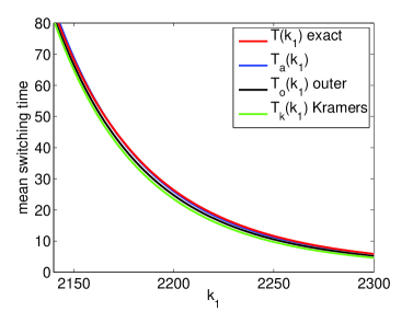
   (a) ​​​​ (b)

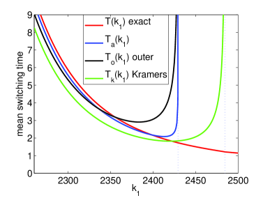
Fig. 7: Approximations $(\ref{tauKramers})$, $(\ref{tauappj})$ and $(\ref{tauouterapp})$ of the mean switching time $T(k_{1})$. The red line is the exact value given by $(\ref{taudef2})$. (a) Region $k_{1}\ll K$ for which the derivation was made. (b) Behaviour of approximations close to the critical points $k_{1}=K$ and $k_{1}=K_{x}$. The critical values $K$ and $K_{x}$ are plotted as the dotted lines, $K<K_{x}$.

(37) and (38) with the exact value given by $(\ref{taudef2})$. We see that $T_{\mbox{\rm\scriptsize a}}$ and $T_{o}$ provide good approximation of the mean switching time. In Figure 7(b), we present the behaviour of approximations close to the critical point $k_{1}=K$. They both blow up at the point $k_{1}=K$. We also plot the results obtained by the Kramers approximation $T_{k}(k_{1})$ given by (28). We again confirm that it provides a good approximation for $k_{1}\ll K$, see Figure 7(a), but it blows up at the point $k_{1}=K_{x}$, see Figure 7(b). In the next section, we present the inner approximation which is valid close to the critical point $k_{1}=K.$

3.3 Approximation of the mean switching time $T(k_{1})$ for $k_{1}\approx K$

If $k_{1}=K$, then $\overline{y}_{u}=\overline{y}_{f1}=\overline{y}_{k}$ where $y_{k}$ is given by (22). Consider the drift coefficient given as a function of $\overline{y}$ and the parameter $k_{1}$, namely

$$\overline{v}(\overline{y},k_{1})=k_{1}-k_{2}\,\overline{y}+k_{3}\,\overline{y}(\overline{y}-1)-k_{4}\,\overline{y}(\overline{y}-1)(\overline{y}-2).$$ (39)

If $\overline{y}$ is close to $\overline{y}_{k}$ and $k_{1}$ is close to $K$, we can use the Taylor expansion to approximate

$$\overline{v}(\overline{y},k_{1})\approx\frac{1}{2}\frac{\partial^{2}\overline{v}}{\partial\overline{y}^{2}}(\overline{y}_{k},K)\left(\overline{y}-\overline{y}_{k}\right)^{2}+(k_{1}-K),$$ (40)

where we used

$$\frac{\partial\overline{v}}{\partial k_{1}}(\overline{y}_{k},K)=1\;\;\;\mbox{and}\;\;\;\overline{v}(\overline{y}_{k},K)=\frac{\partial\overline{v}}{\partial\overline{y}}(\overline{y}_{k},K)=\frac{\partial^{2}\overline{v}}{\partial\overline{y}\partial k_{1}}(\overline{y}_{k},K)=\frac{\partial^{2}\overline{v}}{\partial k_{1}^{2}}(\overline{y}_{k},K)=0.$$

We use the transformation of variables $\overline{y}=\overline{y}_{k}+\varepsilon^{1/3}\,\eta$ and $k_{1}=K+\varepsilon^{2/3}\,\kappa$. Then (40) implies

$$\overline{v}(\overline{y},k_{1})\approx\varepsilon^{2/3}\left(\frac{1}{2}\frac{\partial^{2}\overline{v}}{\partial\overline{y}^{2}}(\overline{y}_{k},K)\eta^{2}+\kappa\right).$$ (41)

Now in (29) we need to replace $\tau=\varepsilon\,\overline{\tau}$ by $\tau=\varepsilon^{2/3}\,\overline{\tau}$. Then (30) reads as follows

$$\varepsilon^{-1/3}\overline{v}(\overline{y})\frac{\mbox{d}\overline{\tau}}{\mbox{d}\overline{y}}(\overline{y})+\varepsilon^{2/3}\overline{d}(\overline{y})\frac{\mbox{d}^{2}\overline{\tau}}{\mbox{d}\overline{y}^{2}}(\overline{y})=-1.$$ (42)

Using (41) and approximating $\overline{d}(\overline{y})\approx\overline{d}(\overline{y}_{k})$, we get

$$\left(\frac{1}{2}\frac{\partial^{2}\overline{v}}{\partial\overline{y}^{2}}(\overline{y}_{k},K)\eta^{2}+\kappa\right)\frac{\mbox{d}\overline{\tau}}{\mbox{d}\eta}(\eta)+\overline{d}(\overline{y}_{k})\frac{\mbox{d}^{2}\overline{\tau}}{\mbox{d}\eta^{2}}(\eta)=-1.$$ (43)

This time, since we are close to the bifurcation point, the right-hand side is not negligible. Equation (43) can be rewritten as

$$\frac{\mbox{d}}{\mbox{d}\eta}\left(\overline{d}(\overline{y}_{k})\exp\left[\frac{1}{\overline{d}(\overline{y}_{k})}\left(\frac{1}{2}\frac{\partial^{2}\overline{v}}{\partial\overline{y}^{2}}(\overline{y}_{k},K)\frac{\eta^{3}}{3}+\kappa\eta\right)\right]\frac{\mbox{d}\overline{\tau}}{\mbox{d}\eta}\right)$$

$$=-\exp\left[\frac{1}{\overline{d}(\overline{y}_{k})}\left(\frac{1}{2}\frac{\partial^{2}\overline{v}}{\partial\overline{y}^{2}}(\overline{y}_{k},K)\frac{\eta^{3}}{3}+\kappa\eta\right)\right].$$

Integrating over $\eta$, we get

$$\frac{\mbox{d}\overline{\tau}}{\mbox{d}\eta} = -\frac{1}{\overline{d}(\overline{y}_{k})}\exp\left[-\frac{1}{\overline{d}(\overline{y}_{k})}\left(\frac{1}{2}\frac{\partial^{2}\overline{v}}{\partial\overline{y}^{2}}(\overline{y}_{k},K)\frac{\eta^{3}}{3}+\kappa\eta\right)\right]$$ (44)

$$\times \int_{-\infty}^{\eta}\exp\left[\frac{1}{\overline{d}(\overline{y}_{k})}\left(\frac{1}{2}\frac{\partial^{2}\overline{v}}{\partial\overline{y}^{2}}(\overline{y}_{k},K)\frac{\xi^{3}}{3}+\kappa\xi\right)\right]\mbox{d}\xi.$$

We chose the exiting boundary so that $\tau(\eta)\to 0$ at $\eta\to\infty$. Consequently, integrating (44) over $\eta$ in $[-\infty,\infty]$, we obtain

$$\lim_{\eta\to-\infty}\overline{\tau}(\eta)=\frac{1}{\overline{d}(\overline{y}_{k})}\int_{-\infty}^{\infty}\int_{-\infty}^{\eta}\exp\!\left[-\frac{1}{\overline{d}(\overline{y}_{k})}\left(\frac{\partial^{2}\overline{v}}{\partial\overline{y}^{2}}(\overline{y}_{k},K)\,\frac{\eta^{3}-\xi^{3}}{6}+\kappa(\eta-\xi)\right)\right]\mbox{d}\xi\,\mbox{d}\eta.$$

Substituting

$$\eta=\left(\frac{1}{3\overline{d}(\overline{y}_{k})}\frac{\partial^{2}\overline{v}}{\partial\overline{y}^{2}}(\overline{y}_{k},K)\right)^{\!-1/3}(u+v),\qquad\xi=\left(\frac{1}{3\overline{d}(\overline{y}_{k})}\frac{\partial^{2}\overline{v}}{\partial\overline{y}^{2}}(\overline{y}_{k},K)\right)^{-\!1/3}(u-v),$$

we obtain

$$\lim_{\eta\to-\infty}\overline{\tau}(\eta)=\frac{\overline{d}(\overline{y}_{k})\beta^{2}}{2}\sqrt{\frac{\pi}{3}}\,H\!\left(\beta\kappa\right).$$ (45)

where

$$\beta=-24^{1/3}\;\overline{d}(\overline{y}_{k})^{-2/3}\left(\frac{\partial^{2}\overline{v}}{\partial\overline{y}^{2}}(\overline{y}_{k},K)\right)^{\!-1/3},$$ (46)

and the function $H:{\mathbb{R}}\to(0,\infty)$ is given by

$$H(z)=\int_{0}^{\infty}\frac{\exp\left[-v^{3}+zv\right]}{\sqrt{v}}\,\mbox{d}v.$$ (47)

The limit of $\overline{\tau}(\eta)$ as $\eta\to-\infty$ is the approximation of the mean switching time $T(k_{1})$ for $k_{1}$ close to $K$. Transforming back to the original variables and using (46), we obtain the inner solution $T_{i}(k_{1})$ in the following form

$$T(k_{1})\approx T_{i}(k_{1}) \equiv 2\sqrt{\pi}\;3^{1/6}\left(d(y_{k})\right)^{-1/3}\left(\frac{\partial^{2}v}{\partial y^{2}}(y_{k},K)\right)^{\!-2/3}$$ (48)

$$\times H\!\left(-[k_{1}-K]\,24^{1/3}\,\left(d(y_{k})\right)^{-2/3}\left(\frac{\partial^{2}v}{\partial y^{2}}(y_{k},K)\right)^{\!-1/3}\right).\qquad\qquad$$

In Figure 8(a), we compare the approximation

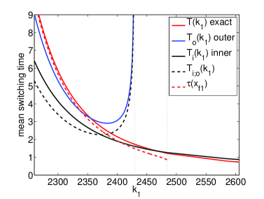
      (a) ​​​​ (b)

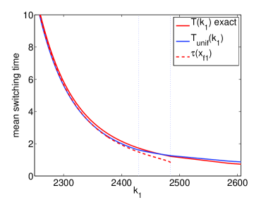
Fig. 8: (a) The inner solution $(\ref{tauinnerapp})$ as a function of $k_{1}$ (black line). The red line is the exact value $T(k_{1})$ given by $(\ref{taudef2})$. We also plot the outer solution $(\ref{tauouterapp})$ (blue line), the outer limit of the inner solution $(\ref{tauioform})$ (black dashed line) and $\tau(x_{f1})$ given by $(\ref{tauzformula})$ for $b=(x_{u}+x_{f2})/2$ (red dashed line). (b) The uniform approximation $T_{unif}(k_{1})$ which is given by $(\ref{tauunifform})$ (blue line). We also plot the exact value $T(k_{1})$ given by $(\ref{taudef2})$ (red line) and $\tau(x_{f1})$ given by $(\ref{tauzformula})$ for $b=(x_{u}+x_{f2})/2$ (red dashed line).

(48) with the exact value $T(k_{1})$ given by $(\ref{taudef2})$. We also plot $\tau(x_{f1})$ given by (25) for $b=(x_{u}+x_{f2})/2.$ As discussed before, $\tau(x_{f1})$ could be considered as another possible definition of the mean switching time. We see that the value of the inner approximation $T_{i}(k_{1})$ at the critical point $k_{1}=K$ lies between the exact value $T(k_{1})$ and $\tau(x_{f1})$. Thus we confirm that $T_{i}(k_{1})$ is a good approximation of $T(k_{1})$ for $k_{1}$ close the the critical point $K$.

3.4 Uniform approximation of the mean switching time $T(k_{1})$

In Section 3.2, we obtained the outer approximation (38) of the mean switching time which is valid for $k_{1}\ll K$. In Section 3.3, we obtained the inner approximation (48) of the mean switching time which is valid for $k_{1}\approx K$. In this section, we match the inner and the outer solutions to derive the uniform approximation of the mean switching time. First, we investigate the asymptotic behaviour of $H(z)$ as $z\to\infty$. Let $z>0$. Using the substitution $w=z^{-1/2}v$ in the definition (47), we obtain

$$H(z)=z^{1/4}\int_{0}^{\infty}\frac{1}{\sqrt{w}}\,\exp\left[z^{3/2}\left(w-w^{3}\right)\right]\,\mbox{d}w\;\sim\;\sqrt{\frac{\pi}{z}}\exp\left[\frac{2z^{3/2}}{3\sqrt{3}}\right]\qquad\mbox{as}\;z\to\infty.$$

Consequently, the outer limit of the inner solution (48) is

$$T_{i;o}=\frac{2^{1/2}\pi}{\sqrt{|k_{1}-K|}}\left(\frac{\partial^{2}v}{\partial y^{2}}(y_{k},K)\right)^{\!-1/2}\exp\!\left[\frac{4\sqrt{2}}{3d(y_{k})}|k_{1}-K|^{3/2}\left(\frac{\partial^{2}v}{\partial y^{2}}(y_{k},K)\right)^{\!-1/2}\right].$$ (49)

In Figure 8(a), we plot $T_{i;o}(k_{1})$ as the black dashed line. It is easy to check that the inner limit of the outer solution $T_{o}(k_{1})$ is equal to the outer limit of the inner solution $T_{i}(k_{1})$, i.e. it is also given by $T_{i;o}(k_{1})$. Thus we can define the continuous uniform approximation of the mean switching time $T(k_{1})$ by the formula

$$T_{unif}(k_{1})\equiv\begin{cases}T_{o}(k_{1})+T_{i}(k_{1})-T_{i;o}(k_{1})-C,&\mbox{for}\;k_{1}<K;\\ T_{i}(k_{1}),&\mbox{for}\;k_{1}\geq K;\\ \end{cases}$$ (50)

where the constant $C$ is defined by

$$C=\lim_{\;\,k_{1}\to K_{-}}\left(T_{o}(k_{1})-T_{i;o}(k_{1})\right).$$

Thus, for $k_{1}<K$, we add the inner and the outer solutions and subtract the “overlap” solution (the inner limit of the outer solution) which has been double-counted. In order to make the approximation continuous at $k_{1}=K$, we also subtract the constant $C$ (which is in fact a higher order term). We approximate $T(k_{1})$ by the inner solution for $k_{1}\geq K$. In Figure 8(b), we plot the uniform approximation $T_{unif}(k_{1})$ together with the exact value $T(k_{1})$ given by $(\ref{taudef2})$. We also plot $\tau(x_{f1})$ given by (25) for $b=(x_{u}+x_{f2})/2.$ The comparison is excellent.

4 Numerical results obtained by solving the chemical Fokker-Planck equation for the chemical SNIPER problem

We consider the chemical system (1)–(2). Substituting the propensity functions (7) into the equation (95) in Appendix A, we obtain the chemical Fokker-Planck equation

$$\frac{\partial P}{\partial t}=\frac{\partial^{2}}{\partial x^{2}}\big{[}d_{x}\,P\big{]}+\frac{\partial^{2}}{\partial x\partial y}\big{[}d_{xy}\,P\big{]}+\frac{\partial^{2}}{\partial y^{2}}\big{[}d_{y}\,P\big{]}-\frac{\partial}{\partial x}\big{[}v_{x}\,P\big{]}-\frac{\partial}{\partial y}\big{[}v_{y}\,P\big{]}$$ (51)

where $P(x,y,t)$ is the joint probability distribution that $X(t)=x$ and $Y(t)=y$, $x\in[0,\infty)$, $y\in[0,\infty)$, and the drift and diffusion coefficients are given by

$$v_{x}(x,y) = k_{2}y-k_{5}x(x-1)(x-2)+k_{4}x(x-1)-k_{3}x,$$ (52)

$$v_{y}(x,y) = -k_{7}x(x-1)y+k_{6}xy-k_{2}y+k_{1},$$ (53)

$$d_{x}(x,y) = [k_{2}y+k_{5}x(x-1)(x-2)+k_{4}x(x-1)+k_{3}x]/2,$$ (54)

$$d_{y}(x,y) = [k_{7}x(x-1)y+k_{6}xy+k_{2}y+k_{1}]/2,$$ (55)

$$d_{xy}(x,y) = -k_{2}y.$$ (56)

The stationary distribution $P_{s}(x,y)=\lim_{t\to\infty}P(x,y,t)$ can be obtained as a solution of the corresponding elliptic problem:

$$0=\frac{\partial^{2}}{\partial x^{2}}\big{[}d_{x}\,P_{s}\big{]}+\frac{\partial^{2}}{\partial x\partial y}\big{[}d_{xy}\,P_{s}\big{]}+\frac{\partial^{2}}{\partial y^{2}}\big{[}d_{y}\,P_{s}\big{]}-\frac{\partial}{\partial x}\big{[}v_{x}\,P_{s}\big{]}-\frac{\partial}{\partial y}\big{[}v_{y}\,P_{s}\big{]},$$ (57)

$$\int_{0}^{\infty}\int_{0}^{\infty}P_{s}(x,y)\mbox{d}x\mbox{d}y=1,$$ (58)

$$P_{s}(x,y)\geq 0,\qquad\qquad\mbox{for all}\;(x,y)\in[0,\infty)\times[0,\infty).$$ (59)

To solve the problem (57)–(59) approximately by the finite element method (FEM) we have to reformulate it as a problem in a finite domain. Therefore, we first restrict the domain $[0,\infty)\times[0,\infty)$ to a rectangle $S$ which has to be sufficiently large to contain most of the trajectories. For example, Figure 2(b) shows the illustrative trajectory for the parameter values (5) and $V=40$. In this case, the rectangle $S$ can be chosen as $S=(0,500)\times(0,2000)$. On the boundary $\partial S$ we prescribe homogeneous Neumann boundary conditions. We reformulate (57)–(59) as the following Neumann problem in the domain $S$

$$-\operatorname{div}(\mathcal{A}\nabla P_{s}+P_{s}\mathbf{b}) = 0\quad\text{in }S,$$ (60)

$$(\mathcal{A}\nabla P_{s}+P_{s}\mathbf{b})\cdot\mathbf{n} = 0\quad\text{on }\partial S,$$

where $\nabla$ stands for the gradient, $\mathbf{n}$ denotes the outward unit normal vector to $\partial S$, and the $2\times 2$ symmetric positive definite matrix $\mathcal{A}$ and the vector $\mathbf{b}$ are given by

$$\mathcal{A}=\left(\begin{matrix}-d_{x}&-d_{xy}/2\\ -d_{xy}/2&-d_{y}\end{matrix}\right),\quad\mathbf{b}=\left(v_{x}-\frac{\partial d_{x}}{\partial x}-\frac{1}{2}\frac{\partial d_{xy}}{\partial y},v_{y}-\frac{\partial d_{y}}{\partial y}-\frac{1}{2}\frac{\partial d_{xy}}{\partial x}\right)^{T}.$$ (61)

To define the FEM solution, we need the weak formulation of (60). The weak solution $P_{s}\in H^{1}(S)$ is uniquely determined by the requirement

$$a(P_{s},\varphi)=0\quad\forall\varphi\in H^{1}(S),$$

where $H^{1}(S)$ stands for the Sobolev space $W^{1,2}(S)$ and the bilinear form $a(\cdot,\cdot)$ is given by

$$a(P_{s},\varphi)=\int_{S}(\mathcal{A}\nabla P_{s}+P_{s}\mathbf{b})\cdot\nabla\varphi\,\mbox{d}x\mbox{d}y.$$

We use first-order triangular elements. First we define a triangulation $\mathcal{T}_{h}$ of the domain $S$ and the corresponding finite element subspace $W_{h}$ of the piecewise linear functions:

$$W_{h}=\{\varphi_{h}\in H^{1}(S):\varphi_{h}|_{K}\in P^{1}(K),\ K\in\mathcal{T}_{h}\},$$ (62)

where $P^{1}(K)$ stands for the three-dimensional space of linear functions on the triangle $K\in\mathcal{T}_{h}$. The finite element problem then reads: find $P_{s,h}\in W_{h}$ such that

$$a(P_{s,h},\varphi_{h})=0\quad\forall\varphi_{h}\in W_{h}.$$ (63)

Both problems (60) and (63) posses trivial solutions $P_{s}\equiv 0$ and $P_{s,h}\equiv 0$. To get a non-zero solution we use appropriate numerical methods for finding eigenvectors corresponding to the zero eigenvalue. The computed nontrivial solution $P_{s,h}$ is then normalized to have $\int_{S}P_{s,h}(x,y)\mbox{d}x\mbox{d}y=1$. In Figure 9(a), we present the FEM solution $P_{s,h}$ to the problem (63) obtained on a uniform mesh with $2^{18}$ triangular elements. We use the parameter values (5) and $V=40$. We plot only the stationary distribution in the subdomain $[0,80]\times[550,1150],$ i.e. the part of the $X$-$Y$ phase space where the system spends most of time. Running long time stochastic simulations, we can find the stationary distribution by the Gillespie SSA, which is plotted in Figure 9(b) for the same parameter values $(\ref{sniperparam})$ and $V=40$. The comparison with the results obtained by the chemical Fokker-Planck equation is visually excellent.

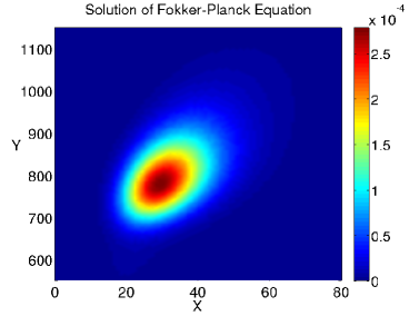
      (a) ​​​​ (b)

Fig. 9: (a) The FEM solution of the Fokker-Planck equation $(\ref{problemAF})$ restricted to the subdomain $(0,80)\times(550,1150)$. (b) $P_{s}(x,y)$ obtained by the Gillespie SSA. We use the parameter values $(\ref{sniperparam})$ and $V=40$.

Plotting the numerical results in the whole computational domain $S=(0,500)\times(0,2000)$, we do not see any additional information because most of $P_{s}$ is localized in the subdomain shown in Figure 9. We have to plot $\log(P_{s})$ to see the underlying “volcano-shaped” probability distribution – see Figure 10 (a).

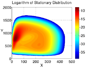
      (a) ​​​​ (b)

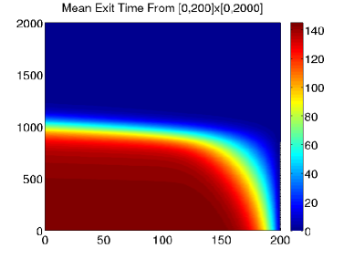
Fig. 10: (a) Logarithm of the FEM solution of the Fokker-Planck equation $(\ref{problemAF})$ in the domain $S=(0,500)\times(0,2000)$. (b) The solution $\tau(x,y)$ of $(\ref{finproblemtau})$ computed by the FEM. We use the parameter values $(\ref{sniperparam})$ and $V=40$.

Let us note that there is no bifurcation in the features of $P_{s}$, i.e. the probability distribution is “volcano-shaped” both before and after the ODE critical value.

4.1 Computation of the period of oscillation

Let us consider the SNIPER chemical system (1)–(2) with the parameter values (5) and $V=40$. An illustrative stochastic trajectory is shown in Figure 2. Let the domain $\Omega$ be defined by $\Omega=\{[x,y]\;|\;x<200\}$. In each cycle (as we defined it on page 3), the trajectory leaves the domain $\Omega$. However, the time which the trajectory spends outside the domain $\Omega$ is much smaller than the time which the trajectory spends inside $\Omega$. This observation is confirmed by Figure 10(a). The probability that the system state is outside $\Omega$ is several orders of magnitude smaller than the probability that it lies inside $\Omega$. Thus the period of oscillation can be estimated as the mean time to leave the domain $\Omega$ provided that the trajectory “has just entered it”. Let $\tau(x,y)$ be the average time to leave the domain $\Omega$ provided that the trajectory starts at $X(0)=x$ and $Y(0)=y$. As shown in Appendix B, $\tau(x,y)$ evolves according to the equation (98):

$$d_{x}\frac{\partial^{2}\tau}{\partial x^{2}}+d_{xy}\frac{\partial^{2}\tau}{\partial x\partial y}+d_{y}\frac{\partial^{2}\tau}{\partial y^{2}}+v_{x}\frac{\partial\tau}{\partial x}+v_{y}\frac{\partial\tau}{\partial y}=-1,\quad\mbox{for}\;[x,y]\in\Omega,$$ (64)

together with the boundary condition $\tau(200,y)=0$ for $y\in{\mathbb{R}}$. To solve this problem approximately, we truncate the domain $\Omega$ to get the finite domain $\widetilde{S}=(0,200)\times(0,2000)$. We consider homogeneous Neumann boundary conditions on the parts of the boundary which are not on the line $x=200$ and we rewrite the problem (64) in the form

$$-\operatorname{div}(\mathcal{A}\nabla\tau)+\mathbf{b}\cdot\nabla\tau = -1\quad\text{in }\widetilde{S},$$ (65)

$$\tau = 0\quad\text{on the line }x=200,$$

$$(\mathcal{A}\nabla\tau)\cdot{\mathbf{n}} = 0\quad\text{on the lines }y=0,\ y=2000,\ x=0,$$

where the $2\times 2$ matrix $\mathcal{A}$ and the vector $\mathbf{b}$ are given by (61) and the coefficients $d_{x}$, $d_{xy}$, $d_{y}$, $v_{x}$, and $v_{y}$ are given by (52)–(56). Notice the difference between (65) and (60) and that $\widetilde{S}\subset S.$ As in the previous section, we define the weak solution as $\tau\in\widetilde{W}$ satisfying

$$\widetilde{a}(\tau,\varphi)=\int_{\widetilde{S}}-1\cdot\varphi\,\mbox{d}x\mbox{d}y\qquad\forall\varphi\in\widetilde{W},$$

where $\widetilde{W}=\{v\in H^{1}(\widetilde{S}):v=0$ on the line $x=200\}$ and

$$\widetilde{a}(\tau,\varphi)=\int_{\widetilde{S}}\mathcal{A}\nabla\tau\cdot\nabla\varphi\,\mbox{d}x\mbox{d}y+\int_{\widetilde{S}}\mathbf{b}\cdot\nabla\tau\varphi\,\mbox{d}x\mbox{d}y.$$

The FEM solution $\tau_{h}\in\widetilde{W}_{h}$ is defined by the requirement

$$\widetilde{a}(\tau_{h},\varphi_{h})=\int_{\widetilde{S}}-1\cdot\varphi_{h}\,\mbox{d}x\mbox{d}y,\qquad\forall\varphi_{h}\in\widetilde{W}_{h},$$

where $\widetilde{W}_{h}\subset\widetilde{W}$ is the space of continuous and piecewise linear functions based on a suitable triangulation $\mathcal{T}_{h}$ of $\widetilde{S}$ (compare with (62)). The triangulation used does not follow the anisotropy of $\widetilde{S}$ and it consits of elements close to the equilateral triangle. It has about $500,000$ triangles and the number of degrees of freedom is about $250,000$. The FEM solution $\tau_{h}$ is shown in Figure 10(b). Using the computed profile, we can estimate the period of oscillation. One possibility is to find the maximum of the stationary distribution $P_{s}(x,y)$ which is attained at the point $[x_{f},y_{f}]=[29.30,781.25]$, and estimate the period of oscillation as $\tau_{h}(x_{f},y_{f})=\tau_{h}(29.30,781.25)\doteq 134.1$. This compares well with the period of oscillation estimated by long stochastic simulation for the same parameter values. We obtained $130.4$ as an average over $10^{5}$ periods.

The estimation of the period of oscillation is analogous to the estimation of the mean switching time of the Schlögl problem (8) which was studied in Section 3. We introduced the boundary $b$ given by (26) and we asked what the mean time to leave the domain $(-\infty,b)$ is. The biggest contribution to the mean exit time was given by the behaviour close to the point $x_{u}$. The SNIPER equivalent of the boundary $b$ (resp. point $x_{u}$) is the line $x=200$ (resp. the saddle). In the case of the Schlögl problem (8), we saw that the difference between the escape times from $X(0)=0$ and $X(0)=x_{f1}$ increased as we approached the bifurcation value. Similarly, the estimation of the period of oscillation of the SNIPER problem by $\tau_{h}(x_{f},y_{f})$ is fine for $k_{1d}\ll K_{d}$, but it might provide less accurate results if the saddle and the stable node of the SNIPER problem are too close, i.e. if $k_{1d}$ is close to the bifurcation value $K_{d}$. Thus it is better to estimate the mean period of oscillation as the mean time to leave the domain $\Omega$, starting from the subdomain $\gamma\subset\Omega$ where stochastic trajectories enter the domain $\Omega$. We approximate the mean period of oscillation as a weighted average of $\tau(x,y)$ over a suitable subdomain $\gamma$, namely by

$$T(\gamma)=\frac{\displaystyle\int_{\gamma}\tau(x,y)\,P_{s}(x,y)\,\mbox{d}x\mbox{d}y}{\displaystyle\int_{\gamma}P_{s}(x,y)\,\mbox{d}x\mbox{d}y}.$$ (66)

Since the trajectories are entering the domain $\widetilde{S}$ at the smaller values of $Y$ and leaving the domain at the larger values of $Y$, it is reasonable to choose the subdomain $\gamma$ as the line segment parallel with the $Y$ axis between the $X$ axis and a suitable treshold value. Three choices of $\gamma$ are shown in Figure 11(a) as thick black, magenta and green lines.

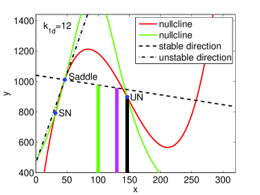
    (a) ​​​​ (b)

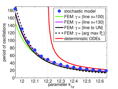
Fig. 11: (a) Nullclines and steady states of the ODE system $(\ref{detSNIPERode})$ together with the lines $\gamma$ which are used in the formula $(\ref{apposc})$. The lines $\gamma$ are plotted as the thick green line (for $x=100$), the magenta line (for $x=130$) and the black line (for the line to the unstable node). (b) The period of oscillation as a function of the parameter $k_{1d}$. The results obtained by the Gillespie SSA (blue circles) are compared with the results obtained by $(\ref{apposc})$ for the lines $\gamma$ shown in the panel (a).

The black line is the line from $y=0$ to the unstable node. The magenta line is a segment of $x=130$ and the thick green line is a segment of $x=100$. In the case of $x=100$ (resp. $x=130$), we define the threshold value as the intersection of the line $x=100$ (resp. $x=130$) with the stable direction at the saddle point. Note that we use the nullclines and the saddle point of the system of ODEs

$$\frac{\mbox{d}x}{\mbox{d}t}=v_{x}(x,y),\qquad\frac{\mbox{d}y}{\mbox{d}t}=v_{y}(x,y)$$ (67)

which slightly differs from the classical mean-field ODE description (3)–(4). The ODE system (67) is equivalent to the ODE system (3)–(4) in the limit $V\to\infty$. See also the discussion after the equation (19) about the differences between (9) and (19).

In Figure 11(b), we present estimates of the period of oscillation computed by (66) as a function of the parameter $k_{1d}$. The results obtained by the Gillespie SSA (blue circles) and by the ODEs (3)–(4) (red line) were already presented in Figure 4(a). The green, magenta and black curves correspond to the results computed by (66) for the lines $\gamma$ of the same colour in Figure 11(a). We also present results computed by $\tau(x_{f},y_{f})$ where $[x_{f},y_{f}]$ is the point where $P_{s}(x,y)$ achieves its maximum. The dotted line denotes the bifurcation values of the ODE systems (3)–(4) and (67). These values differ for finite values of the volume $V$. In Figure 12(a), we show the dependence of the bifurcation value of $k_{1d}$ on the volume $V$ for both ODE systems. The ODE system (3)–(4) is independent of $V$, and so its bifurcation value. Fixing the value of $k_{1d}$ at the bifurcation value $K_{d}\doteq 12.2$ of the ODE model (3)–(4), the period of oscillation of the ODE system (3)–(4) is infinity. The ODE system (67) does not have a limit cycle at all as $K_{d}\doteq 12.2$ is below its bifurcation value which we denote $K$. However, we saw in Figure 4(b) that the stochastic system has oscillatory solutions with a finite period for $k_{1d}=K_{d}.$ The period of oscillation as a function of the volume $V$ can be also computed by (66). The results are shown in Figure 12(b). We use the same lines $\gamma$ as in Figure 11(a). We have to take into account that the system volume $V$ changes and that the phase plane axes (the number of species particles) scale linearly with $V$. Thus we define the lines $\gamma$ as segments of $x=0.67x^{u}$, $x=0.87x^{u}$ and $x=x^{u}$ where $x^{u}$ is the $x$-coordinate of the unstable node. This definition gives for $V=40$ the lines $\gamma$ plotted in Figure 11(a). We also have to scale the domain $\widetilde{S}$ with $V$: we use $\widetilde{S}V/40$ instead of $\widetilde{S}$. Fortunately, we can simply rescale the triangulation. Thus the volume dependence of the computational domain does not causes any additional problems. Let us note that the $y$ threshold for the lines at $x=0.67x^{u}$ and $x=0.87x^{u}$ is defined as an intersection with the stable direction at the saddle point of (67). As shown in Figure 12(a), the saddle point of the ODE system (67) is always defined for $k_{1d}\doteq K_{d}$ because its (volume dependent) bifurcation value $K$ satisfies $K>K_{d}$. Let us note that for $k_{1}$ greater than the bifurcation value of (67), we use the lines $\gamma$ computed at the bifurcation point (since there is no saddle defined for such values of $k_{1d}$). This definition was used in Figure 11(b) for $k_{1d}>K$.

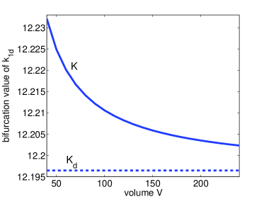
      (a) ​​​​ (b)

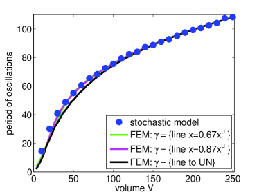
Fig. 12: (a) The dependence of the bifurcation value of the parameter $k_{1d}$ on the volume $V$ for the ODE system $(\ref{detSNIPERode})$ (solid line) and for the ODE system $(\ref{eq1})$–$(\ref{eq2})$ (dashed line). The other parameter values are given according to $(\ref{sniperparam})$. (b) The period of oscillation as a function of the volume $V$. The results obtained by the Gillespie SSA (blue circles) are compared with the results obtained by $(\ref{apposc})$ for the lines $\gamma$ (scaled by $V$) which are shown in Figure 11(a).

5 Analytical results

In this section, we derive analytical formulae for the dependence of the period of oscillation of the chemical SNIPER problem (1)–(2) on the parameter $k_{1d}$ and on the volume $V$, i.e. we obtain formulae for the behaviour shown in Figure 4. In particular, we generalize the one-dimensional approach from Section 3.3 to the chemical SNIPER problem. As we mentioned before, we denote the bifurcation value of the parameter $k_{1d}$ of the ODE system (67) by $K$. If $k_{1d}=K$, then the saddle and the stable node of the ODE system (67) coincide at one point which we denote as $[x_{k},y_{k}].$ Let us define

$${\mathbf{A}}=\left(\begin{matrix}\displaystyle\frac{\partial v_{x}}{\partial x}&\displaystyle\frac{\partial v_{x}}{\partial y}\\ \displaystyle\frac{\partial v_{y}}{\partial x}&\displaystyle\frac{\partial v_{y}}{\partial y}\end{matrix}\right)(x_{k},y_{k},K),$$

where the dependence on parameters $k_{2},\dots,k_{7}$ is not indicated, because their values are fixed and given by (5). The eigenvalues of ${\mathbf{A}}$ are $\lambda_{1}=0$ and $\lambda_{2}=-\lambda_{0}<0$. We denote the corresponding eigenvectors as ${\mathbf{u}}_{1}=(u_{11},u_{21})$ (for the eignevalue zero) and ${\mathbf{u}}_{2}=(u_{12},u_{22})$ (for the eigenvalue $-\lambda_{0}$). The eigenvector ${\mathbf{u}}_{1}$ is in the direction of the limit cycle. There is an obvious separation of time scales. The dynamics is much slower in the direction of ${\mathbf{u}}_{1}$ than in the direction of ${\mathbf{u}}_{2}$. Thus we first transform the variables from the Cartesian coordinate system $x$ and $y$ to the directions of eigenvectors of ${\mathbf{A}}$ and then we analyse the transformed $\tau$-equation. To do it systematically, we use the following scaling (compare with (29))

$$x=\frac{\overline{x}}{\varepsilon},\quad y=\frac{\overline{y}}{\varepsilon},\quad v_{x}=\frac{\overline{v}_{x}}{\varepsilon^{2}},\quad v_{y}=\frac{\overline{v}_{y}}{\varepsilon^{2}},\quad d_{x}=\frac{\overline{d}_{x}}{\varepsilon^{2}},\quad d_{xy}=\frac{\overline{d}_{xy}}{\varepsilon^{2}},\quad d_{y}=\frac{\overline{d}_{y}}{\varepsilon^{2}}.$$

Then the $\tau$-equation (64) reads as follows

$$\varepsilon\,\overline{d}_{x}\,\frac{\partial^{2}\tau}{\partial\overline{x}^{2}}+\varepsilon\,\overline{d}_{xy}\,\frac{\partial^{2}\tau}{\partial\overline{x}\partial\overline{y}}+\varepsilon\,\overline{d}_{y}\,\frac{\partial^{2}\tau}{\partial\overline{y}^{2}}+\overline{v}_{x}\,\frac{\partial\tau}{\partial\overline{x}}+\overline{v}_{y}\,\frac{\partial\tau}{\partial\overline{y}}=-\varepsilon.$$ (68)

For $k_{1d}$ close to $K$ and $[\overline{x},\overline{y}]$ close to $[\overline{x}_{k},\overline{y}_{k}]$, we use the local variables $\eta,$ $\xi$ and $\kappa$ which are related to $\overline{x}$ and $\overline{y}$ as follows

$$\left(\begin{matrix}\overline{x}\\ \overline{y}\end{matrix}\right)=\left(\begin{matrix}\overline{x}_{k}\\ \overline{y}_{k}\end{matrix}\right)+\left(\begin{matrix}\overline{u}_{11}&\overline{u}_{12}\\ \overline{u}_{21}&\overline{u}_{22}\end{matrix}\right)\left(\begin{matrix}\varepsilon^{1/3}\,\eta\\ \varepsilon^{1/2}\,\xi\end{matrix}\right),\qquad k_{1d}V=k_{1}=K+\varepsilon^{2/3}\kappa.$$ (69)

Then the line $\xi=0$ corresponds to the direction of the limit cycle and $\eta=0$ to the stable direction. Let us denote $\overline{q}=[\overline{x}_{k},\overline{y}_{k},K]$ to shorten the following formulae. Using the Taylor expansion at the point $\overline{q}=[\overline{x}_{k},\overline{y}_{k},K]$, we approximate

$$\overline{d}_{x}(\overline{x},\overline{y},k_{1}) \approx \overline{d}_{x}(\overline{q})+\varepsilon^{1/3}c_{1}(\overline{d}_{x})\,\eta+\varepsilon^{1/2}c_{2}(\overline{d}_{x})\,\xi+\varepsilon^{2/3}c_{3}(\overline{d}_{x})\,\eta^{2}+o(\varepsilon^{5/6}),$$

$$\overline{d}_{xy}(\overline{x},\overline{y},k_{1}) \approx \overline{d}_{xy}(\overline{q})+\varepsilon^{1/3}c_{1}(\overline{d}_{xy})\,\eta+\varepsilon^{1/2}c_{2}(\overline{d}_{xy})\,\xi+\varepsilon^{2/3}c_{3}(\overline{d}_{xy})\,\eta^{2}+o(\varepsilon^{5/6}),$$

$$\overline{d}_{y}(\overline{x},\overline{y},k_{1}) \approx \overline{d}_{y}(\overline{q})+\varepsilon^{1/3}c_{1}(\overline{d}_{y})\,\eta+\varepsilon^{1/2}c_{2}(\overline{d}_{y})\,\xi+\varepsilon^{2/3}c_{3}(\overline{d}_{y})\,\eta^{2}+o(\varepsilon^{5/6}),$$

where $c_{i}(\overline{d}_{x}),$ $c_{i}(\overline{d}_{xy})$ and $c_{i}(\overline{d}_{y})$ are constants. To systematically derive the formulae for the mean period of oscillation, we need to take all the terms above into account. However, we will show that the results are actually independent of some coefficients in the expansion. To save space, we explicitly specify only those coefficients which actually appears in the final formulae. They are given in Appendix C. Using the fact that ${\mathbf{u}}_{1}=(u_{11},u_{21})$ (resp. ${\mathbf{u}}_{2}=(u_{12},u_{22})$) is an eigenvector of the matrix ${\mathbf{A}}$ corresponding to the eigenvalue $\lambda_{1}=0$ (resp. $\lambda_{2}=-\lambda_{0}<0$), we obtain the expansion of $\overline{v}_{x}$ and $\overline{v}_{y}$ in the form

$$\overline{v}_{x}(\overline{x},\overline{y},k_{1}) \approx -\varepsilon^{1/2}\lambda_{0}\overline{u}_{12}\,\xi+\varepsilon^{2/3}c_{1}(\overline{v}_{x})\,\eta^{2}+\varepsilon^{5/6}c_{2}(\overline{v}_{x})\,\eta\xi$$

$$+ \varepsilon(c_{3}(\overline{v}_{x})\,\xi^{2}+c_{4}(\overline{v}_{x})\,\eta^{3})+\varepsilon^{7/6}c_{5}(\overline{v}_{x})\,\eta^{2}\xi+o(\varepsilon^{4/3}),$$

$$\overline{v}_{y}(\overline{x},\overline{y},k_{1}) \approx -\varepsilon^{1/2}\lambda_{0}\overline{u}_{22}\,\xi+\varepsilon^{2/3}(c_{1}(\overline{v}_{y})\,\eta^{2}+\kappa)+\varepsilon^{5/6}\xi c_{2}(\overline{v}_{y})\,\eta$$

$$+ \varepsilon(c_{3}(\overline{v}_{y})\,\xi^{2}+c_{4}(\overline{v}_{y}))\,\eta^{3})+\varepsilon^{7/6}c_{5}(\overline{v}_{y})\,\eta^{2}\xi+o(\varepsilon^{4/3}),$$

where the constants $c_{i}(\overline{v}_{x})$ and $c_{i}(\overline{v}_{y})$ are given in Appendix C. Using (69), the derivatives transform as follows

$$\frac{\partial}{\partial\overline{x}} = \frac{\partial}{\partial\eta}\frac{\partial\eta}{\partial\overline{x}}+\frac{\partial}{\partial\xi}\frac{\partial\xi}{\partial\overline{x}}=\varepsilon^{-1/3}\frac{\overline{u}_{22}}{\det\overline{U}}\frac{\partial}{\partial\eta}-\varepsilon^{-1/2}\frac{\overline{u}_{21}}{\det\overline{U}}\frac{\partial}{\partial\xi},$$

$$\frac{\partial}{\partial\overline{y}} = \frac{\partial}{\partial\eta}\frac{\partial\eta}{\partial\overline{y}}+\frac{\partial}{\partial\xi}\frac{\partial\xi}{\partial\overline{y}}=-\varepsilon^{-1/3}\frac{\overline{u}_{12}}{\det\overline{U}}\frac{\partial}{\partial\eta}+\varepsilon^{-1/2}\frac{\overline{u}_{11}}{\det\overline{U}}\frac{\partial}{\partial\xi},$$

where $\det\overline{U}=\overline{u}_{11}\overline{u}_{22}-\overline{u}_{12}\overline{u}_{21}$. Substituting our approximations to (68) and using the scaling $\tau=\varepsilon^{2/3}\overline{\tau}$, we obtain

$$0 = \left(-\lambda_{0}\,\xi\frac{\partial\overline{\tau}}{\partial\xi}+\sigma_{1}\frac{\partial^{2}\overline{\tau}}{\partial\xi^{2}}\right)+\varepsilon^{1/6}\left(\sigma_{2}\,\eta^{2}\frac{\partial\overline{\tau}}{\partial\xi}+\sigma_{3}\,\kappa\frac{\partial\overline{\tau}}{\partial\xi}+\sigma_{4}\frac{\partial^{2}\overline{\tau}}{\partial\xi\partial\eta}\right)$$ (70)

$$+ \varepsilon^{1/3}\left(\sigma_{5}\,\eta^{2}\frac{\partial\overline{\tau}}{\partial\eta}+\sigma_{6}\,\kappa\frac{\partial\overline{\tau}}{\partial\eta}+\sigma_{7}\,\xi\eta\frac{\partial\overline{\tau}}{\partial\xi}+\sigma_{8}\frac{\partial^{2}\overline{\tau}}{\partial\eta^{2}}+\sigma_{9}\,\eta\frac{\partial^{2}\overline{\tau}}{\partial\xi^{2}}+1\right)$$

$$+ \varepsilon^{1/2}\left(\sigma_{10}\,\xi\eta\frac{\partial\overline{\tau}}{\partial\eta}+\sigma_{11}\,\xi^{2}\frac{\partial\overline{\tau}}{\partial\xi}+\sigma_{12}\,\eta^{3}\frac{\partial\overline{\tau}}{\partial\xi}+\sigma_{13}\,\xi\frac{\partial^{2}\overline{\tau}}{\partial\xi^{2}}+\sigma_{14}\,\eta\frac{\partial^{2}\overline{\tau}}{\partial\xi\partial\eta}\right)$$

$$+ \varepsilon^{2/3}\left(\sigma_{15}\,\eta^{2}\frac{\partial^{2}\overline{\tau}}{\partial\xi^{2}}+\sigma_{16}\,\xi\frac{\partial^{2}\overline{\tau}}{\partial\xi\partial\eta}+\sigma_{17}\,\eta\frac{\partial^{2}\overline{\tau}}{\partial\eta^{2}}+\sigma_{18}\,\xi^{2}\frac{\partial\overline{\tau}}{\partial\eta}\right.$$

$$\qquad\;\;+\left.\sigma_{19}\,\eta^{3}\frac{\partial\overline{\tau}}{\partial\eta}+\sigma_{20}\,\eta^{2}\xi\frac{\partial\overline{\tau}}{\partial\xi}\right)+o(\varepsilon^{5/6}),$$

where the coefficients $\sigma_{i}$ are given in the Appendix C. We assume that $\overline{\tau}\to 0$ as $\eta\to\infty$ and that $\overline{\tau}$ is bounded as $\eta\to-\infty$ and $\xi\to\pm\infty$. We expand $\overline{\tau}$ as

$$\overline{\tau}\sim\tau_{0}+\varepsilon^{1/6}\tau_{1}+\varepsilon^{1/3}\tau_{2}+\varepsilon^{1/2}\tau_{3}+\varepsilon^{2/3}\tau_{4}+o(\varepsilon^{5/6}).$$

Substituting into (70), we obtain the following equation, at $O(\varepsilon^{0})$,

$$\lambda_{0}\,\xi\frac{\partial\tau_{0}}{\partial\xi}-\sigma_{1}\frac{\partial^{2}\tau_{0}}{\partial\xi^{2}}=0.$$ (71)

Integrating over $\xi$, we obtain

$$\frac{\partial\tau_{0}}{\partial\xi}=C(\eta)\exp\left[\frac{\lambda_{0}\xi^{2}}{2\sigma_{1}}\right],$$

where $C$ is a function of $\eta$. Since $\tau$ is assumed to be bounded as $\xi\to\pm\infty$, we must have $C(\eta)\equiv 0$. Consequently, we obtain

$$\tau_{0}\equiv\tau_{0}(\eta),$$ (72)

i.e. $\tau_{0}$ is not a function of $\xi$. Using (72) in (70), we obtain the following equation, at $O(\varepsilon^{1/6})$,

$$\lambda_{0}\,\xi\frac{\partial\tau_{1}}{\partial\xi}-\sigma_{1}\frac{\partial^{2}\tau_{1}}{\partial\xi^{2}}=0,$$ (73)

which similarly implies

$$\tau_{1}\equiv\tau_{1}(\eta).$$ (74)

Using (72) and (74) in (70), we have, at $O(\varepsilon^{1/3})$,

$$\lambda_{0}\,\xi\frac{\partial\tau_{2}}{\partial\xi}-\sigma_{1}\frac{\partial^{2}\tau_{2}}{\partial\xi^{2}}=\sigma_{5}\,\eta^{2}\frac{\partial\tau_{0}}{\partial\eta}+\sigma_{6}\,\kappa\frac{\partial\tau_{0}}{\partial\eta}+\sigma_{8}\frac{\partial^{2}\tau_{0}}{\partial\eta^{2}}+1.$$ (75)

Thus

$$-\sigma_{1}\frac{\partial}{\partial\xi}\left(\exp\left[-\frac{\lambda_{0}\xi^{2}}{2\sigma_{1}}\right]\frac{\partial\tau_{2}}{\partial\xi}\right)=\exp\left[-\frac{\lambda_{0}\xi^{2}}{2\sigma_{1}}\right]\left(\left(\sigma_{5}\eta^{2}+\sigma_{6}\kappa\right)\frac{\partial\tau_{0}}{\partial\eta}+\sigma_{8}\frac{\partial^{2}\tau_{0}}{\partial\eta^{2}}+1\right).$$

Integrating over $\xi$ in $(-\infty,\infty)$, we obtain the solvability condition

$$\left(\sigma_{5}\eta^{2}+\sigma_{6}\kappa\right)\frac{\partial\tau_{0}}{\partial\eta}+\sigma_{8}\frac{\partial^{2}\tau_{0}}{\partial\eta^{2}}=-1.$$ (76)

This equation is the SNIPER equivalent of equation (43) for the chemical switch, and can be solved to find the leading-order period of oscillation. Before we do so, we proceed to higher-order with the expansion to determine the correction term to $\tau_{0}.$ Using (76) in (75) gives

$$\lambda_{0}\,\xi\frac{\partial\tau_{2}}{\partial\xi}-\sigma_{1}\frac{\partial^{2}\tau_{2}}{\partial\xi^{2}}=0.$$

Thus, again,

$$\tau_{2}\equiv\tau_{2}(\eta).$$ (77)

Using (72), (74) and (77) in (70), we have, at $O(\varepsilon^{1/2})$,

$$\lambda_{0}\,\xi\frac{\partial\tau_{3}}{\partial\xi}+\sigma_{1}\frac{\partial^{2}\tau_{3}}{\partial\xi^{2}}=\sigma_{5}\,\eta^{2}\frac{\partial\tau_{1}}{\partial\eta}+\sigma_{6}\,\kappa\frac{\partial\tau_{1}}{\partial\eta}+\sigma_{8}\frac{\partial^{2}\tau_{1}}{\partial\eta^{2}}+\sigma_{10}\,\xi\eta\frac{\partial\tau_{0}}{\partial\eta}$$ (78)

which is equivalent to

$$- \sigma_{1}\frac{\partial}{\partial\xi}\left(\exp\left[-\frac{\lambda_{0}\xi^{2}}{2\sigma_{1}}\right]\frac{\partial\tau_{3}}{\partial\xi}\right)\qquad\qquad\qquad\qquad$$

$$= \exp\left[-\frac{\lambda_{0}\xi^{2}}{2\sigma_{1}}\right]\left(\left(\sigma_{5}\,\eta^{2}+\sigma_{6}\,\kappa\right)\frac{\partial\tau_{1}}{\partial\eta}+\sigma_{8}\frac{\partial^{2}\tau_{1}}{\partial\eta^{2}}+\sigma_{10}\,\xi\eta\frac{\partial\tau_{0}}{\partial\eta}\right).$$

Integrating over $\xi$ in $(-\infty,\infty)$, we obtain the solvability condition

$$\left(\sigma_{5}\,\eta^{2}+\sigma_{6}\,\kappa\right)\frac{\partial\tau_{1}}{\partial\eta}+\sigma_{8}\frac{\partial^{2}\tau_{1}}{\partial\eta^{2}}=0$$

which implies

$$\tau_{1}\equiv 0.$$ (79)

Consequently, (78) yields

$$-\sigma_{1}\frac{\partial}{\partial\xi}\left(\exp\left[-\frac{\lambda_{0}\xi^{2}}{2\sigma_{1}}\right]\frac{\partial\tau_{3}}{\partial\xi}\right)=\exp\left[-\frac{\lambda_{0}\xi^{2}}{2\sigma_{1}}\right]\left(\sigma_{10}\,\xi\eta\frac{\partial\tau_{0}}{\partial\eta}\right).$$

Integrating over $\xi$, we get

$$\frac{\partial\tau_{3}}{\partial\xi}=\frac{\sigma_{10}\,\eta}{\lambda_{0}}\frac{\partial\tau_{0}}{\partial\eta}.$$ (80)

Using (72), (79) and (77) in (70), we have, at $O(\varepsilon^{2/3})$,

$$\lambda_{0}\,\xi\frac{\partial\tau_{4}}{\partial\xi}-\sigma_{1}\frac{\partial^{2}\tau_{4}}{\partial\xi^{2}} = \sigma_{2}\,\eta^{2}\frac{\partial\tau_{3}}{\partial\xi}+\sigma_{3}\,\kappa\frac{\partial\tau_{3}}{\partial\xi}+\sigma_{4}\frac{\partial^{2}\tau_{3}}{\partial\xi\partial\eta}$$ (81)

$$+ \sigma_{5}\,\eta^{2}\frac{\partial\tau_{2}}{\partial\eta}+\sigma_{6}\,\kappa\frac{\partial\tau_{2}}{\partial\eta}+\sigma_{8}\frac{\partial^{2}\tau_{2}}{\partial\eta^{2}}$$

$$+ \sigma_{17}\,\eta\frac{\partial^{2}\tau_{0}}{\partial\eta^{2}}+\sigma_{18}\,\xi^{2}\frac{\partial\tau_{0}}{\partial\eta}+\sigma_{19}\,\eta^{3}\frac{\partial\tau_{0}}{\partial\eta}.\qquad\quad$$

Using (80) on the right hand side to eliminate the term $\partial\tau_{3}/\partial\xi$ and (76) to eliminate $\partial^{2}\tau_{0}/\partial\eta^{2}$, we get

$$-\sigma_{1}\frac{\partial}{\partial\xi}\left(\exp\left[-\frac{\lambda_{0}\xi^{2}}{2\sigma_{1}}\right]\frac{\partial\tau_{4}}{\partial\xi}\right)=\exp\left[-\frac{\lambda_{0}\xi^{2}}{2\sigma_{1}}\right]\times\Bigg{(}\left(\sigma_{5}\,\eta^{2}+\sigma_{6}\,\kappa\right)\frac{\partial\tau_{2}}{\partial\eta}+\sigma_{8}\frac{\partial^{2}\tau_{2}}{\partial\eta^{2}}$$

$$-\omega_{0}\,\eta+\left(\omega_{1}+\omega_{2}\,\kappa\,\eta+\omega_{3}\,\eta^{3}+\sigma_{18}\,\xi^{2}-\frac{\sigma_{18}\,\sigma_{1}}{\lambda_{0}}\right)\frac{\partial\tau_{0}}{\partial\eta}\Bigg{)},$$

where

$$\omega_{0}=\frac{\sigma_{4}\,\sigma_{10}}{\lambda_{0}\sigma_{8}}+\frac{\sigma_{17}}{\sigma_{8}},\qquad\omega_{1}=\frac{\sigma_{4}\,\sigma_{10}+\sigma_{18}\,\sigma_{1}}{\lambda_{0}},$$ (82)

$$\omega_{2}=\frac{\sigma_{3}\,\sigma_{10}}{\lambda_{0}}-\frac{\sigma_{4}\,\sigma_{6}\,\sigma_{10}}{\lambda_{0}\sigma_{8}}-\frac{\sigma_{6}\sigma_{17}}{\sigma_{8}},\qquad\omega_{3}=\frac{\sigma_{2}\,\sigma_{10}}{\lambda_{0}}+\sigma_{19}-\frac{\sigma_{4}\,\sigma_{5}\,\sigma_{10}}{\lambda_{0}\sigma_{8}}-\frac{\sigma_{5}\,\sigma_{17}}{\sigma_{8}}.$$

Integrating over $\xi$ in $(-\infty,\infty)$, we obtain the solvability condition

$$\left(\sigma_{5}\,\eta^{2}+\sigma_{6}\,\kappa\right)\frac{\partial\tau_{2}}{\partial\eta}+\sigma_{8}\frac{\partial^{2}\tau_{2}}{\partial\eta^{2}}=\omega_{0}\,\eta-\left(\omega_{1}+\omega_{2}\,\kappa\,\eta+\omega_{3}\,\eta^{3}\right)\frac{\partial\tau_{0}}{\partial\eta}.$$ (83)

This is the equation which determines $\tau_{2}$, the first non-zero correction term to $\tau_{0}$. Let us now solve (76) and (83) for $\tau_{0}$ and $\tau_{2}$. Since (76) is of the same form as the equation (43), we can use the same technique as in Section 3.3 to analyse it. We find (compare with (45))

$$\lim_{\eta\to-\infty}\tau_{0}(\eta)=\sqrt{\pi}\;3^{1/6}\left(\frac{2}{\sigma_{5}^{2}\,\sigma_{8}}\right)^{1/3}\,H\!\left(-\left(\frac{12}{\sigma_{5}\,\sigma_{8}^{2}}\right)^{\!1/3}\sigma_{6}\,\kappa\right),$$ (84)

where the function $H:{\mathbb{R}}\to(0,\infty)$ is given by (47). Moreover, we have the following identity (compare with (44))

$$\exp\left[\frac{\sigma_{5}\eta^{3}+3\sigma_{6}\kappa\eta}{3\sigma_{8}}\right]\frac{\partial\tau_{0}}{\partial\eta}=-\frac{1}{\sigma_{8}}\int_{-\infty}^{\eta}\exp\left[\frac{\sigma_{5}z^{3}+3\sigma_{6}\kappa z}{3\sigma_{8}}\right]\mbox{d}z.$$ (85)

Multiplying equation (83) by $\exp\left[(\sigma_{5}\eta^{3}+3\sigma_{6}\kappa\eta)/(3\sigma_{8})\right],$ using (85), integrating over $\eta$ and using integration by parts, we obtain

$$\frac{\partial\tau_{2}}{\partial\eta} = \int_{-\infty}^{\eta}\left(\frac{\omega_{0}}{\sigma_{8}}\,y+\frac{\omega_{1}}{\sigma_{8}^{2}}\,(\eta-y)+\frac{\omega_{2}}{2\sigma_{8}^{2}}\,\kappa\,(\eta^{2}-y^{2})+\frac{\omega_{3}}{4\sigma_{8}^{2}}\,(\eta^{4}-y^{4})\right)$$

$$\qquad\quad\times\exp\left[\frac{\sigma_{5}(y^{3}-\eta^{3})+3\sigma_{6}\kappa(y-\eta)}{3\sigma_{8}}\right]\mbox{d}y.$$

Integrating over $\eta$ in $(-\infty,\infty)$, we get

$$\lim_{\eta\to-\infty}\tau_{2}(\eta) = -\frac{\omega_{0}}{\sigma_{8}}\int_{-\infty}^{\infty}\int_{-\infty}^{z}y\exp\left[\frac{\sigma_{5}(y^{3}-z^{3})+3\sigma_{6}\kappa(y-z)}{3\sigma_{8}}\right]\mbox{d}y\,\mbox{d}z$$ (86)

$$+ \frac{\omega_{1}}{\sigma_{8}^{2}}\int_{-\infty}^{\infty}\int_{-\infty}^{z}(y-z)\exp\left[\frac{\sigma_{5}(y^{3}-z^{3})+3\sigma_{6}\kappa(y-z)}{3\sigma_{8}}\right]\mbox{d}y\,\mbox{d}z$$

$$+ \frac{\omega_{2}}{2\sigma_{8}^{2}}\,\kappa\int_{-\infty}^{\infty}\int_{-\infty}^{z}(y^{2}-z^{2})\exp\left[\frac{\sigma_{5}(y^{3}-z^{3})+3\sigma_{6}\kappa(y-z)}{3\sigma_{8}}\right]\mbox{d}y\,\mbox{d}z$$

$$+ \frac{\omega_{3}}{4\sigma_{8}^{2}}\int_{-\infty}^{\infty}\int_{-\infty}^{z}(y^{4}-z^{4})\exp\left[\frac{\sigma_{5}(y^{3}-z^{3})+3\sigma_{6}\kappa(y-z)}{3\sigma_{8}}\right]\mbox{d}y\,\mbox{d}z.\qquad\quad$$

Using the substitution

$$y=\left(\frac{3\sigma_{8}}{2\sigma_{5}}\right)^{1/3}\,(u-v),\qquad z=\left(\frac{3\sigma_{8}}{2\sigma_{5}}\right)^{1/3}\,(u+v),$$ (87)

we simplify the integrals on the right hand side of (86) using the same technique as in (45). In all cases, we are able to integrate over $u$ variable explicitly because the $u$-integral is the Gaussian integral. The last two integrals are zero because we integrate odd functions in $u$ over $(-\infty,\infty)$. Thus (86) becomes

$$\lim_{\eta\to-\infty}\tau_{2}(\eta)=\left(\omega_{0}-\frac{2\omega_{1}}{\sigma_{8}}\right)\frac{\sqrt{3\pi}}{\sigma_{5}}\int_{0}^{\infty}\sqrt{v}\exp\left[-v^{3}-\left(\frac{12}{\sigma_{5}\,\sigma_{8}^{2}}\right)^{1/3}\sigma_{6}\,\kappa\,v\right]\mbox{d}v.$$ (88)

Let us define the function $G:{\mathbb{R}}\to(0,\infty)$ by

$$G(z)=\int_{0}^{\infty}\sqrt{v}\exp\left[-v^{3}+zv\right]\,\mbox{d}v.$$ (89)

Using (82) and the definition (89), the formula (88) implies

$$\lim_{\eta\to-\infty}\tau_{2}(\eta)=\left(\sigma_{17}-\frac{\sigma_{4}\,\sigma_{10}}{\lambda_{0}}-\frac{2\sigma_{18}\,\sigma_{1}}{\lambda_{0}}\right)\frac{\sqrt{3\pi}}{\sigma_{5}\sigma_{8}}\,\,G\!\left(-\left(\frac{12}{\sigma_{5}\,\sigma_{8}^{2}}\right)^{1/3}\sigma_{6}\,\kappa\right).$$ (90)

The limits (84) and (90) give us the desired estimates of the period of oscillation. Transforming back to the original variables, the zero-order approximation to the mean period of oscillation is given by

$$T_{0}(k_{1})=\sqrt{\pi}\;3^{1/6}\left(\frac{2}{\sigma_{5}^{2}\,\sigma_{8}}\right)^{1/3}H\!\left(-\left(\frac{12}{\sigma_{5}\,\sigma_{8}^{2}}\right)^{\!1/3}\sigma_{6}\,(k_{1}-K)\right)$$ (91)

where the constants $\sigma_{5}$, $\sigma_{6}$ and $\sigma_{8}$ are given in Appendix C. More precisely, the formulae for the constants $\sigma_{5}$, $\sigma_{6}$ and $\sigma_{8}$ are obtained by dropping the overbars in their definitions in Appendix C. They only depend on the derivatives of the coefficients (52)–(56) and on the eigenvectors ${\mathbf{u}}_{1}$ and ${\mathbf{u}}_{2}$. The approximation $T_{0}(k_{1})$ is plotted in Figure 13(a) as the black dashed line.

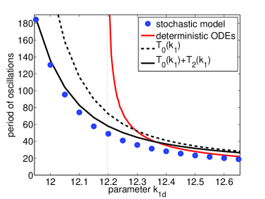
      (a) ​​​​ (b)

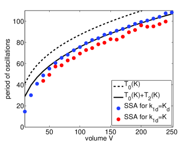
Fig. 13: (a) Approximations of the mean period of oscillation $T_{0}(k_{1})$ and $T_{0}(k_{1})+T_{2}(k_{1})$ given by $(\ref{T0approx})$ and $(\ref{T2approx})$. We also replot the results of Figure 4(a) for comparison. Parameters are the same as in Figure 4(a). (b) Approximations of the mean period of oscillation $T_{0}(K)$ and $T_{0}(K)+T_{2}(K)$ given by $(\ref{T0approx0})$ and $(\ref{T2approx0})$. We also replot the results of Figure 4(b) for comparison. Parameters are given by $(\ref{sniperparam})$.

Transforming (90) into original variables, we can obtained an improved (second-order) approximation of the period of oscillation as $T_{0}(k_{1})+T_{2}(k_{1})$ where

$$T_{2}(k_{1})=\left(\sigma_{17}-\frac{\sigma_{4}\,\sigma_{10}}{\lambda_{0}}-\frac{2\sigma_{18}\,\sigma_{1}}{\lambda_{0}}\right)\frac{\sqrt{3\pi}}{\sigma_{5}\sigma_{8}}\,\,G\!\left(-\left(\frac{12}{\sigma_{5}\,\sigma_{8}^{2}}\right)^{1/3}\sigma_{6}\,(k_{1}-K)\right)$$ (92)

and the constants $\sigma_{i}$, $i=1,4,5,6,8,10,17,18$, are given in Appendix C. Again, the overbars have to be dropped. The approximation $T_{0}(k_{1})+T_{2}(k_{1})$ is plotted in Figure 13(a) as the black solid line.

In Figure 4(b), we studied the period of oscillation as a function of the volume $V$ for $k_{1d}=K_{d}$. To approximate this dependence, we put $k_{1d}=K$ into formulae (91) and (92). Since $G(0)=\sqrt{\pi}/3$ and $H(0)=\Gamma(1/6)/3$, we obtain

$$T_{0}(K) = \sqrt{\pi}\;3^{-5/6}\left(\frac{2}{\sigma_{5}^{2}\,\sigma_{8}}\right)^{1/3}\Gamma(1/6),$$ (93)

$$T_{2}(K) = \left(\sigma_{17}-\frac{\sigma_{4}\,\sigma_{10}}{\lambda_{0}}-\frac{2\sigma_{18}\,\sigma_{1}}{\lambda_{0}}\right)\frac{\pi}{\sigma_{5}\sigma_{8}\sqrt{3}},$$ (94)

where $\Gamma$ is the Gamma function. The values of $T_{0}(K)$ and $T_{0}(K)+T_{2}(K)$ are plotted as functions of the volume $V$ in Figure 13(b). We see that $T_{0}(K)+T_{2}(K)$ compare well with the results obtained by the stochastic simulation for $k_{1d}=K_{d}$. To be more precise, we should compare it with stochastic results obtained for $k_{1d}=K$ where $K$ depends on the volume as shown in Figure 12(a). Such data are plotted in Figure 13(b) too.

Another way to approximate the period of oscillation is to approximate $\overline{d}_{x}(\overline{x},\overline{y},k_{1})$ (resp. $\overline{d}_{xy}(\overline{x},\overline{y},k_{1})$ and $\overline{d}_{y}(\overline{x},\overline{y},k_{1})$) by $\overline{d}_{x}(\overline{q})$ (resp. $\overline{d}_{xy}(\overline{q})$ and $\overline{d}_{y}(\overline{q})$) only in the equation (68). If the approximation of $\overline{v}_{x}(\overline{x},\overline{y},k_{1})$ and $\overline{v}_{y}(\overline{x},\overline{y},k_{1})$ is the same as before, the resulting formulae are equal to (91)–(94) with $\sigma_{17}=0$. The comparison of the results for $\sigma_{17}=0$ is shown in Figure 14. We see that we have an excellent comparison with the results of the stochastic simulation for $k_{1d}=K$ as a function of the volume $V$ - panel Figure 14(b).

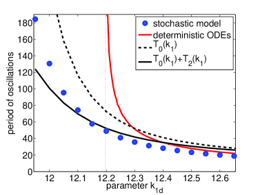
      (a) ​​​​ (b)

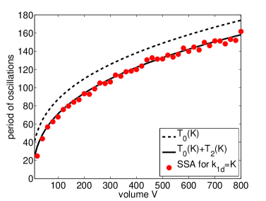
Fig. 14: (a) Approximations of the mean period of oscillation $T_{0}(k_{1})$ and $T_{0}(k_{1})+T_{2}(k_{1})$ given by $(\ref{T0approx})$ and $(\ref{T2approx})$ with $\sigma_{17}=0$. We also replot the results of Figure 4(a) for comparison. Parameters are the same as in Figure 4(a). (b) Approximations of the mean period of oscillation $T_{0}(K)$ and $T_{0}(K)+T_{2}(K)$ given by $(\ref{T0approx0})$ and $(\ref{T2approx0})$ with $\sigma_{17}=0$. We also plot the results obtained by the stochastic simulation for $k_{1d}=K$. The other parameters are given by $(\ref{sniperparam})$.

6 Conclusion

Bifurcation diagrams of ODEs computed by standard numerical continuation methods constitute a systematic way to study and summarize the dependence of the behaviour of the ODE system on its parameters. An exploration of such a dependence could be in principle done by a direct integration in time, but it would be much more computationally intensive than the numerical continuation. In a similar way, the exploration of the dependence of the behaviour of a stochastic chemical model on its parameters can in principle be done by the Gillespie SSA; yet, it is more efficient to study it by solving the underlying stationary Fokker-Planck equation numerically or by analysing it. For example, computation of the mean period of oscillation by the Gillespie SSA is more computationally intensive for large values of the system size (volume $V$) because the large values of $V$ correspond to chemical systems with many molecules. On the other hand, the computational intensity of the FEM solution of the Fokker-Planck equation is independent of $V,$ making it more suitable for studying the dependence of the mean period of oscillation on the volume $V$. The asymptotic formulae (91) and (92) provide further insights into the behaviour of the mean period of oscillation. At the bifurcation point $k_{1d}=K$ of (67), the formula (91) simplifies to (93). Inspecting (93), we conclude that the mean period of oscillation asymptotes to infinity as $V^{1/3}$ for $V\to\infty.$ If $V$ is finite, the stochastic model of the chemical system (1)–(2) possesses oscillatory solutions for any value of $k_{1d}$ which is close to $K$ or close to $K_{d}$ where $k_{1d}=K_{d}$ is the bifurcation point of the classical deterministic ODE model (3)–(4). On the other hand, the trajectories of (3)–(4) only oscillate for $k_{1d}>K_{d}$. The period of oscillation asymptotes to infinity as $(k_{1d}-K_{d})^{-1/2}$ for $k_{1d}\to K_{d}^{+}.$

In this paper, we used an illustrative example of the chemical system with two chemical species for which the deterministic mean-field description is undergoing a SNIPER bifurcation. The system was simple enough that we could directly compute many realisations of the Gillespie SSA. Averaging over many realisations, we estimated important characteristics of the system, for example, the mean period of oscillation. These estimates were used for the visual comparison with the results obtained by the asymptotic analysis of the chemical Fokker-Planck equation and by solving this equation numerically. Another advantage of the illustrative chemical system was that the chemical Fokker-Planck equation was two-dimensional, which simplified its asymptotic analysis and numerical solution. If we have a system of $N$ chemical species, the resulting chemical Fokker-Planck equation will be $N$-dimensional. We are currently investigating the advantages and disadvantages of this approach for $N$ larger than 2. Clearly, a suitable numerical method for solving the higher-dimensional PDEs must be applied. The analysis presented here can also be generalized to higher-dimensional cases. All we need to find are the eigenvectors of the Jacobian matrix at the saddle. The biggest contribution to the mean exit time or the mean period of oscillation will be in the direction of the eigenvector corresponding to the saddle-node connection. Thus the approach presented is potentially equally applicable to the $N$-dimensional case and lead to the estimates of the dependence of the important system characteristics (e.g. the mean period of oscillation) on the model parameters. Alternative methods to obtain these estimates include: accelerating the Gillespie SSA by using approximate SSAs [8], or estimating the low-dimensional effective Fokker-Planck equation by using short bursts of appropriately initialized stochastic simulations [4]. Both approaches use SSAs. In contrast, the methods presented in this paper were based on the numerical solution and asymptotic analysis of PDEs, i.e. no stochastic simulation and no generators of random numbers were needed.

Appendix A Chemical Fokker-Planck equation for $N$-dimensional systems

Let us consider a well-stirred mixture of $N\geq 1$ molecular species that chemically interact through $M\geq 1$ chemical reactions $R_{j}$, $j=1,\dots,M$. The state of this system is described by ${\mathbf{X}}=[X_{1},\dots,X_{N}]$ where $X_{i}\equiv X_{i}(t)$ is the number of molecules of the $i$-th chemical species, $i=1,\dots,N.$ Let $\alpha_{j}({\mathbf{x}})$ be the propensity function of the chemical reaction $R_{j}$, $j=1,\dots,M$, i.e. $\alpha_{j}({\mathbf{x}})\mbox{d}t$ is the probability that, given ${\mathbf{X}}(t)={\mathbf{x}}$, one $R_{j}$ reaction will occur in the next infinitesimal time interval $[t,t+\mbox{d}t)$. Let $\nu_{ji}$ be the change in the number of $X_{i}$ produced by one $R_{j}$ reaction. Then the chemical system can be described by the chemical master equation

$$\frac{\partial}{\partial t}p({\mathbf{x}},t)=\sum_{j=1}^{M}\Big{[}\alpha_{j}({\mathbf{x}}-{\boldsymbol{\nu}}_{j})p({\mathbf{x}}-{\boldsymbol{\nu}}_{j},t)-\alpha_{j}({\mathbf{x}})p({\mathbf{x}},t)\Big{]},$$

where $p({\mathbf{x}},t)$ is the probability that ${\mathbf{X}}(t)={\mathbf{x}}$ and ${\boldsymbol{\nu}}_{j}=[\nu_{j1},\dots,\nu_{jN}]$. Considering the integer valued vector ${\mathbf{x}}$ as a real variable, Gillespie [7] derived the chemical Langevin equation by approximating Poisson random variables by normal random variables. This approximation is possible if many reaction events happen before the propensity functions change significantly their values, see [7] for details. The chemical Langevin equation can be written in the form

$$\mbox{d}X_{i}=\left(\sum_{j=1}^{M}\nu_{ji}\alpha_{j}({\mathbf{X}}(t))\right)\mbox{d}t+\sum_{j=1}^{M}\nu_{ji}\alpha_{j}^{1/2}({\mathbf{X}}(t))\mbox{d}W_{j}$$

which corresponds to the chemical Fokker-Planck equation

$$\frac{\partial}{\partial t}p({\mathbf{x}},t) = \sum_{i=1}^{N}\frac{\partial}{\partial x_{i}}\left[-\left(\sum_{j=1}^{M}\nu_{ji}\alpha_{j}(x)\right)p({\mathbf{x}},t)\right]+\frac{1}{2}\frac{\partial^{2}}{\partial x_{i}^{2}}\left[\left(\sum_{j=1}^{M}\nu^{2}_{ji}\alpha_{j}(x)\right)p({\mathbf{x}},t)\right]$$ (95)

$$+\sum_{k<i}\frac{\partial^{2}}{\partial x_{i}x_{k}}\left[\left(\sum_{j=1}^{M}\nu_{ji}\nu_{jk}\alpha_{j}(x)\right)p({\mathbf{x}},t)\right].$$

Appendix B Equation for the exit time $\tau$

Let $p(x^{\prime},y^{\prime},t;x,y,0)$ be the probability that $X(t)=x^{\prime}$, $Y(t)=y^{\prime}$ given that $X(0)=x$ and $Y(0)=y$. It satisfies the backward Kolmogorov equation

$$\frac{\partial p}{\partial t}=d_{x}\frac{\partial^{2}p}{\partial x^{2}}+d_{xy}\frac{\partial^{2}p}{\partial x\partial y}+d_{y}\frac{\partial^{2}p}{\partial y^{2}}+v_{x}\frac{\partial p}{\partial x}+v_{y}\frac{\partial p}{\partial y}.$$ (96)

Let $h(x,y,t)$ be the probability that $[X(t),Y(t)]\in\Omega$ at time $t$ given that it started at $[X(0),Y(0)]=[x,y].$ Then

$$h(x,y,t)=\int_{\Omega}p(x^{\prime},y^{\prime},t;x,y,0)\,\mbox{d}x^{\prime}\mbox{d}y^{\prime}.$$

Integrating (96), we obtain

$$\frac{\partial h}{\partial t}=d_{x}\frac{\partial^{2}h}{\partial x^{2}}+d_{xy}\frac{\partial^{2}h}{\partial x\partial y}+d_{y}\frac{\partial^{2}h}{\partial y^{2}}+v_{x}\frac{\partial h}{\partial x}+v_{y}\frac{\partial h}{\partial y}.$$ (97)

The mean exit time $\tau$ to leave $\Omega$, given that initially $[X(0),Y(0)]=[x,y]$, can be computed as follows [5]

$$\tau(x,y)=-\int_{0}^{\infty}t\,\frac{\partial h}{\partial t}(x,y,t)\mbox{d}t=\int_{0}^{\infty}h(x,y,t)\mbox{d}t.$$

Integrating equation (97) over $t$, we obtain the following elliptic problem:

$$d_{x}\frac{\partial^{2}\tau}{\partial x^{2}}+d_{xy}\frac{\partial^{2}\tau}{\partial x\partial y}+d_{y}\frac{\partial^{2}\tau}{\partial y^{2}}+v_{x}\frac{\partial\tau}{\partial x}+v_{y}\frac{\partial\tau}{\partial y}=-1,\quad\mbox{for}\;[x,y]\in\Omega.$$ (98)

Appendix C Formulae for coefficients $c_{i}$ and $\omega_{i}$

The coefficients $c_{i}(\overline{d}_{x})$, $c_{i}(\overline{d}_{xy})$, $c_{i}(\overline{d}_{y})$, $c_{i}(\overline{v}_{x})$ and $c_{i}(\overline{v}_{y})$ can be computed by the Taylor expansion. Below, we provide the expressions for those coefficients which actually appear in the final formulae for the mean period of oscillation:

$$c_{1}(\overline{v}_{x})=\displaystyle\frac{\partial^{2}\overline{v}_{x}}{\partial\overline{x}^{2}}(\overline{q})\frac{\overline{u}_{11}^{2}}{2},\qquad c_{2}(\overline{v}_{x})=\displaystyle\frac{\partial^{2}\overline{v}_{x}}{\partial\overline{x}^{2}}(\overline{q})\overline{u}_{11}\overline{u}_{12},\qquad c_{3}(\overline{v}_{x})=\displaystyle\frac{\partial^{2}\overline{v}_{x}}{\partial\overline{x}^{2}}(\overline{q})\frac{\overline{u}_{12}^{2}}{2},$$

$$c_{1}(\overline{v}_{y})=\displaystyle\frac{\partial^{2}\overline{v}_{y}}{\partial\overline{x}^{2}}(\overline{q})\frac{\overline{u}_{11}^{2}}{2}+\displaystyle\frac{\partial^{2}\overline{v}_{y}}{\partial\overline{x}\partial\overline{y}}(\overline{q})\overline{u}_{11}\overline{u}_{21},$$

$$c_{2}(\overline{v}_{y})=\displaystyle\frac{\partial^{2}\overline{v}_{y}}{\partial\overline{x}^{2}}(\overline{q})\overline{u}_{11}\overline{u}_{12}+\displaystyle\frac{\partial^{2}\overline{v}_{y}}{\partial\overline{x}\partial\overline{y}}(\overline{q})(\overline{u}_{11}\overline{u}_{22}+\overline{u}_{12})\overline{u}_{21}),$$

$$c_{3}(\overline{v}_{y})=\displaystyle\frac{\partial^{2}\overline{v}_{y}}{\partial\overline{x}^{2}}(\overline{q})\frac{\overline{u}_{12}^{2}}{2}+\displaystyle\frac{\partial^{2}\overline{v}_{y}}{\partial\overline{x}\partial\overline{y}}(\overline{q})\overline{u}_{12}\overline{u}_{22},\qquad c_{1}(\overline{d}_{x})=\frac{\partial\overline{d}_{x}}{\partial\overline{x}}(\overline{q})\,\overline{u}_{11}+\frac{\partial\overline{d}_{x}}{\partial\overline{y}}(\overline{q})\,\overline{u}_{21},$$

$$c_{1}(\overline{d}_{xy})=\frac{\partial\overline{d}_{xy}}{\partial\overline{x}}(\overline{q})\,\overline{u}_{11}+\frac{\partial\overline{d}_{xy}}{\partial\overline{y}}(\overline{q})\,\overline{u}_{21},\qquad c_{1}(\overline{d}_{y})=\frac{\partial\overline{d}_{y}}{\partial\overline{x}}(\overline{q})\,\overline{u}_{11}+\frac{\partial\overline{d}_{y}}{\partial\overline{y}}(\overline{q})\,\overline{u}_{21},$$

where we used the formulae (52)–(53) to simplify the Taylor expansion of $\overline{v}_{x}(\overline{x},\overline{y},k_{1})$ and $\overline{v}_{y}(\overline{x},\overline{y},k_{1})$. Note that some of the second derivatives of $\overline{v}_{x}$ and $\overline{v}_{y}$ are zero which makes the resulting formulae shorter. However, even if they were nonzero, the same analysis could be carried through. The $\sigma$ coefficients are given by

$$\sigma_{1} = (\det\overline{U})^{-2}\left(\overline{d}_{x}(\overline{q})\overline{u}_{21}^{2}-\overline{d}_{xy}(\overline{q})\overline{u}_{21}\overline{u}_{11}+\overline{d}_{y}(\overline{q})\overline{u}_{11}^{2}\right),$$

$$\sigma_{4} = (\det\overline{U})^{-2}\left(-\overline{d}_{x}(\overline{q})2u_{21}u_{22}+\overline{d}_{xy}(\overline{q})\left(\overline{u}_{11}\overline{u}_{22}+\overline{u}_{12}\overline{u}_{21}\right)-\overline{d}_{y}(\overline{q})2u_{11}u_{12}\right),$$

$$\sigma_{5} = (\det\overline{U})^{-1}\left(c_{1}(\overline{v}_{x})\overline{u}_{22}-c_{1}(\overline{v}_{y})\overline{u}_{12}\right),$$

$$\sigma_{6} = -(\det\overline{U})^{-1}\overline{u}_{12},$$

$$\sigma_{8} = (\det\overline{U})^{-2}\left(\overline{d}_{x}(\overline{q})\overline{u}_{22}^{2}-\overline{d}_{xy}(\overline{q})\overline{u}_{12}\overline{u}_{22}+\overline{d}_{y}(\overline{q})\overline{u}_{12}^{2}\right),$$

$$\sigma_{10} = (\det\overline{U})^{-1}\left(c_{2}(\overline{v}_{x})\overline{u}_{22}-c_{2}(\overline{v}_{y})\overline{u}_{12}\right),$$

$$\sigma_{17} = (\det\overline{U})^{-2}\left(c_{1}(\overline{d}_{x})(\overline{q})\overline{u}_{22}^{2}-c_{1}(\overline{d}_{xy})(\overline{q})\overline{u}_{12}\overline{u}_{22}+c_{1}(\overline{d}_{y})(\overline{q})\overline{u}_{12}^{2}\right),$$

$$\sigma_{18} = (\det\overline{U})^{-1}\left(c_{3}(\overline{v}_{x})\overline{u}_{22}-c_{3}(\overline{v}_{y})\overline{u}_{12}\right).$$

To get the coefficients $\sigma_{i}$ in the final formulae (91)–(94), we simply drop the overbars in the expressions above.

Acknowledgements. This publication is based on work supported by St. John’s College, Oxford; Linacre College, Oxford; Somerville College, Oxford and by Award No. KUK-C1-013-04, made by King Abdullah University of Science and Technology (RE). IGK was supported by the National Science Foundation and the US DOE. TV acknowledges the support of the Czech Science Foundation, project No. 102/07/0496, of the Grant Agency of the Academy of Sciences, project No. IAA100760702, and of the Czech Academy of Sciences, institutional research plan No. AV0Z10190503. The authors also benefited from helpful discussions with Bill Baumann and John Tyson.

References

- [1] R. DeVille, C. Muratov, and E. Vanden-Eijnden, Non-meanfield deterministic limits in chemical reaction kinetics, Journal of Chemical Physics 124 (2006), 231102.
- [2] E. Doedel, H. Keller, and J. Kernévez, Numerical analysis and control of bifurcation problems, part I, Int. J. Bifurcation and Chaos 1 (1991), no. 3, 493–520.
- [3] , Numerical analysis and control of bifurcation problems, part II, Int. J. Bifurcation and Chaos 1 (1991), no. 4, 745–772.
- [4] R. Erban, I. Kevrekidis, D. Adalsteinsson, and T. Elston, Gene regulatory networks: A coarse-grained, equation-free approach to multiscale computation, Journal of Chemical Physics 124 (2006), 084106.
- [5] R. Fox, Functional-calculus approach to stochastic differential equations, Physical Review A 33 (1986), no. 1, 467–476.
- [6] D. Gillespie, Exact stochastic simulation of coupled chemical reactions, Journal of Physical Chemistry 81 (1977), no. 25, 2340–2361.
- [7] , The chemical Langevin equation, Journal of Chemical Physics 113 (2000), no. 1, 297–306.
- [8] , Approximate accelerated stochastic simulation of chemically reacting systems, Journal of Chemical Physics 115 (2001), no. 4, 1716–1733.
- [9] M. Haataja, D. Srolovitz, and I. Kevrekidis, Apparent hysteresis in a driven system with self-organized drag, Physical Review Letters 92 (2004), no. 16, 160603.
- [10] R. Hinch and S. J. Chapman, Exponentially slow transitions on a Markov chain: the frequency of Calcium Sparks, European Journal of Applied Mathematics 16 (2005), 427–446.
- [11] H. Risken, The Fokker-Planck Equation, methods of solution and applications, Springer-Verlag, 1989.
- [12] F. Schlögl, Chemical reaction models for non-equilibrium phase transitions, Zeitschrift für Physik 253 (1972), no. 2, 147–161.
- [13] J. Tyson, A. Csikasz-Nagy, and B. Novak, The dynamics of cell cycle regulation, BioEssays 24 (2002), 1095–1109.
- [14] M. Ward, Exponential asymptotics and convection-diffusion-reaction models, Analyzing Multiscale Phenomena Using Singular Perturbation Methods (J. Cronin and R. O’Malley, eds.), Proceedings of Symposia in Applied Mathematics, vol. 56, AMS, 1999, pp. 151–184.