Issue 1, Volume 1, 2011, 4-18

Fast, exact (but unstable) spin spherical harmonic transforms

Jason D. McEwen
Astrophysics Group, Cavendish Laboratory, University of Cambridge, UK
Institute of Electrical Engineering, Ecole Polytechnique Fédérale de Lausanne (EPFL), Switzerland

Abstract: In many applications data are measured or defined on a spherical manifold; spherical harmonic transforms are then required to access the frequency content of the data. We derive algorithms to perform forward and inverse spin spherical harmonic transforms for functions of arbitrary spin number. These algorithms involve recasting the spin transform on the two-sphere ${\mathrm{S}^{2}}$ as a Fourier transform on the two-torus ${\mathrm{T}^{2}}$. Fast Fourier transforms are then used to compute Fourier coefficients, which are related to spherical harmonic coefficients through a linear transform. By recasting the problem as a Fourier transform on the torus we appeal to the usual Shannon sampling theorem to develop spherical harmonic transforms that are theoretically exact for band-limited functions, thereby providing an alternative sampling theorem on the sphere. The computational complexity of our forward and inverse spin spherical harmonic transforms scale as $\mathcal{O}({L}^{3})$ for any arbitrary spin number, where ${L}$ is the harmonic band-limit of the spin function on the sphere. Numerical experiments are performed and unfortunately the forward transform is found to be unstable for band-limits above ${L}\simeq 32$. The instability is due to the poorly conditioned linear system relating Fourier and spherical harmonic coefficients. The inverse transform is expected to be stable, although it is not possible to verify this hypothesis.

Keywords: spherical harmonics; spherical harmonic transform; two-sphere; algorithms

1 Introduction

Data are defined inherently on the sphere in many practical applications, including computer graphics (e.g. [1]), planetary science (e.g. [2, 3, 4]), solar physics (e.g. [5, 6]), geophysics (e.g. [7, 8, 9]), quantum chemistry (e.g. [10, 11]) and astrophysics (e.g. [12, 13, 14, 15]), for example. In a number of these applications it is insightful to compute the spherical harmonic representation of the data. For example, observations of the anisotropies of the cosmic microwave background (CMB), that are inherently made on the celestial sphere, contain a wealth of information about models of the early Universe. The anisotropies of the CMB are seeded by primordial perturbations, which, in linear perturbation theory, evolve independently for each Fourier mode. Solutions of models of the early Universe are therefore solved more conveniently in Fourier space and manifest themselves in the form of the angular power spectrum of CMB anisotropies. Cosmologists compute the angular power spectrum of observations of the CMB, through a spherical harmonic transform, to make contact with theory and to estimate parameters of cosmological models (e.g. [16]). Recent and upcoming observations of CMB anisotropies made on the celestial sphere are of considerable size, with maps containing approximately three [15] and fifty [17] million pixels respectively.

Consequently, the ability to perform a fast spherical harmonic transform for data of considerable size is essential in assisting cosmologists to understand our Universe.

A number of works have addressed the problem of computing a spherical harmonic transform efficiently. We first survey the related literature for computing the scalar transform on the sphere, before discussing approaches for computing the harmonic transform of spin functions on the sphere. By performing a simple separation of variables the spherical harmonic transform may be rewritten as a Fourier transform and an associated Legendre transform. This already reduces the complexity of computation from $\mathcal{O}({L}^{4})$ to $\mathcal{O}({L}^{3})$, where ${L}$ is the harmonic band-limit defining the maximum frequency content of the function considered (defined mathematically in Sec. 3.1). If this separation of variable is performed first, then to reduce the complexity of the spherical harmonic transform further reduces to the problem of performing a fast associated Legendre transform.

First attempts to compute a scalar spherical harmonic through a fast Legendre transform were performed by Orszag [18] and were based on a Wentzel-Kramers-Brillouin (WKB) approximation. Alternative approaches using the fast multipole method (FMM) [19] have been considered by Alpert & Rokhin [20] and by Suda & Takani [21]. All of these methods are necessarily approximate, for any choice of pixelisation of the sphere, and the complexity of these algorithms scales linearly with the desired accuracy.

Other approaches based on the separation of variables have been developed for particular pixelisations of the sphere, such as HEALPix [22], IGLOO [23] and GLESP [24]. In all of these cases the resulting algorithms are of complexity $\mathcal{O}({L}^{3})$ and for HEALPix and IGLOO pixelisations only approximate quadrature rules exist. Due to the approximate quadrature the spherical harmonic transform algorithms of HEALPix and IGLOO are not theoretically exact; a forward transform followed by an inverse transform will not recover the original signal perfectly, even with exact-precision arithmetic. By contrast GLESP does exhibit an exact quadrature rule due to its adoption of Gauss-Legendre quadrature. All of these pixelisation schemes and their associated harmonic transform algorithms are of sufficient accuracy for many practical purposes and have been of considerable use in the analysis of CMB data.

A sampling theorem on the sphere was first developed by Driscoll & Healy [25], providing a framework for a spherical harmonic transform that is theoretically exact. Moreover, Driscoll & Healy also present a divide-and-conquer approach to computing a fast associated Legendre transform in the cosine basis, using a fast Fourier transform (FFT) to project onto this basis. The resulting algorithm is exact in exact-precision arithmetic and has computational complexity $\mathcal{O}({L}^{2}\log{}_{2}^{2}{L})$, but is known to suffer from stability problems [26, 27]. Potts [28] adapted the Driscoll & Healy approach to use a fast cosine transform (as suggested previously [25]) to reduce computation time, but not complexity, and introduced some stabilisation methods. Healy et al. [26] readdressed the work of Driscoll & Healy, reformulating the sampling theorem on the sphere and developing some variants of the original Driscoll & Healy algorithm. A fast cosine transform is used here and a number of alternative algorithms are presented, including the so-called semi-naive, simple split and hybrid algorithms: the semi-naive algorithm is a more stable variant of the original (non-divide-and-conquer) Driscoll & Healy algorithm with complexity $\mathcal{O}({L}^{3})$; the simple-split algorithm is a simpler and more stable divide-and-conquer approach than the original unstable divide-and-conquer Driscoll & Healy algorithm but with a complexity of $\mathcal{O}({L}^{5/2}\log{}_{2}^{1/2}{L})$; the hybrid algorithm uses both of these two algorithms and splits the problem between them. The hybrid algorithm appears to achieve a good compromise between stability and efficiency. However, the overall complexity of this algorithm is not clear since it depends on the split between the semi-naive and simple split algorithms and on some user specified parameters. Implementations of these algorithms [26] are available for download. Due to the divide-and-conquer approach first proposed by Driscoll & Healy for the fast associated Legendre transform, these algorithms [25, 28, 26] are all restricted to harmonic band-limits that are a power of two.

An alternative algorithm is developed by Mohlenkamp [29, 30], that is again based on a separation of variables and a fast associated Legendre transform. This method is based on the exact sampling theorem on the sphere of Driscoll & Healy and a compressed representation of the associated Legendre functions using WKB frequency estimates. Rigorous bounds are derived for the number of coefficients required to achieve a given accuracy. The method is again necessarily approximate, but the approximation can be controlled independently of complexity. The complexity of this algorithm is $\mathcal{O}({L}^{2}\log{}_{2}^{2}{L})$ and in practice very good accuracy and stability is achieved. However, the algorithm is also restricted to band-limits that are a power of two.

Very little attention has been paid to fast algorithms to perform the spherical harmonic transform of spin functions. Spin functions on the sphere also arise in many applications. For example, the linear polarisation of the CMB anisotropies is described by the Stokes parameters $Q$ and $U$, where the quantity $Q\pm{i}U$ is a spin $\pm 2$ function on the sphere [31]. The reason little attention has been paid explicitly to the transform of spin functions may be because spin lowering and raising operators can be used to relate spin spherical harmonic transforms to the scalar transform. This is done explicitly and in a stable manner by Wiaux et al. [32] for the spin $\pm 2$ case. Scalar spherical harmonic algorithms developed by Healy et al. [26] are then applied to yield a theoretically exact spin $\pm 2$ algorithm with the same complexity as the Healy et al. algorithm that is adopted. In general, this type of approach may be used to compute the spin transform for arbitrary spin, however the complexity of the resulting spin algorithm will be scaled by the spin number.

In this work we derive a general algorithm to perform a spin spherical harmonic transform for functions of arbitrary spin number. The complexity of the algorithm is independent of spin number. Furthermore, any harmonic band-limit may be considered and not only powers of two. Our spin spherical harmonic transform algorithm essentially involves recasting the spin transform on the sphere as a Fourier transform on the torus. FFTs are then used to compute Fourier coefficients, which are related to the spherical harmonic coefficients of the function considered through a linear transform. By recasting the problem as a Fourier transform on the torus we appeal to the usual Shannon sampling theorem [33] to develop spherical harmonic transforms that are theoretically exact for band-limited functions, thereby providing an alternative sampling theorem on the sphere. The remainder of this paper is organised as follows. The mathematical background is presented in Sec. 2. In Sec. 3 we derive our spin transform algorithms and discuss a number of subtleties of the algorithms and practical considerations. In Sec. 4 we examine the memory and computation complexity of the algorithms and evaluate their stability with numerical experiments. Concluding remarks are made in Sec. 5.

2 Mathematical background

Before deriving our fast algorithms it is necessary to outline some mathematical preliminaries. Harmonic analysis of scalar functions on the two-sphere ${\mathrm{S}^{2}}$ and on the rotation group ${\mathrm{SO}(3)}$ is reviewed first, before discussing the analysis of spin functions on ${\mathrm{S}^{2}}$. By making all definitions explicit we hope to avoid any confusion over the conventions adopted. The reader familiar with harmonic analysis on ${\mathrm{S}^{2}}$ and ${\mathrm{SO}(3)}$ may choose to skip this section and refer back to it as required. However, in the final part of Sec. 2.2 we present some important symmetry relations of Wigner functions that are required in the derivation of our algorithms.

2.1 Scalar spherical harmonics

The spherical harmonic functions $Y_{\ell m}({\omega})$, with natural $\ell\in\mathbb{N}$ and integer $m\in\mathbb{Z}$ satisfying $|m|\leq\ell$, form an orthogonal basis in the space of $\mathrm{L}^{2}({\mathrm{S}^{2}},\mathrm{\,d}\Omega(\omega))$ scalar functions on the two-sphere ${\mathrm{S}^{2}}$, where $\omega\equiv(\theta,\varphi)\in{\mathrm{S}^{2}}$ are the spherical coordinates with co-latitude $\theta\in[0,\pi]$ and longitude $\varphi\in[0,2\pi)$ and $\mathrm{\,d}\Omega(\omega)=\sin\theta\mathrm{\,d}\theta\mathrm{\,d}\varphi$ is the usual rotation invariant measure on the sphere. The spherical harmonics are defined by

$$Y_{\ell m}({\theta,\varphi})=\sqrt{\frac{2\ell+1}{4\pi}\frac{(\ell-m)!}{(\ell+m)!}}\>P_{\ell}^{m}({\cos\theta})\>{\rm e}^{{i}m\varphi}\>,$$ (1)

where

$$P_{\ell}^{m}({x})=(-1)^{m}\>\frac{1}{2^{\ell}\ell!}\>(1-x^{2})^{m/2}\>\frac{\mathrm{\,d}^{m}}{\mathrm{\,d}x^{m}}\frac{\mathrm{\,d}^{\ell}}{\mathrm{\,d}x^{\ell}}\>(x^{2}-1)^{\ell}$$ (2)

are the associated Legendre functions. We adopt the Condon-Shortley phase convention, with the $(-1)^{m}$ phase factor included in the definition of the associated Legendre functions, to ensure that the conjugate symmetry relation $Y_{\ell m}^{\ast}({\omega})=(-1)^{m}Y_{{\ell},{-m}}({\omega})$ holds, where the superscript ^∗ denotes complex conjugation. The orthogonality and completeness relations for the spherical harmonics defined in this manner read

$$\int_{{\mathrm{S}^{2}}}\mathrm{\,d}\Omega(\omega)\>Y_{\ell m}({\omega})\>Y_{\ell^{\prime}m^{\prime}}^{\ast}({\omega})=\delta_{{\ell}{\ell^{\prime}}}\delta_{{m}{m^{\prime}}}$$ (3)

and

$$\sum_{\ell=0}^{\infty}\sum_{m=-\ell}^{\ell}Y_{\ell m}({\omega})\>Y_{\ell m}^{\ast}({\omega^{\prime}})=\delta(\omega-\omega^{\prime})$$ (4)

respectively, where $\delta_{{i}{j}}$ is the Kronecker delta, $\delta(\omega-\omega^{\prime})=\delta(\varphi-\varphi^{\prime})\>\delta(\cos\theta-\cos\theta^{\prime})$ and $\delta(x)$ is the Dirac delta function. Since the spherical harmonic functions form a complete, orthogonal basis on the sphere, any square integrable function on the sphere $f\in\mathrm{L}^{2}({\mathrm{S}^{2}},\mathrm{\,d}\Omega(\omega))$ may be represented by the spherical harmonic expansion

$$f(\omega)=\sum_{\ell=0}^{\infty}\sum_{m=-\ell}^{\ell}{f}_{{\ell}{m}}\>Y_{\ell m}({\omega})\>,$$ (5)

where the spherical harmonic coefficients are given by the usual projection on to the spherical harmonic basis functions

$${f}_{{\ell}{m}}=\int_{{\mathrm{S}^{2}}}\mathrm{\,d}\Omega(\omega)\>f(\omega)\>Y_{\ell m}^{\ast}({\omega})\>.$$ (6)

The conjugate symmetry relation of the spherical harmonic coefficients of a real function (i.e. $f^{\ast}=f$) is given by ${f}_{{\ell},{-m}}=(-1)^{m}{f}_{{\ell}{m}}^{\ast}$, which follows directly from the conjugate symmetry of the spherical harmonic functions.

2.2 Wigner functions

We describe here representations of the three-dimensional rotation group ${\mathrm{SO}(3)}$. Any rotation $\mathbf{\rho}\in{\mathrm{SO}(3)}$ is uniquely defined by the Euler angles $\mathbf{\rho}=(\alpha,\beta,\gamma)$, where $\alpha\in[0,2\pi)$, $\beta\in[0,\pi]$ and $\gamma\in[0,2\pi)$. We adopt the $zyz$ Euler convention corresponding to the right-handed rotation of a physical body in a fixed coordinate system about the $z$, $y$ and $z$ axes by $\gamma$, $\beta$ and $\alpha$ respectively (since the axes remain fixed, two rotations about the $z$ axis are performed). The Wigner $D$-functions $D_{mn}^{\ell}(\mathbf{\rho})$, with natural $\ell\in\mathbb{N}$ and integer $m,n\in\mathbb{Z}$ satisfying $|m|,|n|\leq\ell$, are the matrix elements of the irreducible unitary representation of the rotation group ${\mathrm{SO}(3)}$. Moreover, the matrix elements $D_{mn}^{\ell}$ also form an orthogonal basis on $\mathrm{L}^{2}({\mathrm{SO}(3)},\mathrm{\,d}\varrho(\mathbf{\rho}))$, where $\mathrm{\,d}\varrho(\mathbf{\rho})=\sin\beta\mathrm{\,d}\alpha\mathrm{\,d}\beta\mathrm{\,d}\gamma$ is the invariant measure on the rotation group. The orthogonality and completeness relations for the Wigner $D$-functions read

$$\int_{\mathrm{SO}(3)}\mathrm{\,d}\varrho(\mathbf{\rho})\>D_{mn}^{\ell}(\mathbf{\rho})\>D_{m^{\prime}n^{\prime}}^{\ell^{\prime}\ast}(\mathbf{\rho})=\frac{8\pi^{2}}{2\ell+1}\>\delta_{{\ell}{\ell^{\prime}}}\delta_{{m}{m^{\prime}}}\delta_{{n}{n^{\prime}}}$$ (7)

and

$$\sum_{\ell=0}^{\infty}\frac{2\ell+1}{8\pi^{2}}\sum_{m=-\ell}^{\ell}\sum_{n=-\ell}^{\ell}D_{mn}^{\ell}(\mathbf{\rho})\>D_{mn}^{\ell\ast}(\mathbf{\rho}^{\prime})=\delta(\mathbf{\rho}-\mathbf{\rho}^{\prime})$$ (8)

respectively, where $\delta(\mathbf{\rho}-\mathbf{\rho}^{\prime})=\delta(\alpha-\alpha^{\prime})\,\delta(\cos\beta-\cos\beta^{\prime})\,\delta(\gamma-\gamma^{\prime})$. Since the Wigner $D$-functions form a complete, orthogonal basis on the rotation group ${\mathrm{SO}(3)}$, any square integrable function on the rotation group $F\in\mathrm{L}^{2}({\mathrm{SO}(3)},\mathrm{\,d}\varrho(\mathbf{\rho}))$ may be represented by the Wigner $D$-function expansion

$$F(\mathbf{\rho})=\sum_{\ell=0}^{\infty}\frac{2\ell+1}{8\pi^{2}}\sum_{m=-\ell}^{\ell}\sum_{n=-\ell}^{\ell}\>F^{\ell}_{mn}\>D_{mn}^{\ell}(\mathbf{\rho})\>,$$ (9)

where the Wigner harmonic coefficients are again given in the usual manner by

$$F^{\ell}_{mn}=\int_{\mathrm{SO}(3)}\mathrm{\,d}\varrho(\mathbf{\rho})\>F(\mathbf{\rho})\>D_{mn}^{\ell\ast}(\mathbf{\rho})\>.$$ (10)

The Wigner $D$-functions may be decomposed in terms of the reduced Wigner $d$-functions by

$$D_{mn}^{\ell}(\alpha,\beta,\gamma)={\rm e}^{-{i}m\alpha}\>d_{mn}^{\ell}(\beta)\>{\rm e}^{-{i}n\gamma}\>.$$ (11)

The real $d$-functions may be defined by

$$d_{mn}^{\ell}(\beta)= \sqrt{\frac{(\ell+n)!(\ell-n)!}{(\ell+m)!(\ell-m)!}}\left(\sin\frac{\beta}{2}\right)^{n-m}$$

$$\times\left(\cos\frac{\beta}{2}\right)^{n+m}P_{\ell-n}^{(n-m,n+m)}({\cos\beta})\>,$$ (12)

where $P_{\ell}^{(a,b)}({\cdot})$ are the Jacobi polynomials. For alternative definitions of the $d$-functions see the selection compiled in [34] and references therein. Recursion formulae and symmetry relations may be used to compute rapidly the Wigner functions in the basis of either complex [35, 27] or real [36, 37] spherical harmonics. In the implementations described in this work, we employ the recursion formulae described in [35].

The $d$-functions satisfy a number of symmetry relations. In this work we make use of the symmetry relations

$$d_{mn}^{\ell}(\beta)=(-1)^{m-n}\>d_{-m,-n}^{\ell}(\beta)\>\>,$$ (13)

$$d_{mn}^{\ell}(\pi-\beta)=(-1)^{\ell-n}\>d_{-m,n}^{\ell}(\beta)$$ (14)

and

$$d_{mn}^{\ell}(-\beta)=(-1)^{m-n}\>d_{mn}^{\ell}(\beta)\>,$$ (15)

which may be found in [38]. In the derivation of our fast spin spherical harmonic transform we often consider $d$-functions of the form $d_{mn}^{\ell}(\pi/2)$. For this special case, we may infer

$$d_{-m,n}^{\ell}(\pi/2)=(-1)^{\ell+m}\>d_{-m,-n}^{\ell}(\pi/2)$$ (16)

from (13) and (14), which implies that $d_{mn}^{\ell}(\pi/2)$ is zero for $n=0$ and odd $\ell+m$. We make continual use of these symmetry relations later in the derivation of our fast algorithms.

Finally, we note an important Wigner $d$-function decomposition. The $d$-function for an arbitrary argument may be decomposed into sums of $d$-functions for a constant argument of $\pi/2$ [39, 35]:

$$d_{mn}^{\ell}(\beta)={i}^{n-m}\sum_{m^{\prime}=-\ell}^{\ell}d_{m^{\prime}m}^{\ell}(\pi/2)\>d_{m^{\prime}n}^{\ell}(\pi/2)\>{\rm e}^{{i}m^{\prime}\beta}\>,$$ (17)

which follows from a factoring of rotations [35]. The Fourier series representation of $d_{mn}^{\ell}(\beta)$ specified by (17) allows one to write the spherical harmonic expansion of a function $f$ on ${\mathrm{S}^{2}}$ in terms of a Fourier series expansion of $f$ on the two-torus ${\mathrm{T}^{2}}$, with $f$ appropriately extended to this domain (as discussed in more detail in section Sec. 3.2). Consequently, (17) is fundamental to the derivation of our fast algorithms.

2.3 Spin spherical harmonics

Spin functions on the sphere ${{}_{s}f}\in\mathrm{L}^{2}({\mathrm{S}^{2}},\mathrm{\,d}\Omega(\omega))$, with integer spin $s\in\mathbb{Z}$, are defined by their behaviour under local rotations. By definition, a spin function transforms as

$${{}_{s}f}^{\prime}(\omega)={\rm e}^{-{i}s\chi}\>{{}_{s}f}(\omega)$$ (18)

under a local rotation by $\chi$, where the prime denotes the rotated function. It is important to note that the rotation considered here is not a global rotation on the sphere, such as that represented by an element of the rotation group ${\mathrm{SO}(3)}$, but rather a rotation by $\chi$ in the tangent plane at $\omega$. The sign convention that we adopt here for the argument of the complex exponential in (18) differs to the original definition [40] but is identical to the convention used recently in the context of the polarisation of the CMB [31].

The spin spherical harmonics ${{}_{s}Y_{\ell m}({\theta,\varphi})}$ form an orthogonal basis for $\mathrm{L}^{2}({\mathrm{S}^{2}},\mathrm{\,d}\Omega(\omega))$ spin $s$ functions on the sphere for $|s|\leq\ell$. Spin spherical harmonics were first developed by Newman & Penrose [40] and were soon realised to be closely related to the Wigner $D$-functions by Goldberg [41]. Spin functions may be defined equivalently from the expansion in Wigner $D$-functions $D_{mn}^{\ell}(\alpha,\beta,\gamma)$ of a function in $\mathrm{L}^{2}({\mathrm{SO}(3)},\mathrm{\,d}\varrho(\mathbf{\rho}))$ evaluated at $\gamma=0$, for fixed $n$. Consequently, the functions $D_{ms}^{\ell}(\varphi,\theta,0)$ or $D_{m,-s}^{\ell\>\ast}(\varphi,\theta,0)$, for fixed $s$, naturally define an orthogonal basis for the expansion of spin $s$ functions on the sphere. The appropriately normalised spin spherical harmonics may therefore be given by

$${{}_{s}Y_{\ell m}({\theta,\varphi})}=(-1)^{s}\sqrt{\frac{2\ell+1}{4\pi}}\>D_{m,-s}^{\ell\>\ast}(\varphi,\theta,0)\>.$$ (19)

Noting the decomposition given by (11), the spin spherical harmonics may also be defined in terms of the reduced Wigner $d$-functions:

$${{}_{s}Y_{\ell m}({\theta,\varphi})}=(-1)^{s}\sqrt{\frac{2\ell+1}{4\pi}}\>d_{m,-s}^{\ell}(\theta)\>{\rm e}^{{i}m\varphi}\>.$$ (20)

For completeness, we also state the explicit expression derived by [41] for the spin spherical harmonics:

$${{}_{s}Y_{\ell m}({\theta,\varphi})}=\sqrt{\frac{2\ell+1}{4\pi}\frac{(\ell+m)!(\ell-m)!}{(\ell+s)!(\ell-s)!}}$$

$$\quad\times\sin^{2\ell}(\theta/2)\>{\rm e}^{{i}m\varphi}$$

$$\quad\times\sum_{r}\Biggl{[}\binom{\ell-s}{r}\binom{\ell+s}{s-m+r}$$

$$\quad\quad\quad\quad\times(-1)^{\ell-s-r}\cot^{s-m+2r}(\theta/2)\Biggr{]}\>,$$ (21)

where the sum is performed over all values of $r$ such that the arguments of the factorials are non-negative. The scalar spherical harmonics are identified with the spin spherical harmonics for spin $s=0$, through the relation

$$d_{m0}^{\ell}(\theta)=\sqrt{\frac{(\ell-m)!}{(\ell+m)!}}\>P_{\ell}^{m}({\cos\theta})\>,$$ (22)

i.e. ${{}_{0}Y_{\ell m}({\omega})}=Y_{\ell m}({\omega})$. The conjugate symmetry relation given for the scalar spherical harmonics generalises to the spin spherical harmonics by ${{}_{s}Y_{\ell m}^{\ast}({\omega})}=(-1)^{s+m}{{}_{-s}Y_{{\ell},{-m}}({\omega})}$.

The orthogonality and completeness of the spin spherical harmonics follows from the orthogonality and completeness of the Wigner $D$-functions and read

$$\int_{{\mathrm{S}^{2}}}\mathrm{\,d}\Omega(\omega)\>{{}_{s}Y_{\ell m}({\omega})}\>{{}_{s}Y_{\ell^{\prime}m^{\prime}}^{\ast}({\omega})}=\delta_{{\ell}{\ell^{\prime}}}\delta_{{m}{m^{\prime}}}$$ (23)

and

$$\sum_{\ell=0}^{\infty}\sum_{m=-\ell}^{\ell}{{}_{s}Y_{\ell m}({\omega})}\>{{}_{s}Y_{\ell m}^{\ast}({\omega^{\prime}})}=\delta(\omega-\omega^{\prime})$$ (24)

respectively. The spin spherical harmonics form a complete, orthogonal basis for spin functions on the sphere, hence any square integral spin $s$ function on the sphere ${}_{s}f\in\mathrm{L}^{2}({\mathrm{S}^{2}},\mathrm{\,d}\Omega(\omega))$ may be represented by the spin $s$ spherical harmonic expansion

$${{}_{s}f}(\omega)=\sum_{\ell=0}^{\infty}\sum_{m=-\ell}^{\ell}{{{}_{s}f}}_{{\ell}{m}}\>{{}_{s}Y_{\ell m}({\omega})}\>,$$ (25)

where the spin spherical harmonic coefficients are given in the usual manner by

$${{{}_{s}f}}_{{\ell}{m}}=\int_{{\mathrm{S}^{2}}}\mathrm{\,d}\Omega(\omega)\,{{}_{s}f}(\omega)\>{{}_{s}Y_{\ell m}^{\ast}({\omega})}\>.$$ (26)

The conjugate symmetry relation of the spin spherical harmonic coefficients is given by ${}_{-s}{f}_{{\ell},{-m}}=(-1)^{s+m}\>{{{}_{s}f}}_{{\ell}{m}}^{\ast}$ for a function satisfying ${{}_{s}f}^{\ast}={{}_{-s}f}$ (which, for a spin $s=0$ function, reduces to the usual reality condition $f^{\ast}=f$ for scalar functions) and follows directly from the conjugate symmetry of the spin spherical harmonics.

Spin raising and lowering operators, $\eth$ and $\bar{\eth}$ respectively, exist so that spin $s\pm 1$ functions may be defined from spin $s$ functions [40, 41]. When applied to a spin $s$ function the resulting function transforms as $(\eth{{}_{s}f})^{\prime}(\omega)={\rm e}^{-{i}(s+1)\chi}(\eth{{}_{s}f})(\omega)$ and $(\bar{\eth}{{}_{s}f})^{\prime}(\omega)={\rm e}^{-{i}(s-1)\chi}(\bar{\eth}{{}_{s}f})(\omega)$, where the primed function again corresponds to a rotation by $\chi$ in the tangent plane at $\omega$. The spin operators are given explicitly by

$$\eth{{}_{s}f}=-\sin^{s}\theta\biggl{(}\frac{\partial}{\partial\theta}+\frac{{i}}{\sin\theta}\frac{\partial}{\partial\varphi}\biggr{)}\sin^{-s}\theta\>{{}_{s}f}$$ (27)

and

$$\bar{\eth}{{}_{s}f}=-\sin^{-s}\theta\biggl{(}\frac{\partial}{\partial\theta}-\frac{{i}}{\sin\theta}\frac{\partial}{\partial\varphi}\biggr{)}\sin^{s}\theta\>{{}_{s}f}\>.$$ (28)

3 Fast algorithms

The harmonic formulation of our fast spherical harmonic transform algorithm for spin functions on the sphere is derived here and contains the essence of the fast algorithm. The harmonic formulation involves recasting the spherical harmonic transform on the sphere as a Fourier series expansion on the torus. A number of subtleties then arise due to the method used to extend a function defined on the sphere to the torus and associated symmetry properties. After discussing these subtleties we then present the fast forward an inverse spin transforms in detail, including a number of practical issues pertaining to an implementation.

3.1 Harmonic formulation

Although we initially wish to compute the spherical harmonic coefficients ${{{}_{s}f}}_{{\ell}{m}}$ of a spin $s$ function ${{}_{s}f}\in\mathrm{L}^{2}({\mathrm{S}^{2}},\mathrm{\,d}\Omega(\omega))$, i.e. we wish to evaluate the forward transform specified by (26), we will instead consider the inverse transform specified by (25). Using the inverse transform to relate the function ${{}_{s}f}$ to its spherical harmonic coefficients ${{{}_{s}f}}_{{\ell}{m}}$ has the advantage that it doesn’t require any quadrature rule to approximate an integral over the sphere and, consequently, it is exact, up to numerical precision. It will then be possible to construct a fast and exact direct transform by inverting the harmonic representation of the fast inverse transform.

Starting with the representation of the spin spherical harmonics in terms of the reduced Wigner $d$-functions given by (20), and then substituting the $d$-function decomposition given by (17), the spin spherical harmonics can be written in terms of a sum of weighted complex exponentials:

$${{}_{s}Y_{\ell m}({\theta,\varphi})}=(-1)^{s}\>{i}^{-(m+s)}\>\sqrt{\frac{2\ell+1}{4\pi}}\>$$

$$\quad\times\sum_{m^{\prime}=-\ell}^{\ell}d_{m^{\prime}m}^{\ell}(\pi/2)\>d_{m^{\prime},-s}^{\ell}(\pi/2)\>{\rm e}^{{i}(m\varphi+m^{\prime}\theta)}\>.$$ (29)

Substituting this expression for the spin spherical harmonics into the inverse spin spherical harmonic transform defined by (25), we obtain

$${{}_{s}f}(\theta,\varphi)=\sum_{\ell=0}^{L}\sum_{m=-\ell}^{\ell}{{{}_{s}f}}_{{\ell}{m}}\>(-1)^{s}\>{i}^{-(m+s)}\>\sqrt{\frac{2\ell+1}{4\pi}}\>$$

$$\times\sum_{m^{\prime}=-\ell}^{\ell}d_{m^{\prime}m}^{\ell}(\pi/2)\>d_{m^{\prime},-s}^{\ell}(\pi/2)\>{\rm e}^{{i}(m\varphi+m^{\prime}\theta)}\>,$$ (30)

where we assume that ${{}_{s}f}$ is band-limited at ${L}$, that is ${{{}_{s}f}}_{{\ell}{m}}=0$, $\forall\ell>{L}$, so that the outer summation may be truncated to ${L}$. After interchanging the orders of summation, (3.1) may be written as

$${{}_{s}f}(\theta,\varphi)=\sum_{m=-{L}}^{L}\sum_{m^{\prime}=-{L}}^{L}{}_{s}F_{mm^{\prime}}\>{\rm e}^{{i}(m\varphi+m^{\prime}\theta)}\>,$$ (31)

where

$${}_{s}F_{mm^{\prime}}=(-1)^{s}\>{i}^{-(m+s)}$$

$$\quad\times\sum_{\ell=0}^{L}\sqrt{\frac{2\ell+1}{4\pi}}\>d_{m^{\prime}m}^{\ell}(\pi/2)\>d_{m^{\prime},-s}^{\ell}(\pi/2)\>{{{}_{s}f}}_{{\ell}{m}}\>.$$ (32)

We adopt the convention that all terms indexed by $\ell$ and an azimuthal index such as $m$ are zero for $|m|>\ell$. This convention may also be represented explicitly by replacing the lower limit of the $\ell$ summation of $0$ in (3.1) with $\max(|m|,|m^{\prime}|)$.

Notice that (31) is very similar to the Fourier series representation of ${{}_{s}f}$. However, the Fourier series expansion is only defined for functions that are periodic, i.e. for functions defined on the torus. A function ${{}_{s}f}$ on the sphere is periodic in $\varphi$ but not in $\theta$. In order to apply (31) directly it is necessary to extend ${{}_{s}f}$, initially defined on the two-sphere ${\mathrm{S}^{2}}$, to be defined on the two-torus ${\mathrm{T}^{2}}$. Once ${{}_{s}f}$ is extended in this manner an inverse FFT may be used to evaluate ${}_{s}F_{mm^{\prime}}$ rapidly from a sampled version of ${{}_{s}f}$. The harmonic coefficients ${{{}_{s}f}}_{{\ell}{m}}$ may then be computed from ${}_{s}F_{mm^{\prime}}$ by inverting (3.1) to give a fast forward spin spherical harmonic transform. Similarly, ${{}_{s}f}$ may be reconstructed by computing ${}_{s}F_{mm^{\prime}}$ from the harmonic coefficients ${{{}_{s}f}}_{{\ell}{m}}$ through (3.1), followed by the use of a forward FFT to recover a sampled version of ${{}_{s}f}$ from ${}_{s}F_{mm^{\prime}}$. This gives a fast inverse spin spherical harmonic transform. By recasting the spherical harmonic expansion on the sphere as a Fourier expansion on the torus we may appeal to the exact quadrature of the Fourier integral on uniformly sampled grids, i.e. the Shannon sampling theorem [33]. Consequently, our fast transforms are theoretically exact (to numerical precision and stability) for a sampling of the sphere compatible with a uniform grid on the torus (a corresponding sampling of the sphere is made explicit in Sec. 3.4.1). We address the periodic extension of ${{}_{s}f}$ from ${\mathrm{S}^{2}}$ to ${\mathrm{T}^{2}}$ next.

3.2 Extending the sphere to the torus

When periodically extending ${{}_{s}f}$ from ${\mathrm{S}^{2}}$ to ${\mathrm{T}^{2}}$ it is important to ensure that all relations used previously are still satisfied on the new domain. Careful attention must therefore be paid to the periodic extension of ${{}_{s}f}$, as a naive extension may introduce inconsistency.

We extend ${{}_{s}f}$ to ${}_{s}\tilde{f}\in\mathrm{L}^{2}({\mathrm{T}^{2}},\mathrm{\,d}^{2}\mbox{\boldmath${x}$})$ by allowing $\theta$ to range over the domain $[-\pi,\pi)$ and assuming ${}_{s}\tilde{f}$ is periodic with period $2\pi$ in both $\varphi$ and $\theta$ (note that $\mathrm{\,d}^{2}\mbox{\boldmath${x}$}=\mathrm{\,d}\theta\mathrm{\,d}\varphi$ is the invariant measure on the $(\theta,\varphi)$-plane). Equivalently, we may represent $\theta\in[0,2\pi)$ and both domains are used interchangeably depending on which is most convenient. Representing ${{}_{s}f}$ over this extended domain is redundant, covering the sphere exactly twice. Nevertheless, such a representation facilitates our fast algorithm, which more than compensates for this redundancy. Such an approach is not uncommon, as [25, 26] also oversample a function on the sphere in the $\theta$ direction in order to develop alternative fast scalar spherical harmonic transforms.

The method used to extend ${{}_{s}f}$ to the new $2\pi$ $\theta$ domain remains to be chosen. Two natural candidates are to extend ${{}_{s}f}$ in $\theta$ in either an even or odd manner about zero. We obtain two candidate periodic extensions of ${{}_{s}f}$ on ${\mathrm{T}^{2}}$: ${}_{s}\tilde{f}^{\rm e}$ and ${}_{s}\tilde{f}^{\rm o}$, where the superscripts denote the even and odd extensions respectively, i.e. ${}_{s}\tilde{f}^{\rm e}(-\theta,\varphi)={}_{s}\tilde{f}^{\rm e}(\theta,\varphi)$ and ${}_{s}\tilde{f}^{\rm o}(-\theta,\varphi)=-{}_{s}\tilde{f}^{\rm o}(\theta,\varphi)$. The appropriate periodic extension to use depends on the symmetry properties of the basis functions used to represent the inverse spherical harmonic transform. In Fig. 1 we illustrate these periodic extensions of a function on the sphere to give a function defined on the torus. We use an Earth topography map to define our initial function on the sphere in this example.

Let us recall the inverse spin spherical harmonic transform given by (25). To ensure consistency, we should extend ${{}_{s}f}$ to ${\mathrm{T}^{2}}$ so that it satisfies the same symmetry properties as ${{}_{s}Y_{\ell m}}$ would when extended to this domain. For the spin $s=0$ case, one might naively expect that $Y_{\ell m}$ would exhibit even symmetry in $\theta$ about zero when extended to $\theta\in[-\pi,\pi)$ based on the definition of $Y_{\ell m}$ given by (1). However, in deriving the alternative harmonic formulation of the inverse spherical harmonic transform in Sec. 3.1 we used the representation of ${{}_{s}Y_{\ell m}}$ specified by (20), or equivalently (2.3). Although all of these definitions are obviously identical on the sphere ${\mathrm{S}^{2}}$, they are not necessarily identical on the torus ${\mathrm{T}^{2}}$. Since we have used (20) in our harmonic formulation we must be sure to satisfy the symmetry properties of this relation on ${\mathrm{T}^{2}}$. The symmetry of (20) in $\theta$ is identical to the symmetry of $d_{ms}^{\ell}(\theta)$. Recall from (15) that

$$d_{ms}^{\ell}(-\theta)=(-1)^{m+s}\>d_{ms}^{\ell}(\theta)\>,$$ (33)

i.e. $d_{ms}^{\ell}(\theta)$ is even for even $m+s$ and odd for odd $m+s$. This same symmetry property is also apparent from (2.3). This symmetry could naively appear to be problematic. There is no way we can extend ${{}_{s}f}$ to ${\mathrm{T}^{2}}$ to satisfy this relation. However, we may solve this problem by considering both $\tilde{f}^{\rm e}$ and $\tilde{f}^{\rm o}$. For even $m+s$, (33) will be satisfied for ${}_{s}\tilde{f}^{\rm e}$, whereas for odd $m+s$ it will be satisfied for ${}_{s}\tilde{f}^{\rm o}$.

Our fast spherical harmonic transform then proceeds as follows. We perform two inverse FFTs to compute rapidly ${}_{s}\tilde{F}_{mm^{\prime}}^{\rm e}$ and ${}_{s}\tilde{F}_{mm^{\prime}}^{\rm o}$ for both ${}_{s}\tilde{f}^{\rm e}$ and ${}_{s}\tilde{f}^{\rm o}$ respectively. We then invert (3.1) to compute the harmonic coefficients ${{}_{s}\tilde{f}}_{{\ell}{m}}^{\rm e}$ and ${{}_{s}\tilde{f}}_{{\ell}{m}}^{\rm o}$ corresponding to ${}_{s}\tilde{f}^{\rm e}$ and ${}_{s}\tilde{f}^{\rm o}$ respectively. The harmonic coefficients ${{{}_{s}f}}_{{\ell}{m}}$ of ${{}_{s}f}$ will be identical to ${{}_{s}\tilde{f}}_{{\ell}{m}}^{\rm e}$ for $m+s$ even only, and the identical to ${{}_{s}\tilde{f}}_{{\ell}{m}}^{\rm o}$ for $m+s$ odd only, i.e.

$${{{}_{s}f}}_{{\ell}{m}}=\begin{cases}{{}_{s}\tilde{f}}_{{\ell}{m}}^{\rm e}&m+s\mbox{ even}\\ {{}_{s}\tilde{f}}_{{\ell}{m}}^{\rm o}&m+s\mbox{ odd}\\ \end{cases}\>.$$ (34)

         

(a) ${{}_{s}f}\in\mathrm{L}^{2}({\mathrm{S}^{2}},\mathrm{\,d}\Omega(\omega))$

(b) ${}_{s}\tilde{f}^{\rm e}\in\mathrm{L}^{2}({\mathrm{T}^{2}},\mathrm{\,d}^{2}\mbox{\boldmath${x}$})$

(c) ${}_{s}\tilde{f}^{\rm o}\in\mathrm{L}^{2}({\mathrm{T}^{2}},\mathrm{\,d}^{2}\mbox{\boldmath${x}$})$

Figure 1: Periodic extension to the torus of Earth topography data defined originally on the sphere (mountains are shown in white and lakes in dark red/grey, with the colour of intermediate values interpolated between these extremes). The left panel shows the Earth data defined on the sphere, while the centre panel shows the even periodic extension of the data to the torus and the right panel shows the odd periodic extension. Both types of periodic extension are used in our fast algorithm.

3.3 Symmetry relations

The Fourier coefficients ${}_{s}F_{mm^{\prime}}$ satisfy a number of symmetry relations which may be exploited to increase the speed of implementations. Here we examine the symmetry properties of ${}_{s}F_{mm^{\prime}}$ using two separate approaches. Firstly, we determine the symmetries of ${}_{s}\tilde{F}_{mm^{\prime}}^{\rm e}$ and ${}_{s}\tilde{F}_{mm^{\prime}}^{\rm o}$ based on the Fourier series representations of ${}_{s}\tilde{f}^{\rm e}$ and ${}_{s}\tilde{f}^{\rm o}$. Secondly, we examine the symmetries of ${}_{s}F_{mm^{\prime}}$ computed directly from ${{{}_{s}f}}_{{\ell}{m}}$ using (3.1). Recall that the symmetries of ${}_{s}F_{mm^{\prime}}$ will only be satisfied by ${}_{s}\tilde{F}_{mm^{\prime}}^{\rm e}$ for $m+s$ even and by ${}_{s}\tilde{F}_{mm^{\prime}}^{\rm o}$ for $m+s$ odd.

Although in practice we will compute ${}_{s}\tilde{F}_{mm^{\prime}}^{\rm e}$ and ${}_{s}\tilde{F}_{mm^{\prime}}^{\rm o}$ by taking FFTs of sampled versions of ${}_{s}\tilde{f}^{\rm e}$ and ${}_{s}\tilde{f}^{\rm o}$ respectively, we may nevertheless represent ${}_{s}\tilde{F}_{mm^{\prime}}^{\rm e}$ and ${}_{s}\tilde{F}_{mm^{\prime}}^{\rm o}$ by the usual projection of the continuous functions on to the complex exponentials, i.e.

$${}_{s}\tilde{F}_{mm^{\prime}}=\frac{1}{(2\pi)^{2}}\int_{0}^{2\pi}\mathrm{\,d}\theta\int_{0}^{2\pi}\mathrm{\,d}\varphi\>{}_{s}\tilde{f}(\theta,\varphi)\>{\rm e}^{-{i}(m\varphi+m^{\prime}\theta)}\>,$$ (35)

where, here and subsequently, we drop the superscript denoting the even or odd function to indicate that the relation holds for both (in fact, the discrete Fourier transform merely gives an exact quadrature rule for evaluating (35)). By considering all combinations of negative $m$ and $m^{\prime}$ we obtain trivially the following symmetry relations for ${}_{s}\tilde{F}_{mm^{\prime}}^{\rm e}$from (35):

$${}_{s}\tilde{F}_{m,-m^{\prime}}^{\rm e} ={}_{s}\tilde{F}_{mm^{\prime}}^{\rm e};$$ (36)

$${}_{-s}\tilde{F}_{-m,m^{\prime}}^{\rm e} ={}_{s}\tilde{F}_{mm^{\prime}}^{\rm e}{}^{\ast}\quad\mbox{for ${{}_{s}f}^{\ast}={{}_{-s}f}$};$$ (37)

$${}_{-s}\tilde{F}_{-m,-m^{\prime}}^{\rm e} ={}_{s}\tilde{F}_{mm^{\prime}}^{\rm e}{}^{\ast}\quad\mbox{for ${{}_{s}f}^{\ast}={{}_{-s}f}$}.$$ (38)

Similarly, we obtain the following symmetry relations for ${}_{s}\tilde{F}_{mm^{\prime}}^{\rm o}$:

$${}_{s}\tilde{F}_{m,-m^{\prime}}^{\rm o} =(-1)\>{}_{s}\tilde{F}_{mm^{\prime}}^{\rm o};$$ (39)

$${}_{-s}\tilde{F}_{-m,m^{\prime}}^{\rm o} =(-1)\>{}_{s}\tilde{F}_{mm^{\prime}}^{\rm o}{}^{\ast}\quad\mbox{for ${{}_{s}f}^{\ast}={{}_{-s}f}$};$$ (40)

$${}_{-s}\tilde{F}_{-m,-m^{\prime}}^{\rm o} ={}_{s}\tilde{F}_{mm^{\prime}}^{\rm o}{}^{\ast}\quad\mbox{for ${{}_{s}f}^{\ast}={{}_{-s}f}$}.$$ (41)

Now we derive symmetry relations for ${}_{s}F_{mm^{\prime}}$ computed directly from ${{{}_{s}f}}_{{\ell}{m}}$ through (3.1). Firstly, we find

$${}_{s}F_{m,-m^{\prime}} =(-1)^{s}\>{i}^{-(m+s)}$$

$$\quad\times\sum_{\ell=0}^{L}\Biggl{[}\sqrt{\frac{2\ell+1}{4\pi}}\>d_{-m^{\prime},m}^{\ell}(\pi/2)\>$$

$$\quad\quad\quad\quad\times d_{-m^{\prime},-s}^{\ell}(\pi/2)\>{{{}_{s}f}}_{{\ell}{m}}\Biggr{]}$$

$$=(-1)^{s}\>{i}^{-(m+s)}$$

$$\quad\times\sum_{\ell=0}^{L}\Biggl{[}\sqrt{\frac{2\ell+1}{4\pi}}\>(-1)^{\ell+m}\>d_{m^{\prime}m}^{\ell}(\pi/2)\>$$

$$\quad\quad\quad\quad\times(-1)^{\ell-s}\>d_{m^{\prime},-s}^{\ell}(\pi/2)\>{{{}_{s}f}}_{{\ell}{m}}\Biggr{]}$$

$$=(-1)^{m+s}\>{}_{s}F_{mm^{\prime}}\>,$$ (42)

where in the second line we have applied the $d$-function symmetry relation (14). For the second symmetry relation we find

$${}_{-s}F_{-m,m^{\prime}} =(-1)^{s}\>{i}^{m+s}$$

$$\quad\times\sum_{\ell=0}^{L}\Biggl{[}\sqrt{\frac{2\ell+1}{4\pi}}\>d_{m^{\prime},-m}^{\ell}(\pi/2)\>$$

$$\quad\quad\quad\quad\times d_{m^{\prime}s}^{\ell}(\pi/2)\>{}_{-s}{f}_{{\ell},{-m}}\Biggr{]}$$

$$=(-1)^{s}\>({i}^{\ast})^{-(m+s)}$$

$$\quad\times\sum_{\ell=0}^{L}\Biggl{[}\sqrt{\frac{2\ell+1}{4\pi}}\>d_{m^{\prime}m}^{\ell}(\pi/2)\>$$

$$\quad\quad\quad\quad\times d_{m^{\prime},-s}^{\ell}(\pi/2)\>(-1)^{m+s}{}_{s}{f}_{{\ell}{m}}^{\ast}\Biggr{]}$$

$$=(-1)^{m+s}\>{}_{s}F_{mm^{\prime}}{}^{\ast}\quad\mbox{for ${{}_{s}f}^{\ast}={{}_{-s}f}$},$$ (43)

where in the second line we have applied the $d$-function symmetry relations (13) and (14), and noted the harmonic conjugate symmetry relation for ${{}_{s}f}^{\ast}={{}_{-s}f}$. It is possible to derive the third symmetry relation for ${}_{s}F_{mm^{\prime}}$ in a similar manner to the previous two, however it is much easier to use these two previously derived relations directly, in which case it may be shown trivially that

$${}_{-s}F_{-m,-m^{\prime}}={}_{s}F_{mm^{\prime}}{}^{\ast}\quad\mbox{for ${{}_{s}f}^{\ast}={{}_{-s}f}$}.$$ (44)

Notice that, as expected, we find that the symmetry relations of ${}_{s}F_{mm^{\prime}}$ are only satisfied by ${}_{s}\tilde{F}_{mm^{\prime}}^{\rm e}$ for $m+s$ even and by ${}_{s}\tilde{F}_{mm^{\prime}}^{\rm o}$ for $m+s$ odd.

For a complex signal we have a single symmetry relation, which may be exploited to speed up an implementation by a factor of two. For a signal satisfying ${{}_{s}f}^{\ast}={{}_{-s}f}$ (i.e. a real signal for the case $s=0$), we have two symmetry relations, which may be exploited to speed up an implementation by a factor of four. These enhancements are of practical importance but do not change the overal scaling of our algorithms.

3.4 Forward and inverse transform

The harmonic formulation of our fast algorithm was derived in Sec. 3.1. Since this derivation a number of practicalities have been discussed, such as extending ${{}_{s}f}$ defined on ${\mathrm{S}^{2}}$ to give ${}_{s}\tilde{f}$ defined on ${\mathrm{T}^{2}}$, and the symmetry properties of the Fourier coefficients of ${}_{s}\tilde{f}$ on ${\mathrm{T}^{2}}$. We are now in a position to describe our fast algorithm in detail. Firstly, we consider the discretisation of ${}_{s}\tilde{f}$ on ${\mathrm{T}^{2}}$ and the inversion of (31) using an FFT to compute ${}_{s}\tilde{F}_{mm^{\prime}}$ rapidly. We then consider the inversion of (3.1) to compute the spherical harmonic coefficients ${{{}_{s}f}}_{{\ell}{m}}$. Finally, we discuss how our formulation may also be used to compute the inverse spherical harmonic transform, i.e. to recover ${{}_{s}f}$ from the harmonic coefficients ${{{}_{s}f}}_{{\ell}{m}}$. Although our fast forward and inverse spin spherical harmonic transforms appear to follow directly from (31) and (3.1), a number of subtleties arise due to the symmetries of the functions involved.

3.4.1 Computing Fourier coefficients on the torus

We first discretise ${}_{s}\tilde{f}$ defined on the two-torus ${\mathrm{T}^{2}}$. For now we are not concerned with the method by which ${{}_{s}f}$ is periodically extended to ${\mathrm{T}^{2}}$, i.e. through either even or odd symmetry, hence we drop the related superscript. Previously, we extended ${}_{s}\tilde{f}$ to ${\mathrm{T}^{2}}$ by extending the $\theta$ domain to $[-\pi,\pi)$. However, we noted that ${}_{s}\tilde{f}$ could equivalently be represented on the domain $\theta\in[0,2\pi)$. For convenience, we choose this second domain here since it simplifies the subsequent discretisation. We adopt the equi-angular sampled grid with nodes given at

$$\theta_{t}=\frac{\pi(2t+1)}{2{L}+1},\quad\mbox{where }t=0,1,\dotsc,2{L}$$ (45)

and

$$\varphi_{p}=\frac{\pi(2p+1)}{2{L}+1},\quad\mbox{where }p=0,1,\dotsc,2{L}\>.$$ (46)

An odd number of sample points are required in both $\theta$ and $\varphi$ so that a direct association may be made between the sampled ${}_{s}\tilde{f}$ and ${}_{s}\tilde{F}_{mm^{\prime}}$ (where both $m$ and $m^{\prime}$ range from $-{L},\dotsc,0,\dotsc,{L}$). Moreover, we make the association $N=2{L}+1$, where $N$ is the number of samples in both the $\theta$ and $\varphi$ dimensions, to ensure that Nyquist sampling [33] is satisfied. The node positions specified by (45) and (46) eliminate repeated samples at the poles $\theta=0$ and $\theta=2\pi$, since these points are excluded from the grid. However, it is not possible to eliminate repeated samples at $\theta=\pi$, since we require a discretisation that is symmetric about $\pi$ but which contains an odd number of sample points. The sampled version of ${}_{s}\tilde{f}$ is given by

$${}_{s}\tilde{f}[p,t]={}_{s}\tilde{f}(\theta_{t},\varphi_{p})\>,$$ (47)

where we use the convention that square brackets are used to index the discretised function.

Now that we have sampled ${}_{s}\tilde{f}$, we may invert (31) using an FFT. This process is straightforward but we nevertheless discuss the various approaches that may be used to solve this problem. We start by discretising (31):

$${}_{s}\tilde{f}[p,t]=$$

$$\sum_{m=-{L}}^{L}\sum_{m^{\prime}=-{L}}^{L}{}_{s}\tilde{F}_{mm^{\prime}}\>{\rm e}^{{i}\pi[m(2p+1)+m^{\prime}(2t+1)]/(2{L}+1)}\>.$$ (48)

It is necessary to rewrite (3.4.1) in a form that is suitable for the application of standard FFT algorithms, where we adopt the forward discretise Fourier transform definition

$$G_{mm^{\prime}} =\mathcal{F}\{g[p,t]\}$$

$$=\sum_{p=0}^{N-1}\sum_{t=0}^{N-1}g[p,t]\>{\rm e}^{-{i}2\pi(mp+m^{\prime}t)/N}\>,$$ (49)

with inverse

$$g[p,t] =\mathcal{F}^{-1}\{G_{mm^{\prime}}\}$$

$$=\frac{1}{N^{2}}\sum_{m=0}^{N-1}\sum_{m^{\prime}=0}^{N-1}G_{mm^{\prime}}\>{\rm e}^{{i}2\pi(mp+m^{\prime}t)/N}\>,$$ (50)

for indices $p,\>t,\>m,\>m^{\prime}$ all ranging over $0,1,\dotsc,N-1$. In order to convert (3.4.1) into a form similar to (3.4.1) so that an FFT may be applied to evaluate it, we first shift the summation indices to give

$${}_{s}\tilde{f}[p,t]={\rm e}^{-{i}2\pi{L}(p+t+1)/(2{L}+1)}$$

$$\sum_{m=0}^{2{L}}\sum_{m^{\prime}=0}^{2{L}}\Bigl{[}{}_{s}\tilde{F}_{m-{L},m^{\prime}-{L}}\>{\rm e}^{{i}\pi(m+m^{\prime})/(2{L}+1)}$$

$$\quad\quad\quad\quad\quad\times{\rm e}^{{i}2\pi(mp+m^{\prime}t)/(2{L}+1)}\Bigr{]}\>,$$ (51)

from which it follows that

$${\rm e}^{{i}2\pi{L}(p+t+1)/(2{L}+1)}\>{}_{s}\tilde{f}[p,t]=(2{L}+1)^{2}$$

$$\quad\times\mathcal{F}^{-1}\Bigl{\{}{\rm e}^{{i}\pi(m+m^{\prime})/(2{L}+1)}\>{}_{s}\tilde{F}_{m-{L},m^{\prime}-{L}}\Bigl{\}}\>.$$ (52)

This may be easily inverted using the definition of the discrete Fourier transform, giving

$${}_{s}\tilde{F}_{m-{L},m^{\prime}-{L}}\>=\frac{{\rm e}^{-{i}\pi(m+m^{\prime})/(2{L}+1)}}{(2{L}+1)^{2}}\>$$

$$\quad\quad\quad\times\mathcal{F}\Bigl{\{}{\rm e}^{{i}2\pi{L}(p+t+1)/(2{L}+1)}\>{}_{s}\tilde{f}[p,t]\Bigr{\}}\>.$$ (53)

which may be evaluated through an FFT directly, applying the appropriate phase shifts at each stage to recover ${}_{s}\tilde{F}_{m-{L},m^{\prime}-{L}}$. Alternatively, we may represent the phase shift applied to ${}_{s}\tilde{f}[p,t]$ in the spatial domain as a spatial shift in the frequency domain. In this case we recover

$${}_{s}\tilde{F}_{mm^{\prime}}=\frac{{\rm e}^{-{i}\pi(m+m^{\prime})/(2{L}+1)}}{(2{L}+1)^{2}}\>\mathcal{S}\mathcal{F}\Bigl{\{}{}_{s}\tilde{f}[p,t]\Bigr{\}}\>,$$ (54)

where $m$ and $m^{\prime}$ now range from $-{L},\dotsc,0,\dotsc,{L}$ and the FFT-shift operator $\mathcal{S}$ interchanges quadrants of a sampled two-dimensional signal by interchanging quadrant I with IV and also interchanging quadrant II with III. The final representation given by (54) is marginally less computationally demanding than the representation given by (3.4.1) since it is not necessary to compute and apply one of the phase shifts. Moreover, (54) involves an FFT of a real signal for real spin $s=0$ functions, rather than a complex one, for which FFTs are approximately twice as fast and require half the memory requirements. In our implementation we use the expression given by (54) to compute ${}_{s}\tilde{F}_{mm^{\prime}}$ rapidly using an FFT. Finally, we note that (54) may be inverted easily through

$${}_{s}\tilde{f}[p,t]=(2{L}+1)^{2}$$

$$\quad\quad\times\mathcal{F}^{-1}\mathcal{S}^{-1}\Bigl{\{}{\rm e}^{{i}\pi(m+m^{\prime})/(2{L}+1)}\>{}_{s}\tilde{F}_{mm^{\prime}}\Bigr{\}}\>,$$ (55)

where $\mathcal{S}^{-1}$ is the inverse FFT-shift operator.

We have so far ignored the fact that ${}_{s}\tilde{f}$ always exhibits either even or odd symmetry. This property may be exploited by using fast cosine or sine transforms in place of the FFT, which will improve the speed of the algorithms but will not alter their complexity. For now, we ignore this optimisation but intend to readdress it in future.

3.4.2 Forward transform

Now that we have discussed how to compute ${}_{s}\tilde{F}_{mm^{\prime}}$ rapidly from a sampled version of ${}_{s}\tilde{f}$, we turn our attention to inverting (3.1) in order to recover the harmonic coefficients ${{}_{s}\tilde{f}}_{{\ell}{m}}$. Recall that (3.1) is not satisfied simultaneously by the two periodic extensions of ${{}_{s}f}$ on ${\mathrm{T}^{2}}$, i.e. ${}_{s}\tilde{f}^{\rm e}$ and ${}_{s}\tilde{f}^{\rm o}$, for all $m+s$. Instead, it is satisfied by ${}_{s}\tilde{f}^{\rm e}$ for even $m+s$ and by ${}_{s}\tilde{f}^{\rm o}$ for odd $m+s$. To recover the harmonic coefficients ${{{}_{s}f}}_{{\ell}{m}}$, we solve (3.1) for ${{}_{s}\tilde{f}}_{{\ell}{m}}^{\rm e}$ for even $m+s$ and solve for ${{}_{s}\tilde{f}}_{{\ell}{m}}^{\rm o}$ for odd $m+s$.

Let us consider fixed $m={m_{0}}$ but all $m^{\prime}$. Throughout we also consider fixed $s$. For this case we may rewrite (3.1) as the matrix equation

$$\begin{pmatrix}{}_{s}\tilde{F}_{{m_{0}},-{L}}\\ \vdots\\ {}_{s}\tilde{F}_{{m_{0}},0}\\ \vdots\\ {}_{s}\tilde{F}_{{m_{0}},{L}}\\ \end{pmatrix}={i}^{-({m_{0}}+s)}\begin{pmatrix}&&&\sqrt{\frac{2{L}+1}{4\pi}}\,d_{{-{L}},{{m_{0}}}}^{{L}}\,d_{{-{L}},{-s}}^{{L}}\\ &&\iddots&\vdots\\ &\sqrt{\frac{3}{4\pi}}\,d_{{-1},{{m_{0}}}}^{1}\,d_{{-1},{-s}}^{1}&\cdots&\sqrt{\frac{2{L}+1}{4\pi}}\,d_{{-1},{{m_{0}}}}^{{L}}\,d_{{-1},{-s}}^{{L}}\\ \sqrt{\frac{1}{4\pi}}\,d_{{0},{{m_{0}}}}^{0}\,d_{{0},{-s}}^{0}&\sqrt{\frac{3}{4\pi}}\,d_{{0},{{m_{0}}}}^{1}\,d_{{0},{-s}}^{1}&\cdots&\sqrt{\frac{2{L}+1}{4\pi}}\,d_{{0},{{m_{0}}}}^{{L}}\,d_{{0},{-s}}^{{L}}\\ &\sqrt{\frac{3}{4\pi}}\,d_{{1},{{m_{0}}}}^{1}\,d_{{1},{-s}}^{1}&\cdots&\sqrt{\frac{2{L}+1}{4\pi}}\,d_{{1},{{m_{0}}}}^{{L}}\,d_{{1},{-s}}^{{L}}\\ &&\ddots&\vdots\\ &&&\sqrt{\frac{2{L}+1}{4\pi}}\,d_{{{L}},{{m_{0}}}}^{{L}}\,d_{{{L}},{-s}}^{{L}}\\ \end{pmatrix}\begin{pmatrix}{}_{s}\tilde{f}_{0,{m_{0}}}\\ \vdots\\ {}_{s}\tilde{f}_{{L},{m_{0}}}\\ \end{pmatrix}\>,$$

where we have used the convention that $d$-functions with no argument specified take the assumed argument of $\pi/2$, i.e. $d_{ms}^{\ell}\equiv d_{ms}^{\ell}(\pi/2)$, and empty elements of the matrix not enclosed by ellipsis dots are zero. In order to solve this equation for the harmonic coefficients ${\tilde{f}}_{{\ell}{{m_{0}}}}$, we only require the lower half of the system; the upper half of the system will be satisfied automatically by symmetry considerations. We thus consider only the triangular system

$$\begin{pmatrix}{}_{s}\tilde{F}_{{m_{0}},0}\\ \vdots\\ {}_{s}\tilde{F}_{{m_{0}},{L}}\\ \end{pmatrix}={i}^{-({m_{0}}+s)}\begin{pmatrix}\sqrt{\frac{1}{4\pi}}\,d_{{0},{{m_{0}}}}^{0}\,d_{{0},{-s}}^{0}&\sqrt{\frac{3}{4\pi}}\,d_{{0},{{m_{0}}}}^{1}\,d_{{0},{-s}}^{1}&\cdots&\sqrt{\frac{2{L}+1}{4\pi}}\,d_{{0},{{m_{0}}}}^{{L}}\,d_{{0},{-s}}^{{L}}\\ &\sqrt{\frac{3}{4\pi}}\,d_{{1},{{m_{0}}}}^{1}\,d_{{1},{-s}}^{1}&\cdots&\sqrt{\frac{2{L}+1}{4\pi}}\,d_{{1},{{m_{0}}}}^{{L}}\,d_{{1},{-s}}^{{L}}\\ &&\ddots&\vdots\\ &&&\sqrt{\frac{2{L}+1}{4\pi}}\,d_{{{L}},{{m_{0}}}}^{{L}}\,d_{{{L}},{-s}}^{{L}}\\ \end{pmatrix}\begin{pmatrix}{}_{s}\tilde{f}_{0,{m_{0}}}\\ \vdots\\ {}_{s}\tilde{f}_{{L},{m_{0}}}\\ \end{pmatrix}\>,$$

which we write

$${}_{s}\mbox{\boldmath${\tilde{F}}$}_{m_{0}}={}_{s}\mathbf{D}_{m_{0}}\>{}_{s}\mbox{\boldmath${\tilde{f}}$}_{m_{0}}\>,$$ (56)

where the ${i}^{-({m_{0}}+s)}$ factor is incorporated into the definition of ${}_{s}\mathbf{D}_{m_{0}}$. Once the ${}_{s}\tilde{F}_{mm^{\prime}}$ coefficients are computed, as outlined in Sec. 3.4.1, we can then compute ${}_{s}{\tilde{f}}_{{\ell}{{m_{0}}}}$ for all $\ell$ by inverting the triangular system specified by (56). For an arbitrary complex signal ${{}_{s}f}$, a similar system must be solved for all ${m_{0}}$. However, if one is computing for both spin $\pm s$ or for $s=0$ for a function ${{}_{s}f}$ that satisfies ${{}_{s}f}^{\ast}={{}_{-s}f}$ (i.e. a real signal for the spin $s=0$ case), then it is only necessary to solve systems for non-negative ${m_{0}}$. Conjugate symmetry may then be used to compute the harmonic coefficients for negative ${m_{0}}$.

For the spin $s=0$ case, additional symmetries exist in the matrix ${}_{s}\mathbf{D}_{m_{0}}$ that may be exploited to improve the efficiency of inversion. Recall that $d_{m0}^{\ell}(\pi/2)$ is zero for odd $\ell+m$ (which follows from (16)). This implies that all entries of ${}_{0}\mathbf{D}_{m_{0}}$ are zero for odd $\ell+m^{\prime}$. We illustrate this point with an example for ${L}=5$. In this case the matrix ${}_{0}\mathbf{D}_{m_{0}}$ takes the form

$${}_{0}\mathbf{D}_{m_{0}}=\begin{pmatrix}\bullet&&\bullet&&\bullet\\ &\bullet&&\bullet&&\bullet\\ &&\bullet&&\bullet\\ &&&\bullet&&\bullet\\ &&&&\bullet\\ &&&&&\bullet\\ \end{pmatrix}\>,$$

where all entries without a dot are zero. Due to the structure of ${}_{0}\mathbf{D}_{m_{0}}$ it is possible to separate (56) into two independent triangular systems by extracting out the even and odd rows of the original system. This provides a small improvement in the number of computations required to invert (56) and is the method employed in our implementations for the spin $s=0$ case.

We have so far discussed how to invert (3.1) for ${}_{s}\tilde{f}$ on ${\mathrm{T}^{2}}$ in order to recover ${{}_{s}\tilde{f}}_{{\ell}{m}}$. Now we briefly review how to recover the harmonic coefficients ${{{}_{s}f}}_{{\ell}{m}}$ of the original signal ${{}_{s}f}$ on ${\mathrm{S}^{2}}$. Recall that (3.1), and consequently (56), are satisfied by ${}_{s}\tilde{f}^{\rm e}$ and ${}_{s}\tilde{f}^{\rm o}$ only for even and odd $m+s$ respectively. Consequently, the harmonic coefficients of ${{}_{s}f}$ will be given by

$${{{}_{s}f}}_{{\ell}{m}}=\begin{cases}{}_{s}\mathbf{D}_{m}^{-1}\>{}_{s}\mbox{\boldmath${\tilde{F}}$}_{m}^{\rm e}&m+s\mbox{ even}\\ {}_{s}\mathbf{D}_{m}^{-1}\>{}_{s}\mbox{\boldmath${\tilde{F}}$}_{m}^{\rm o}&m+s\mbox{ odd}\\ \end{cases}\>.$$ (57)

3.4.3 Inverse transform

Our fast algorithm may also be used to perform the inverse spherical harmonic transform, i.e. to recover a function on the sphere from its spherical harmonic coefficients ${{{}_{s}f}}_{{\ell}{m}}$. In this case we cannot construct ${{}_{s}\tilde{f}}_{{\ell}{m}}^{\rm e}$ and ${{}_{s}\tilde{f}}_{{\ell}{m}}^{\rm o}$ from ${{{}_{s}f}}_{{\ell}{m}}$ since we do not know what values ${{}_{s}\tilde{f}}_{{\ell}{m}}^{\rm e}$ and ${{}_{s}\tilde{f}}_{{\ell}{m}}^{\rm o}$ should take for odd and even $m+s$ respectively. However, this is not problematic since we can reconstruct an ${}_{s}\tilde{f}$ that is extended to ${\mathrm{T}^{2}}$ in a different manner, but which is identical to ${{}_{s}f}$ only on the half of ${\mathrm{T}^{2}}$ that maps directly onto ${\mathrm{S}^{2}}$. It is possible to do this by first applying (56) on the harmonic coefficients ${{{}_{s}f}}_{{\ell}{m}}$ directly. Values for negative $m^{\prime}$ may then be computed using the symmetry relation specified by (3.3). An FFT may then be used to recover a sampled version of ${}_{s}\tilde{f}$ through (3.4.1). We then recover ${{}_{s}f}$ from the values of ${}_{s}\tilde{f}$ for which $\theta\in[0,\pi)$. Note that outside of this domain ${}_{s}\tilde{f}$ may not have even or odd symmetry, however we are not interested in these values and thus discard them.

4 Complexity analysis and numerical experiments

The fast forward and inverse spin spherical harmonic transforms derived in the previous section have been implemented in double precision arithmetic using the FFTW library to compute Fourier transforms. We discuss here the theoretical memory and computational requirements of these algorithms, before performing numerical experiments to evaluate execution time and numerical stability. To avoid unnecessary complexity we restrict the numerical experiments to real spin $s=0$ functions on the sphere. Due to the structure of our algorithms (in particular, since the spin number $s$ is simply a parameter of our algorithms), memory requirements and computational cost for any spin value will be identical to the spin $s=0$ case, while numerical stability will be similar.

4.1 Memory and computational complexity

It is possible to reduce the computational burden of our fast transforms by precomputing the reduced Wigner $d$-functions for an argument of $\pi/2$ over a range of $\ell$, $m$ and $n$ values. This type of precomputation compares favourably with the precomputation required for other fast scalar spherical harmonic transforms, which require a precomputation of associated Legendre functions for a range of $\ell$ and $m$ indices, and over the $\theta$ values of a discretised grid. Our precomputation of the $d$-functions is independent of the grid: as the band-limit ${L}$ increases we must precompute more terms, but it is not necessary to re-evaluate the precomputed terms already calculated for a lower band-limit. This is not the case when precomputing associated Legendre functions over the $\theta$ grid. When evaluating the $d$-functions it is only necessary to precompute $d_{mn}^{\ell}(\pi/2)$ for non-negative $m$ and $n$. Values for negative $m$ and $n$ indices may then be recovered by noting the symmetry relations (13) and (16). Naively ${L}^{3}$ terms must be computed, however this ignores the restriction that $|m|\leq\ell$ and $|n|\leq\ell$ for each $\ell$. Taking this restriction into consideration the number of precomputed terms is

$$\sum_{\ell=0}^{{L}}\>(\ell+1)^{2}={L}^{3}/3+3{L}^{2}/2+13{L}/6+1\>.$$

To precompute all of the associated Legendre terms (for $m\geq 0$ only and noting the restriction that $|m|\leq\ell$ for each $\ell$) requires the computation of ${L}^{3}$ terms, when $\theta$ is defined over a grid of size $2{L}$. Although the complexity of both precomputations scale as $\mathcal{O}({L}^{3})$, precomputing the reduced Wigner $d$-functions requires approximately one third of the number of terms as precomputing the associated Legendre functions.

The overall memory requirements of our fast spin spherical harmonic transform algorithms are dominated by the storage of the precomputed reduced Wigner $d$-functions and therefore scale as $\mathcal{O}({L}^{3})$. These precomputed data could be read from disk rather than stored in memory, however this would reduce the speed of the algorithms considerably. In this setting the memory requirements scale as $\mathcal{O}({L}^{2})$.

We now consider the computational complexity of our algorithms. Although we have discussed the details of the algorithms in Sec. 3.4, the algorithms essentially equate to directly evaluating or inverting (31) and (3.1) as derived in Sec. 3.1. All other operations do not alter the overall complexity of the algorithms and merely introduce a prefactor. By applying an FFT it is possible to reduce the complexity of evaluating/inverting (31) from $\mathcal{O}({L}^{4})$ to $\mathcal{O}({L}^{2}\log_{2}{L})$. The linear system defined by (3.1) involves a triangular matrix, as specified explicitly by (56). A triangular system of size ${L}\times{L}$ may be evaluated/inverted in $\mathcal{O}({L}^{2})$ operations. This system must be considered for each value of ${m_{0}}$, hence the overall complexity of evaluating or inverting (3.1) is $\mathcal{O}({L}^{3})$. The complexity of both of the forward and inverse fast spin spherical harmonic transforms is thus

$$\underbrace{\mathcal{O}({L}^{2}\log_{2}{L})}_{\mbox{\scriptsize Evaluation/inversion of (\ref{eqn:sht_inv_fast}) by {FFT}}}\quad+\quad\underbrace{\quad\mathcal{O}({L}^{3})\quad}_{\mbox{\scriptsize Evaluation/inversion of (\ref{eqn:fourier_coeff})}}\>,$$

resulting in an overall complexity of $\mathcal{O}({L}^{3})$. Using our implementation of these algorithms with precomputed data stored in memory, we evaluate computation times for real spin $s=0$ signals over a range of band-limits. These timing tests are performed on random band-limited test functions on the sphere. The test functions are defined through their spherical harmonic coefficients, with independent real and imaginary parts distributed uniformly over the interval $[-1,1]$. Six band-limits from ${L}=16$ to ${L}=512$ are considered, increasing by a factor of two at each step. Computation time measurements are performed on a laptop with a 2.2GHz Intel Core Duo processor and 2GB of RAM and are averaged over five random test functions. Fig. 4.1 shows a plot of the average computation time in seconds $\tau$ with band-limit. Also shown on Fig. 4.1 is the slope corresponding to computation time that scales as ${L}^{3}$. The average computation time for the implementation of our fast spin spherical harmonic transforms scales approximately as ${L}^{3}$, as predicted by the theoretical computational complexity discussed above.

Figure 2: Average computation time $\tau$ (in seconds) for the forward and inverse transforms of random real spin $s=0$ test functions. Note that the computation time scales like ${L}^{3}$ as expected.

4.2 Numerical stability

The numerical stability of our algorithms is examined in this section. Unfortunately the algorithms are found to be stable only for very low band-limits in the order of ${L}\simeq 32$ and below. We first evaluate the stability of the algorithms in detail, before examining the source of the instability and possible solutions.

To test the stability of our algorithms we perform the following numerical tests, restricted here to real spin $s=0$ functions on the sphere. Firstly, we consider a random test function on the sphere defined through its harmonic coefficients, with independent real and imaginary parts distributed uniformly over the interval $[-1,1]$ (the same test functions considered in Sec. 4.1). By defining the test function explicitly in harmonic space we ensure that it is band-limited. We then perform the inverse spherical harmonic transform to compute the associated real values of the function on the sphere, before performing the forward spherical harmonic transform to reconstruct the spherical harmonic coefficients of the function. The error between the original spherical harmonic coefficients ${f}_{{\ell}{m}}$ and the reconstructed spherical harmonic coefficients ${g}_{{\ell}{m}}$ is examined to assess the numerical stability of the algorithms. Five different error metrics are computed, including the maximum absolute error

$$\epsilon_{\rm max}=\mathop{\rm max}_{\ell,m}\>\bigl{|}{f}_{{\ell}{m}}-{g}_{{\ell}{m}}\bigr{|}\>,$$ (58)

the mean absolute error

$$\epsilon_{\rm mean}=\mathop{\rm mean}_{\ell,m}\>\bigl{|}{f}_{{\ell}{m}}-{g}_{{\ell}{m}}\bigr{|}\>,$$ (59)

the median absolute error

$$\epsilon_{\rm median}=\mathop{\rm median}_{\ell,m}\>\bigl{|}{f}_{{\ell}{m}}-{g}_{{\ell}{m}}\bigr{|}\>,$$ (60)

the root-mean-square error

$$\epsilon_{\rm rms}=\Bigl{[}\mathop{\rm mean}_{\ell,m}\>\bigl{|}{f}_{{\ell}{m}}-{g}_{{\ell}{m}}\bigr{|}^{2}\Bigr{]}^{1/2}$$ (61)

and the relative root-mean-square error

$$\epsilon_{\rm rel\>rms}=\Bigl{[}\mathop{\sum}_{\ell,m}\>\bigl{|}{f}_{{\ell}{m}}-{g}_{{\ell}{m}}\bigr{|}^{2}\>\bigl{/}\>\mathop{\sum}_{\ell,m}\>\bigl{|}{f}_{{\ell}{m}}\bigr{|}^{2}\Bigr{]}^{1/2}\>.$$ (62)

Error measurements for seven band-limits from ${L}=8$ to ${L}=512$, increasing by a factor of two at each step, averaged over five random test functions on the sphere are illustrated in Fig. 3. For very low band-limits the errors are on the order of the machine precision, however as the band-limit increases the instability of the algorithms become apparent as the errors quickly increase to unacceptable levels. From the median error it is apparent that for band-limits below ${L}\simeq 64$ many of the spherical harmonic coefficients are well recovered and only a relatively small number of coefficients are responsible for the large errors measured by the other error metrics. However, above this band-limit even the median error increases to an unacceptable level indicating that most coefficients are poorly recovered.

  

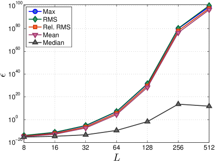
(a) All band-limits

(b) Lower band-limits

Figure 3: Average errors, for various error metrics (defined in the text), between the original and reconstructed spherical harmonic coefficients of random real spin $s=0$ functions for the numerical stability experiment explained in the text.

To examine the location of the harmonic coefficients that are poorly recovered we plot in Fig. 4 the absolute value of the original harmonic coefficients $|{f}_{{\ell}{m}}|$ and the residual error $|{g}_{{\ell}{m}}-{f}_{{\ell}{m}}|$ for one test function for various band-limits. For ${L}=16$ and ${L}=32$ (and ${L}=8$ although not shown) all harmonic coefficients are recovered accurately. For ${L}=64$ many coefficients are recovered accurately, however a small number of coefficients near the diagonal are not. Most coefficients are recovered poorly for band-limits above ${L}\simeq 128$. Errors are first introduced along the diagonal where $\ell\sim m$ and then quickly spread as $\ell$ increases.

 

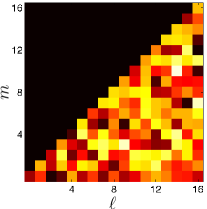
(a) Original ${L}=16$

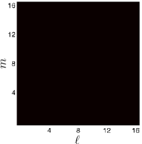
(b) Residual ${L}=16$

 

(c) Original ${L}=32$

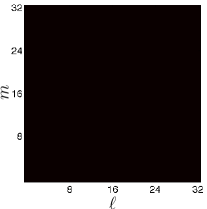
(d) Residual ${L}=32$

 

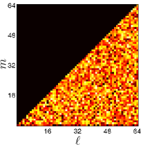
(e) Original ${L}=64$

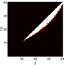
(f) Residual ${L}=64$

 

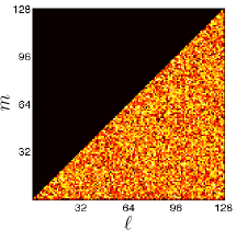
(g) Original ${L}=128$

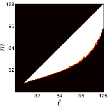
(h) Residual ${L}=128$

 

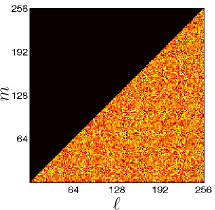
(i) Original ${L}=256$

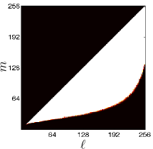
(j) Residual ${L}=256$

 

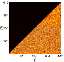
(k) Original ${L}=512$

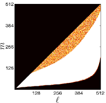
(l) Residual ${L}=512$

Figure 4: Absolute value of original spherical harmonic coefficients and residual errors for the numerical experiments explained in the text. The same colour scale is used for all plots, ranging over $[0,\sqrt{2}]$, with zero represented by dark red/black and values greater or equal to $\sqrt{2}$ by white, with intermediate values interpolated between these extremes.

The source of the numerical stability seen above has been traced to the system defined by (3.1), which is specified explicitly as a matrix system in (56). As an example, in Fig. 4.2 we show the triangular matrix ${}_{0}\mathbf{D}_{m_{0}}$ defining this system for ${L}=50$ and ${m_{0}}=38$. The matrix is extremely poorly conditioned with condition number $6\times 10^{14}$. When solving these triangular systems the increasingly large off-diagonal terms cause numerical errors to explode when recovering harmonic coefficients for low $\ell$, resulting in the error structure exhibited in Fig. 4.

We have investigated a number of numerical methods for solving these ill-conditioned systems, including a singular value decomposition (SVD) [42], preconditioning [42], the generalised minimal residual method (GMRES) [42], iterative refinements [42] and various re-normalisations; however, without success. It may indeed be possible to solve these systems using alternative numerical methods, hence we make data defining the system shown in Fig. 4.2, with the correct ${}_{0}\mbox{\boldmath${\tilde{F}}$}_{m_{0}}$ and ${}_{0}\mbox{\boldmath${\tilde{f}}$}_{m_{0}}$ vectors, available for download in case others wish to examine the system and have more success in solving it. Note that, although we have examined the numerical stability of the spin $s=0$ case only, our algorithms will also be unstable for other spin values since the corresponding linear systems that must be inverted will exhibit similar structure to the system displayed in Fig. 4.2 (i.e. increasingly large off-diagonal terms). It may be possible to rewrite the original formulation of our fast algorithms so that the equations are normalised in such a way as to avoid these ill-conditioned matrices, however we have as yet been unable to do so. Nevertheless, the conditioning of these systems is only a problem when inverting the system, thus it is only the fast forward spin spherical harmonic transform that suffers from this instability problem. The inverse spin spherical harmonic transform is likely to be accurate to high precision up to band-limits where the reduced Wigner $d$-functions can be computed accurately. However, we cannot test the inverse transform in isolation since a stable forward transform that is exact does not exist currently on the $(\theta_{t},\varphi_{p})$ grid positions defined by (45) and (46).

Figure 5: Absolute values of the ill-conditioned triangular matrix of the system that must be solved for ${L}=50$ and ${m_{0}}=38$. The matrix is extremely poorly conditioned with condition number $6\times 10^{14}$.

5 Conclusions

Algorithms have been derived to perform the forward and inverse spherical harmonic transform of functions on the sphere with arbitrary spin number. These algorithms involve recasting the spin transform on the sphere as a Fourier transform on the torus. FFTs are then used to compute Fourier coefficients, which are related to spherical harmonic coefficients through a linear transform. By recasting the problem as a Fourier transform on the torus we appeal to the usual Shannon sampling theorem to develop spherical harmonic transforms that are theoretically exact for band-limited functions, thereby providing an alternative sampling theorem on the sphere.

Previous approaches to performing spin transforms on the sphere have appealed to the spin lowering and raising operators to relate spin transforms to scalar transforms. For spin $s$ transforms based on this method the lowest computational complexity that can be attained scales as $\mathcal{O}(s{L}^{2}\log_{2}^{2}{L})$, whereas our algorithm scales as $\mathcal{O}({L}^{3})$ for arbitrary spin number $s$. Moreover, our algorithm is general in the sense that the spin number is merely a parameter of the algorithm; altering the spin number does not alter the structure of the algorithm. Furthermore, the algorithms apply for arbitrary band-limit ${L}$, whereas many other methods are restricted to band-limits that are a power of two.

Our algorithms have been implemented. The computational speed of the implementation may be improved in future by using fast discrete cosine and sine transforms in place of FFTs, although this will not alter the scaling of computation time with band-limit. Numerical tests showed that computation time scales as $\mathcal{O}({L}^{3})$, as expected. Numerical tests were also performed to assess the stability of the algorithms. Unfortunately the algorithms were found to be unstable for band-limits above ${L}\simeq 32$. The source of the instability was determined to be due to the poor conditioning of the linear system relating the Fourier and spherical harmonic coefficients. Consequently, we expect only the forward transform to be unstable and not the inverse transform, however it is not possible to verify this hypothesis since a stable forward transform that is exact (to numerical precision) does not exist currently on our pixelisation of the sphere. A number of numerical methods have been applied in an attempt to solve the ill-conditioned system but these have not proved successful.

A fast algorithm to perform a scalar spherical harmonic transform has been developed by Anthony Lasenby (private communication) in the context of geometric algebra. This algorithm shares many of the properties of the algorithms derived in this work (including, unfortunately, hints of numerical stability issues) and may simply be an alternative formulation, for the spin $s=0$ case, of the algorithms derived herein. If this indeed proves to be the case, then this alternative geometric algebra formulation may provide insight on alternative approaches to reformulate our algorithms to improve numerical stability. In ongoing work we are investigating the numerical stability problem in more detail and are attempting to renormalise or reformulate the algorithms in such a way as to eliminate this instability.

References

- [1] R. Ramamoorthi and P. Hanrahan. ACM Transactions on Graphics, 23, 4 (2004), pp. 1004.
- [2] D. L. Turcotte, R. J. Willemann, W. F. Haxby and J. Norberry. J. Geophys. Res., 86 (1981), pp. 3951.
- [3] M. A. Wieczorek. submitted to Treatise on Geophysics (2006).
- [4] M. A. Wieczorek and R. J. Phillips. J. Geophys. Res., 103 (1998), pp. 383.
- [5] J. O. Stenflo and M. Vogel. Nature, 319 (1986), pp. 285.
- [6] V. Makarov, A. Tlatov, D. Callebaut, V. Obridko and B. Shelting. Solar Physics, 198 (2001), pp. 409.
- [7] F. J. Simons, F. A. Dahlen and M. A. Wieczorek. SIAM Rev., 48, 3 (2006), pp. 504.
- [8] S. Swenson and J. Wahr. J. Geophys. Res., 107 (2002), pp. 2193.
- [9] K. A. Whaler. Geophys. J. R. Astr. Soc., 116 (1994), pp. 267.
- [10] C. H. Choi, J. Ivanic, M. S. Gordon and K. Ruedenberg. J. Chem. Phys., 111, 19 (1999), pp. 8825.
- [11] D. W. Ritchie and G. J. L. Kemp. J. Comput. Chem., 20, 4 (1999), pp. 383.
- [12] C. L. Bennett, A. Banday, K. M. Gorski, G. Hinshaw, P. Jackson, P. Keegstra, A. Kogut, G. F. Smoot, D. T. Wilkinson and E. L. Wright. Astrophys. J. Lett., 464, 1 (1996), pp. 1. astro-ph/9601067.
- [13] C. L. Bennett, M. Halpern, G. Hinshaw, N. Jarosik, A. Kogut, M. Limon, S. S. Meyer, L. Page, D. N. Spergel, G. S. Tucker, E. Wollack, E. L. Wright, C. Barnes, M. R. Greason, R. S. Hill, E. Komatsu, M. R. Nolta, N. Odegard, H. V. Peiris, L. Verde and J. L. Weiland. Astrophys. J. Supp., 148 (2003), p. 1. astro-ph/0302207.
- [14] G. Hinshaw, M. R. Nolta, C. L. Bennett, R. Bean, O. Doré, M. R. Greason, M. Halpern, R. S. Hill, N. Jarosik, A. Kogut, E. Komatsu, M. Limon, N. Odegard, S. S. Meyer, L. Page, H. V. Peiris, D. N. Spergel, G. S. Tucker, L. Verde, J. L. Weiland, E. Wollack and E. L. Wright. Astrophys. J. Supp., 170 (2007), pp. 288. astro-ph/0603451.
- [15] G. Hinshaw, J. L. Weiland, R. S. Hill, N. Odegard, D. Larson, C. L. Bennett, J. Dunkley, B. Gold, M. R. Greason, N. Jarosik, E. Komatsu, M. R. Nolta, L. Page, D. N. Spergel, E. Wollack, M. Halpern, A. Kogut, M. Limon, S. S. Meyer, G. S. Tucker and E. L. Wright. ArXiv (2008). arXiv:0803.0732.
- [16] J. Dunkley, E. Komatsu, M. R. Nolta, D. N. Spergel, D. Larson, G. Hinshaw, L. Page, C. L. Bennett, B. Gold, N. Jarosik, J. L. Weiland, M. Halpern, R. S. Hill, A. Kogut, M. Limon, S. S. Meyer, G. S. Tucker, E. Wollack and E. L. Wright. ArXiv (2008). 0803.0586.
- [17] Planck collaboration. ESA Planck blue book. Technical Report ESA-SCI(2005)1, ESA (2005). astro-ph/0604069.
- [18] S. A. Orszag. Adv. Math. Supp. Studies, 10 (1986), pp. 23.
- [19] R. K. Beatson and L. Greengard. In J. Ainsworth, J. Levesley, W. Light and M. Marletta, editors, Wavelets, multilevel methods and elliptic PDEs. Oxford University Press (1997), pp. 1–37.
- [20] B. K. Alpert and V. Rokhlin. SIAM J. Sci. Stat. Comput., 12, 1 (1991), pp. 158.
- [21] R. Suda and M. Takami. Math. Comput., 71, 238 (2002), pp. 703. ISSN 0025-5718.
- [22] K. M. Górski, E. Hivon, A. J. Banday, B. D. Wandelt, F. K. Hansen, M. Reinecke and M. Bartelmann. Astrophys. J., 622 (2005), pp. 759. astro-ph/0409513.
- [23] R. G. Crittenden and N. G. Turok. ArXiv (1998). astro-ph/9806374.
- [24] A. G. Doroshkevich, P. D. Naselsky, O. V. Verkhodanov, D. I. Novikov, V. I. Turchaninov, I. D. Novikov, P. R. Christensen and L. Y. Chiang. Int. J. Mod. Phys. D., 14, 2 (2005), pp. 275. astro-ph/0305537.
- [25] J. R. Driscoll and D. M. J. Healy. Advances in Applied Mathematics, 15 (1994), pp. 202.
- [26] D. M. J. Healy, D. Rockmore, P. J. Kostelec and S. S. B. Moore. J. Fourier Anal. and Appl., 9, 4 (2003), pp. 341.
- [27] P. Kostelec and D. Rockmore. J. Fourier Anal. and Appl., 14 (2008), pp. 145.
- [28] D. Potts, G. Steidl and M. Tasche. Linear Algebra Appl., 275/276, 1–3 (1998), pp. 433.
- [29] M. J. Mohlenkamp. A fast transform for spherical harmonics. Ph.D. thesis, Yale University (1997).
- [30] M. J. Mohlenkamp. J. Fourier Anal. and Appl., 5, 2/3 (1999), pp. 159.
- [31] M. Zaldarriaga and U. Seljak. Phys. Rev. D., 55, 4 (1997), pp. 1830.
- [32] Y. Wiaux, L. Jacques and P. Vandergheynst. J. Comput. Phys., 226 (2005), p. 2359. astro-ph/0508514.
- [33] Shannon, C. E. Proc. IRE, 37 (1949), pp. 10.
- [34] J. D. McEwen. Analysis of cosmological observations on the celestial sphere. Ph.D. thesis, University of Cambridge (2006).
- [35] T. Risbo. J. Geodesy, 70, 7 (1996), pp. 383.
- [36] J. Ivanic and K. Ruedenberg. J. Phys. Chem. A, 100, 15 (1996), pp. 6342.
- [37] M. A. Blanco, M. Flórez and M. Bermejo. J. Mol. Struct. (Theochem), 419 (1997), pp. 19.
- [38] D. A. Varshalovich, A. N. Moskalev and V. K. Khersonskii. Quantum theory of angular momentum. World Scientific, Singapore (1989).
- [39] A. F. Nikiforov and V. B. Uvarov. Classical Orthogonal Polynomials of a Discrete Variable. Springer-Verlag, Berlin (1991).
- [40] E. T. Newman and R. Penrose. J. Math. Phys., 7, 5 (1966), pp. 863.
- [41] J. N. Goldberg, A. J. Macfarlane, E. T. Newman, F. Rohrlich and E. C. G. Sudarshan. J. Math. Phys., 8, 11 (1967), pp. 2155.
- [42] W. H. Press, S. A. Teukolsky, W. T. Vetterling and B. P. Fannery. Numerical recipes in Fortran 77. Cambridge University Press, Cambridge, 2nd edition (1992).