Deep Westerbork observations of Abell 2256 at 350 MHz

Deep polarimetric Westerbork observations of the galaxy cluster Abell~2256 are presented, covering a frequency range of 325–377 MHz. The central halo source has a diameter of the order of 1.2 Mpc (18′), which is somewhat larger than at 1.4 GHz. With $\alpha=-1.61\pm 0.04$, the halo spectrum between 1.4 GHz and 22.25 MHz is less steep than previously thought. The centre of the ultra steep spectrum source in the eastern part of the cluster exhibits a spectral break near 400 MHz. It is estimated to be at least 51 million years old, but possibly older than 125 million years. A final measurement requires observations in the 10–150 MHz range. It remains uncertain whether the source is a radio tail of Fabricant galaxy 122, situated in the northeastern tip of the source. Faraday rotation measure synthesis revealed no polarized flux at all in the cluster. The polarization fraction of the brightest parts of the relic area is less than 1%. The RM-synthesis nevertheless revealed 9 polarized sources in the field enabling an accurate measurement of the Galactic Faraday rotation ($-33\pm 2$ rad m^-2 in front of the relic). Based on its depolarization on longer wavelengths, the line-of-sight magnetic field in relic filament G is estimated to be between 0.02 and 2 $\mu$G. A value of $0.2$ $\mu$G appears most reasonable given the currently available data.

1 Introduction

Abell 2256 is one of the most massive clusters in the nearby universe. It has been studied extensively at X-ray, optical, and radio wavelengths. The galaxies associated with the cluster can be divided into three distinct populations, based on their kinematics (Berrington et al. 2002). X-ray images of the cluster reveal several substructures superimposed on a fairly smooth main source (Sun et al. 2002; Molendi et al. 2000; Roettiger et al. 1995; Briel et al. 1991), indicating that Abell 2256 is currently involved in a major merger event.

The cluster has some interesting radio properties. It contains the largest number of head-tail galaxies of all known clusters (Miller et al. 2003). One of them has a straight, almost 1 Mpc long tail. There is a complex steep spectrum source in the eastern part of the cluster (Röttgering et al. 1994; Masson & Mayer 1978; Bridle et al. 1979). The cluster is embedded in a large, diffuse, unpolarized radio halo (Bridle & Fomalont 1976; Kim 1999; Clarke & Enßlin 2006) that dominates the total flux at decametric wavelengths (Costain et al. 1972). The most striking feature is the large, bright relic source in the northwestern part of the cluster. Although it is 20–40% linearly polarized at 1.4 GHz (Bridle et al. 1979; Clarke & Enßlin 2006), Jägers (1987) did not detect any linear polarization at 608.5 MHz, establishing a $3\sigma$ upper limit of 20% fractional polarization.

There are strong indications that relic sources are caused by large scale structure formation (LSS) shocks compressing buoyant bubbles of magnetized plasma that have been emitted by active galactic nuclei in the past (Enßlin & Gopal-Krishna 2001; Enßlin & Brüggen 2002; Brüggen 2003; Hoeft & Brüggen 2007). Shortly after their injection into the intergalactic medium (IGM), these bubbles have faded beyond detection limits due to synchrotron losses and adiabatic expansion. An encounter with a LSS shock wave would then compress the plasma, increasing and aligning the magnetic field, and accelerate the electrons to energies enabling synchrotron emission at radio wavelengths. This model explains both the high fractional polarization that is usually observed in these relic sources and their peripheral position.

De Bruyn & Brentjens (2005) have discovered several highly polarized structures in the direction of the Perseus cluster that were tentatively attributed to the cluster itself. Some of the structures resembled buoyant bubbles in the IGM of the Perseus cluster, while others looked like long, straight shock fronts. One of these ”fronts” was located at the western edge of the cluster at the interface to the Perseus-Pisces supercluster, exactly where such shocks are expected to occur. However, these structures have not been detected in Stokes $I$, hence the exact fractional polarization is unknown. The two most likely reasons for the non-detection of Stokes $I$ are:

• The sources are highly polarized and the Stokes $I$ brightness is below the confusion limit of the Westerbork Synthesis Radio Telescope (WSRT) in these observations;

• The structures have Stokes $I$ structure at much larger scales than the Stokes $Q$ and $U$ structure, rendering it invisible at even the shortest interferometer baseline.

The latter situation is common in the Galactic synchrotron foreground (Wieringa et al. 1993). A Galactic interpretation can therefore not be ruled out. However, Govoni et al. (2005) have observed similar structures in Stokes $I$ near Abell~2255 with the VLA at 1.4 GHz. Abell 2256 was chosen to search for similar objects because of its proximity, its dynamic nature, its relic source, and its moderate Galactic latitude of $32\degr$.

Wide field polarimetric images with noise levels well below 1 mJy beam^-1 are required in order to detect such sources. Additionally, the images can be used to find more polarized background sources in order to establish the Galactic contribution to the Faraday rotation measure (RM) towards the cluster, and to determine the decline of the fractional polarization with increasing wavelength, enabling a measurement of the thickness of the relic sources in RM-space.

The spectrum of the diffuse halo source has been rather uncertain. Bridle et al. (1979) favoured a spectral index ($S_{\nu}\propto\nu^{\alpha}$) of $\alpha<-1.2$ between 610 and 1415 MHz and $\alpha\approx-1.8$ between 151 and 610 MHz, based on maps where the halo was only marginally detected. More recently Clarke & Enßlin (2006) determined the 1.4 GHz halo flux in more sensitive VLA D observations, but could not derive the spectrum of the halo because of the large uncertainties in the halo flux measurements available to them. They assumed that $-1.7\lesssim\alpha\lesssim-1.25$. Kim (1999) determined that $\alpha=-2.04\pm 0.04$, but this estimate was partly based on an erroneous value of the total cluster flux at 81.5 MHz, and partly on maps in which the halo was only marginally detected. New measurements of the 351 MHz flux of the halo and the entire cluster are presented in Sect. 4. These values are combined with corrected literature values in order to obtain accurate spectra for the cluster as a whole and the diffuse halo source itself.

The redshift of Abell~2256 is 0.058 (Berrington et al. 2002). Assuming $H_{0}=71$ km s^-1 Mpc^-1 (Spergel et al. 2003), 1′ on the sky corresponds to 67.8 kpc at the cluster.

2 Observations

The observations were conducted with the Westerbork Synthesis Radio Telescope, which consists of fourteen parallactic 25 m dishes on an east-west baseline and uses earth rotation to fully synthesize the uv-plane in 12 h. There are ten fixed dishes (RT0–RT9) and four movable telescopes (RTA–RTD). The distance between two adjacent fixed telescopes is 144 m.

The data set consists of two observing sessions of 12 h each. The first during the night of May 17/18 2004 with RT9–RTA = 36 m and the second during the night of May 18/19 with RT9–RTA = 72 m. The distances between the movable dishes were kept constant (RTA–RTB = RTC–RTD = 72 m, RTB–RTC = 1224 m). The uv-plane is therefore sampled at regular intervals of 36 m out to the longest baseline of 2736 m. Only the zero spacing is missing. The regular interval causes a grating ring with a radius of 80$\arcmin$ at 350 MHz. At this frequency the $-5$ dB and $-10$ dB points of the primary beam are at radii of $70\arcmin$ and $120\arcmin$ respectively. The observations are sensitive to angular scales up to $90\arcmin$ at a resolution of $67\arcsec$ full width at half maximum (FWHM).

The eight frequency bands were each 10 MHz wide and centred at 319, 328, 337, 346, 355, 365, 374, and 383 MHz. The WSRT is equipped with linearly polarized feeds for this frequency range. The $x$ dipole is oriented north-south and the $y$ dipole east-west. The correlator produced 64 channels in all four cross correlations for each band with an integration time of 30 s. The on-line system applied a uniform lag-to-frequency taper. A Hanning lag-to-frequency taper was applied off-line, effectively halving the frequency resolution. The pointing centre and phase centre were at the optical centre of the cluster at $\alpha=17^{\mathrm{h}}03^{\mathrm{m}}45^{\mathrm{s}}$, $\delta=+78\degr 43\arcmin 00\arcsec$ (J2000.0).

The observations were bracketed by two pairs of calibrators, each consisting of one polarized and one unpolarized source. 3C~295 and the eastern hot spot of DA~240 were observed before Abell 2256 and PSR~B1937+21 and 3C~48 afterwards.

The theoretical image noise in one Hanning tapered channel of a single 12 h observation at 350 MHz is about 1.56 mJy beam^-1 (uniform weighting). Band 1 was unusable on the second night due to a polarization calibration problem. Band 4 suffered from a strange, broad band interference on the shorter baselines and was therefore discarded. Band 8 (383 MHz) was unusable in both nights due to man made interference. The four lowest and four highest channels of the remaining bands were discarded. Only the odd channels were selected because they are linearly dependent on the even channels due to the Hanning taper. In the remaining 28 channels per band, 60% of the data was usable. The expected thermal noise level in the integrated polarization maps is therefore 1.56 mJy beam^-1/$\sqrt{2\times 28\times 5\times 0.6}\approx 0.12$ mJy beam^-1. This level can not be reached in the total intensity maps because they are confusion limited at approximately 0.3 mJy beam^-1 at this frequency and resolution (Morganti 2004).

3 Data reduction

Flagging, imaging, and self calibration were performed with the AIPS++ package (McMullin et al. 2004). System temperature corrections, flux scale calibration, polarization calibration, ionospheric Faraday rotation corrections, and deconvolution were performed with a calibration package written by the author and based on the AIPS++ and CASA libraries.

3.1 System temperatures

The system temperature readings of the 36 m observing session were unfortunately unusable due to problems with the preparation of the telescope for the observations. The system temperature readings of the 72 m session were usable, but had large spikes caused by RFI. The system temperature corrections were therefore only applied to the 72 m data, not to the 36 m data. The 72 m system temperatures were filtered using a median window with a total width of 20 minutes, which was very effective in mitigating the effect of short bursts of RFI. The difference between the $x$ and $y$ system temperatures of some bands in several antennas was of the order of 30–50 K, although for most band/antenna combinations it was less than 5 K. Because of the lack of system temperature data in the 36 m session, the 72 m data were used to determine the flux scale of the point source model used for self calibration. The 36 m data were later tied to the same flux scale in order to combine them with the 72 m data for the Stokes $I$ image. The 36 m data were not used for polarimetry because there was small, but significant polarization leakage even after cross-calibration. This may have been caused by temporal variations in the difference in the system temperatures between the $x$ and $y$ receptors during the observation.

3.2 Bandpass- and polarization calibration

The flux scale and polarization leakages were calibrated simultaneously using the unpolarized calibrator sources 3C 295 and 3C 48. The Measurement Equation (Sault et al. 1996) for the visibility on the baseline $i$–$j$ at a certain frequency is given by

$$\@tens{\tilde{V}}_{ij}=\@tens{J}_{i}\@tens{V}_{ij}\@tens{J}_{j}^{\dagger},$$ (1)

where

$$\@tens{V}_{ij}=\left(\begin{array}[]{cc}<xx>&<xy>\\ <yx>&<yy>\end{array}\right)_{ij}$$ (2)

represents the pure sky visibilities in terms of the cross correlations between the $x$ and $y$ receptors of the antennae in the baseline, $\@tens{J}_{i}$ and $\@tens{J}_{j}$ are the Jones matrices describing the properties of the antennae, and $\@tens{\tilde{V}}_{ij}$ is the observed coherency matrix. The $\dagger$ denotes Hermitian matrix transposition.

The fluxes of the calibrator sources were computed using the expressions and coefficients given in Perley & Taylor (1999), which extends the Baars et al. (1977) flux scale to lower frequencies. Because each channel is individually tied to this flux scale, all sources appear in the images with their true spectral indices.

The on-axis and off-axis polarization leakages at the WSRT are strongly frequency dependent with a period of the order of 17 MHz. The leakage amplitude can increase from almost negligible to 1.5% and decrease back to negligible over a frequency interval of approximately 8.5 MHz. It was therefore necessary to solve for all elements of the Jones matrices for each channel individually. The phases of the diagonal elements of the Jones matrix of RT1 were fixed at 0. The remaining $x$–$y$ phase difference,

$$\delta_{xy}=\tan^{-1}\frac{V}{U}+n\pi,$$ (3)

where $n$ is an integer, rotates Stokes $U$ into Stokes $V$. It is fortunately fairly constant across a 10 MHz band. Equation (3) has only two unique solutions: one when $n$ is even, the other when $n$ is odd. One solution rotates the $(U,V)$ vector to positive $U$, the other to negative $U$. In order to select the correct solution, one only requires the sign of the RM of the calibrator sources. The (sinusoidal) Stokes $U$ spectrum is shifted by 90° towards smaller $\lambda^{2}$ with respect to the Stokes $Q$ spectrum if the RM is positive and 90° in the opposite direction if it is negative.

PSR 1937+21 and the eastern hot spot of DA 240 both have a positive RM. According to Tsien (1982) the RM of DA 240 is +2.4 rad m^-2 (no error quoted). According to A.G. de Bruyn, the RM of DA 240 plus a minimal ionosphere should be $+3.7\pm 0.5$ rad m^-2. Using the low frequency front ends of the WSRT, he found that the RM of the pulsar, also without correcting for the ionospheric RM, is $+8.5\pm 0.5$ rad m^-2 (private communication).

Table 1: Faraday rotation measures and position angles (north through east) at $\lambda^{2}=0$ for the polarized calibrator sources.

Source	Rotation measure	Position angle
	(rad m-2 )	(°)
PSR~1937+21	$+7.86\pm 0.20$	$291.4\pm 1.1$
DA~240	$+3.33\pm 0.14$	$122\ \ \ \pm 3$

The most accurate rotation measures for these objects to date are listed in Table 1. They were obtained after correcting for ionospheric Faraday rotation using the procedure outlined in Sect. 3.4. Because the shorter spacings were all affected by solar interference, the polarization angle at each frequency was computed based on the average visibility of all spacings larger than 700 $\lambda$.

3.3 Phase calibration

After the data were corrected for the more or less time independent effects described in the previous section, three phase-only self calibration iterations were performed on the 72 m data set (Pearson & Readhead 1984). The sky model consisted of a list of 103 bright point source components with accurate positions and $I$, $Q$, $U$, and $V$ fluxes for each channel, supplemented with a grid of 15525 CLEAN components (Högbom 1974) in Stokes $I$. The CLEAN model was given a spectrum proportional to $\nu^{-1}$. Both models were updated after every self calibration step.

The initial models were obtained by:

1. Making an image of a channel close to 350 MHz with all baselines $>600\ \lambda$;

2. Identifying all point sources brighter than 30 mJy beam^-1;

3. Solving for positions of all 103 sources in band 5 in the uv-plane (band 5 had very little RFI);

4. Solving for $I$, $Q$, $U$, and $V$ of all 103 point sources for each channel in the uv-plane;

5. Solving for phases using the point source model and all baselines $>600\ \lambda$ ;

6. Correcting the visibilities for these phases;

7. Subtracting the point source model from the visibilities;

8. Making (residual) Stokes $I$ images of all usable channels and CLEAN them;

9. Constructing the CLEAN model by averaging the CLEAN models of all channels.

One self calibration iteration consisted of the following steps:

1. Adding the point source model to the visibilities

2. Solving for phase corrections using the point source model and the CLEAN model on all baselines $>200\ \lambda$;

3. Solving for point source model fluxes;

4. Subtracting the point source model from the visibilities;

5. Making (residual) Stokes $I$ images of all usable channels and CLEAN them;

6. Constructing the CLEAN model by averaging the CLEAN models of all channels.

The final CLEAN model was the average of the CLEAN models of individual channel maps that were produced after subtracting the point source component model. This lead to a very detailed and smooth representation of the extended emission in the CLEAN model.

After the self calibration, data points were flagged if the absolute value of the residual visibility (corrected data minus model data) was larger than 5 times the root mean square (RMS) amplitude of the residuals for that band and baseline.

3.4 Ionospheric Faraday rotation

The ionospheric Faraday rotation at the WSRT is typically between 0.2 and a few rad m^-2. Daytime values of 5 rad m^-2 are possible during solar maximum. A difference of 2 rad m^-2 in ionospheric Faraday depth corresponds to a change in polarization angle of $>100\degr$ at the lowest frequency ($\approx 315$ MHz). The polarized calibrator sources showed a difference of up to 20° in their polarization angle between the 36 m and 72 m sessions at the lowest frequencies, even though they were observed at the same time of the day on consecutive days. It was therefore necessary to compensate for the ionospheric RM in order to avoid depolarization.

Erickson et al. (2001) showed that a simple ionospheric model fed with data from dual band GPS receivers installed at the VLA could predict the ionospheric rotation measure in most circumstances to better than 0.04 rad m^-2. Sometimes, however, they observed an unexplained discrepancy of the order of 30° between the predicted and observed polarization angle of PSR~1932+109. This corresponds to a mismatch in RM of approximately 0.6 rad m^-2.

Because there are only very few lines of sight through the ionosphere with the single dual band GPS receiver installed at the WSRT, the ionospheric Faraday rotation was computed using global GPS total ionospheric electron content (TEC) data and an analytical model of the geomagnetic field. The GPS-TEC data were provided by the Center for Orbit Determination in Europe (CODE) of the Astronomical Institute of the university of Bern, Switzerland. The geomagnetic field was computed using the US/UK World Magnetic Model (WMM) (Macmillan & Quinn 2000), while the ionosphere was modelled as a spherical shell with a finite thickness and uniform density at an altitude of 350 km above mean sea level. The geomagnetic field parallel to the line of sight was evaluated at the points where the line of sight from the WSRT towards Abell~2256 pierced through the model ionosphere. The TEC data are published for all even UTC hours. The expected uncertainty in RM towards Abell 2256, based on the TEC RMS uncertainty published by CODE, is typically 0.07–0.1 rad m^-2 for each data point during the observations.

The ionospheric RM was also tracked using 6C~B165001.3~+791133, a polarized source at 53$\arcmin$ from the phase centre. Its polarized flux is about 15 mJy at 350 MHz, yielding an apparent polarized flux of approximately 10.1 mJy after primary beam attenuation. The total Faraday depth as a function of time is

$$\phi_{\mathrm{tot}}(t)=\phi_{\mathrm{src}}+\phi_{\mathrm{ion}}(t),$$ (4)

where $\phi_{\mathrm{ion}}(t)$ is the time dependent ionospheric Faraday rotation and $\phi_{\mathrm{src}}$ is the constant contribution of 6C B165001.3 +791133. Based on the thermal noise, $\phi_{\mathrm{tot}}$ could be estimated with an accuracy of approximately 0.26 rad m^-2 every two hours. This translates to a 1$\sigma$ error in the polarization plane of approximately $13\degr$ at 324 MHz.

Figure 1: Ionospheric RM as predicted by global GPS-TEC data and the US/UK World Magnetic Model. The dashed lines indicate the $\pm 1\sigma$ predicted TEC/WMM rotation measures, interpolated between the 2 h intervals at which the data are published. The points with error bars are observed RMs of 6C B165001.3 +791133, shifted up by 27.0 rad m^-2. The horizontal axis is the time in hours since May 19 2004, 00:00 UTC.

Figure 1 compares the observed changes in ionospheric Faraday rotation with the predicted ionospheric RM based on GPS-TEC/WMM data. The uncertainty in the GPS-TEC/WMM rotation measures is based on the RMS error in the TEC along the given line-of-sight. Uncertainties in the geomagnetic field are not incorporated. After discarding the outlier directly after sunrise, $\phi_{\mathrm{src}}=-27.0\pm 0.1$ rad m^-2.

The Abell 2256 visibilities were corrected for the ionospheric Faraday rotation after instrumentally polarized point sources were subtracted in order to prevent residuals of these sources due to distortion of their PSF by the ionospheric Faraday rotation correction.

3.5 Imaging

The final dirty channel images in all Stokes parameters and the corresponding point spread functions (PSFs) were created from the corrected visibilities after subtracting the instrumentally polarized point sources. The uv-plane was uniformly weighted. Because of a fractional bandwidth of 15%, the area under the main lobe of the PSF at the lowest frequency is 30% larger than at the highest frequency, hence a Gaussian taper was applied to the uv-plane before Fourier transforming in order to convolve the images to a common resolution of $67\arcsec$ FWHM. All maps are in North Celestial Pole (NCP) projection. The dirty maps are 2048$\times$2048 pixels large, with a pixel size of $15\aas@@fstack{\prime\prime}6$. The central 1024$\times$1024 pixels of the dirty images were deconvolved using a Högbom CLEAN (Högbom 1974).

While deconvolving the Stokes $I$ channel images, CLEAN was constrained to only search for components at certain pixel positions (the mask). The mask was obtained by averaging all channel maps of a previous deconvolution, selecting all pixels where Stokes $I$ was larger than some threshold, and expanding the mask to include all pixels where at least one of its eight neighbours was part of the mask. The threshold level was lowered after each self calibration iteration. The final threshold level for the mask was 1.5 mJy beam^-1. The loop gain was set to 0.3 and the CLEAN was stopped whenever either 15000 iterations were performed or the maximum residual in the area where CLEAN components were allowed was less than 0.5 mJy beam^-1. This is roughly one third of the thermal noise level in the individual channel maps. It was necessary to deconvolve so deep into the noise of individual channels in order to obtain the highest possible dynamic range in the average of 116 channel maps. The CLEAN models were added to the residual images using a circular Gaussian restoring beam with a FWHM of 67″. At this declination, the north-south to east-west ratio of the untapered WSRT PSF is 1.02. The use of a circular restoring beam is justified in this case because of the strong, circular uv-plane taper that was applied.

After deconvolution, the channel maps were corrected for the total power primary beam of the WSRT, which can be approximated by

$$G(\nu,\gamma)=\cos^{6}{k\nu\gamma},$$ (5)

where $\nu$ is the frequency in Hz, $\gamma$ is the angular distance from the pointing centre in radians, and $k=6.6\times 10^{-8}$ s is a constant, namely the light crossing time across a 19.8 m aperture, which is roughly the effective diameter of a WSRT dish in this frequency band (25 m dish, 63% effective surface area). Finally, the best 116 channel maps were averaged.

The deconvolution of the Stokes $Q$ and $U$ maps was unconstrained. The CLEAN was considered complete after 5000 iterations or if the largest residual on the inner 1024$\times$1024 pixels was less than 1 mJy beam^-1. These images were also corrected for the primary beam. Unfortunately the 36 m observing session suffered from residual polarization leakage due to gain variations during the observations. It turned out to be difficult to obtain correct gain solutions, and system temperature data were corrupted. Therefore the polarization images were created using only the 72 m spacing.

3.6 RM-synthesis

The low frequency and high fractional bandwidth of these observations required RM-synthesis (Brentjens & de Bruyn 2005) in order to avoid bandwidth depolarization. Images were created for Faraday depths of -800 to +800 rad m^-2 in steps of 2 rad m^-2.

Off-axis instrumental polarization was not corrected because it is limited to very specific Faraday depths after RM-synthesis. In the case of the WSRT the off-axis polarization consists of two components: a largely frequency independent offset and a frequency- and direction dependent oscillation with a period of 17 MHz. After RM-synthesis, the offset ends up at $\phi=0$ rad m^-2 and the 17 MHz oscillation at $|\phi|\approx 44$ rad m^-2 (near 350 MHz). The sign of $\phi$ depends on the position angle with respect to the pointing centre.

The noise level in the images ranges from 0.31 mJy beam^-1 near 0 rad m^-2 to the thermal noise level of 0.12 mJy beam^-1 for Faraday depths $|\phi|>300$ rad m^-2. The polarization images were corrected for the total intensity primary beam of the WSRT using Eq. (5) before the RM-synthesis was applied.

4 Total intensity

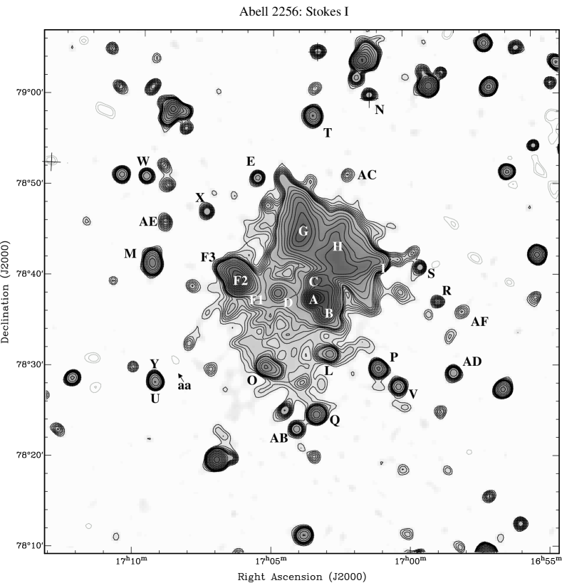
Figure 2: Total intensity image of Abell~2256 observed with the WSRT in 2004. Contour levels are at ($-4$, $-3$, 3, 4, 5, 6, 7, 8, 9, 10, 14, 20, 28, 40, 56, 80, 113, 160, 226, 320)$\times$0.6 mJy beam^-1. The beam is a circular Gaussian with a FWHM of $67\arcsec$. Crosses mark locations where point source components have been subtracted. The average frequency of this multi frequency synthesis map is 351 MHz.

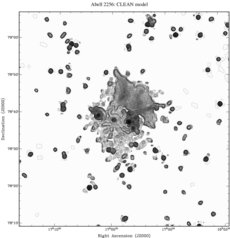
Figure 3: The average CLEAN model convolved with a circular Gaussian beam with a FWHM of 26″. The contours are at ($-4$, $-3$, 3,4, 5, 6, 7, 8, 9, 10, 14, 20, 28, 40, 56, 80, 113, 160, 226, 320)$\times$91 $\mu$Jy beam^-1.

Figure 2 shows the central square degree of the final Stokes $I$ image. The average frequency of the combined map is 351 MHz and the integrated bandwidth is 43 MHz spread over 52.5 MHz. The noise level near the centre of the map is approximately 0.6 mJy beam^-1, dominated by residual calibration problems. The dynamic range of the full map (brightest source:central noise level) is of the order of 3000:1. Sources are labelled according to Bridle et al. (1979), including the extension by Röttgering et al. (1994).

Figure 3 displays a mildly super-resolved map of the same region. It was obtained by convolving the CLEAN model with a circular Gaussian beam of $26\arcsec$ FWHM. This map reproduces the filamentary structure seen in the relic area by (Clarke & Enßlin 2006). The halo itself appears to exhibit filamentary structure too.

Except for source AA, all sources mentioned in Röttgering et al. (1994) were detected. For source AA, they list a total flux of 2.8$\pm$0.3 mJy at 1446 MHz. Although they mention the source has a flux of 8 mJy at 327 MHz, it is not visible in their 327 MHz map. H.J.A. Röttgering agrees that their flux estimate of source AA at 327 MHz is caused by an error in the flux estimation procedure (private communication). My non-detection gives a 3$\sigma$ upper limit of 1.8 mJy at 351 MHz. The source is also invisible in recent WSRT observations at 150 MHz, yielding a 3$\sigma$ upper limit of 12 mJy (H.J.A. Röttgering, private communication). The spectral index $\alpha$ ($S_{\nu}\propto\nu^{\alpha}$) between 351 MHz and 1446 MHz must therefore be larger than 0.3.

The remainder of this paper focuses on the diffuse halo emission that pervades the cluster, the steep spectrum source F, and the relic area containing filaments G, H, and the tail of source C. The complex involving sources A and B will not be discussed.

4.1 Halo flux at 351 MHz

The largest structure visible in Fig. 2 is the diffuse emission approximately centred on the X-ray source at J2000 position 17^h4^m2^s +78°37′55″ (Ebeling et al. 1998), and extending to the sources F, O, L, H, and G. This halo source has been described by several authors (Bridle & Fomalont 1976; Bridle et al. 1979; Kim 1999; Clarke & Enßlin 2006). It is considered to be the main contributor to the total flux of the cluster at decametric wavelengths (Costain et al. 1972).

The total flux of the halo at 351 MHz was estimated using the data selection from Fig. 2. The flux estimate is complicated by several bright, extended radio sources in the cluster, which have to be subtracted first. Because of their complex nature, the sources were subtracted in the image plane. Two different approaches were used to estimate the halo flux in the area enclosed by the thick, grey contour in Fig. 4.

In the first approach the CLEAN model was set to zero inside the areas enclosed by the white contours in Fig. 4. The model was subsequently convolved with a circular Gaussian of $67\arcsec$ FWHM and added to the residual image. Let $\Phi$ be the set of $n_{\mathrm{\Phi}}$ pixels enclosed by the grey contour and let $\mu$ be the set of $n_{\mathrm{\mu}}$ pixels enclosed by both the grey contour and a white contour. The integrated halo flux is then the sum of all pixels in $\Phi$ that are not in $\mu$, multiplied by $\frac{n_{\mathrm{\Phi}}}{n_{\mathrm{\Phi}}-n_{\mathrm{\mu}}}$ and divided by the volume of the $67\arcsec$ circular Gaussian, which results in a flux of $696\pm 8$ mJy. This is most likely a low estimate, because the sources A, B, C, D, F, and the eastern parts of G and H, are situated predominantly in the brighter parts of the halo. The fainter south-eastern part of the halo therefore has a relatively large influence on the sum.

In the second approach, the CLEAN model pixels in $\mu$ were not set to zero, but were replaced by a radial basis function interpolation (Carr et al. 2001) of the pixels that constitute the border of the areas enclosed by the white contours. This interpolated model was convolved with a circular Gaussian of $67\arcsec$ FWHM and added to the residual image. The result is shown in Fig. 4. The interpolation works extremely well for sources up to the size of source F. The interpolation of the vast area of sources A, B, C, G, and H is less successful and appears a bit too faint in the area of A, B, and C, and a bit too bright in the area of G and H. The total flux was computed by adding the values of all pixels of the restored image that are in $\Phi$ and dividing by the volume of the $67\arcsec$ circular Gaussian. The result of $831\pm 10$ mJy is probably a somewhat high estimate because of the relatively high interpolated surface brightness of the relic area, which lacks the filamentary structure seen in the rest of the halo. The total halo flux is therefore estimated at $0.76\pm 0.07$ Jy, which is the average of the two approaches. The uncertainty is mainly systematic.

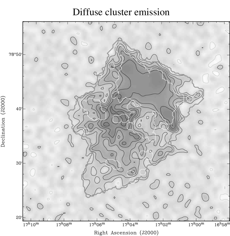
Figure 4: The radio emission of the halo of Abell~2256 at 351 MHz. The contours are drawn at 1, 2, 3, 4, 5, and 6 mJy beam^-1 of $67\arcsec$ FWHM. In the areas enclosed by the white contours, the surface brightness was replaced by a radial basis function interpolation of the fluxes along the white contours.

4.2 Radio spectrum

The integrated radio flux of the entire cluster (halo, relic, and discrete sources combined) was determined from Fig. 2 by measuring the integrated flux within a circle centred at the optical centre of Abell 2256 at J2000.0 position $\alpha=17^{\mathrm{h}}03^{\mathrm{m}}45^{\mathrm{s}}$, $\delta=+78\degr 43\arcmin 00\arcsec$. The radius of the circle was determined using Fig. 5. The derivative of the integrated flux within a circle with respect to the radius of the circle is fairly high at small radii, where there is significant cluster emission. At radii $>5\arcmin$, the derivative drops sharply and settles at a more or less constant value at a radius of $10\arcmin$, which was therefore assumed to be the cluster radius. The integrated flux within $10\arcmin$ of the optical cluster centre is $3.51\pm 0.06$ Jy at a frequency of 351 MHz.

Table 2 lists flux estimates for the halo as well as the entire cluster including relics, head-tail galaxies, and background sources. All fluxes have been converted to the flux scale of Perley & Taylor (1999) using the flux of Cas A, taking its secular variation into account. At frequencies above 408 MHz, this flux scale is equivalent to the Baars et al. (1977) flux scale.

Note that the flux at 81.5 MHz is twice the flux from Branson (1967), as suggested by Masson & Mayer (1978). The flux measurements from Kim (1999) have been read off Fig. 3 of that paper. The two measurements of the total cluster flux at 408 MHz and 1420 MHz appear to be systematically lower than all other cluster flux observations. It was therefore decided not to use these fluxes to determine the average spectra of Abell 2256 (halo plus relic and discrete sources) and its halo.

The fluxes from Table 2 are plotted in Fig. 6. It is assumed that the cluster flux can be modelled as the sum of two spectral components, each with a constant spectral index between 22.25 MHz and 2695 MHz:

$$S(\nu)=S_{\mathrm{H,100}}\left(\frac{\nu}{100\ \mathrm{MHz}}\right)^{\alpha_{\mathrm{H}}}+S_{\mathrm{R,100}}\left(\frac{\nu}{100\ \mathrm{MHz}}\right)^{\alpha_{\mathrm{R}}},$$ (6)

where the first term is due to the halo and the second term is due to all other sources (relic and discrete sources). Fitting Eq. (6) to the total cluster fluxes, assuming uncertainties of 10% for all flux points with unknown errors, yields

$$\begin{array}[]{lcrcl}S_{\mathrm{H,100}}&=&6.0&\pm&2.1\ \mathrm{Jy}\\ \alpha_{\mathrm{H}}&=&-1.65&\pm&0.22\\ S_{\mathrm{R,100}}&=&6.8&\pm&1.8\ \mathrm{Jy}\\ \alpha_{\mathrm{R}}&=&-0.72&\pm&0.07.\end{array}$$ (7)

This suggests that the spectrum of the halo may be less steep than the estimates by Costain et al. (1972) ($-1.9$ between 22.25 MHz and 81.5 MHz) and Bridle et al. (1979) ($-1.8$ between 151 MHz and 610 MHz).

As Fig. 6 shows, the halo spectrum lies much closer to the halo fluxes derived in this paper and by Clarke & Enßlin (2006) than to the flux estimates by Bridle et al. (1979) and Kim (1999). These sets of estimates are in fact mutually inconsistent. The reason is that the maps in this paper and the maps in Clarke & Enßlin (2006) are much deeper and detect the halo source over a larger area than Bridle et al. (1979) and Kim (1999). The halo appears to be roughly circular with a diameter of 12$\aas@@fstack{\prime}$2 at 1369 MHz (Clarke & Enßlin 2006). The map in Fig. 4 shows that the halo is approximately square with a triangular south-eastern extension at 351 MHz. The sides of the square are $18\arcmin$ long at 1 mJy beam^-1 and $13\arcmin$ at 3 mJy beam^-1. The sides of the triangular extension are $6\arcmin$ long at 1 mJy beam^-1. The halo is only marginally detected in the 610 MHz map of Bridle et al. (1979) and at the noise level in their 1415 MHz map. They estimated its diameter at $9\arcmin$ to $10\arcmin$. Kim (1999) estimates the halo size slightly larger ($13\arcmin\times 10\arcmin$), but the halo is still only marginally above the noise in the 1420 MHz map presented in that paper. It is therefore not surprising that the halo flux estimates in these papers were relatively low.

Using the 1369 MHz halo flux of Clarke & Enßlin (2006) and the 351 MHz flux derived above, the spectral index of the halo is estimated at $-1.5\pm 0.2$ between these frequencies. Including the 351 MHz and 1369 MHz halo fluxes in a joint fit with the total cluster flux points gives much better constrained values between 22.25 MHz and 2695 MHz:

$$\begin{array}[]{lcrcl}S_{\mathrm{H,100}}&=&5.9&\pm&0.3\ \mathrm{Jy}\\ \alpha_{\mathrm{H}}&=&-1.61&\pm&0.04\\ S_{\mathrm{R,100}}&=&6.7&\pm&0.2\ \mathrm{Jy}\\ \alpha_{\mathrm{R}}&=&-0.72&\pm&0.02.\end{array}$$ (8)

The reduced $\chi^{2}$ of the fit is 0.23, indicating that at least some fluxes in Table 2 are more accurate than stated.

Figure 5: The solid line is the total 351 MHz radio flux in Jy within a circle centred on the optical cluster centre as a function of the radius of the circle in arcminutes. The dotted line is the derivative with respect to the radius.

Table 2: Flux measurements for Abell 2256.

$\nu$	$S$		C/H	Fit	Reference
(MHz)	(Jy)
22.25	100 $\pm$	32	C	+	C72
38	41 $\pm$	6	C	+	W66
81.5	17 $\pm$	2	C	+	B67/M78
151	8.1 $\pm$	0.8	C	+	M78
351	3.51 $\pm$	0.06	C	+	B08
408	2.4 $\pm$	0.24	C	$-$	K99
610	2.165 $\pm$	…	C	+	B76
1410	1.13 $\pm$	…	C	+	B76
1420	0.75 $\pm$	0.11	C	$-$	K99
2695	0.57 $\pm$	0.16	C	+	O75
2695	0.666 $\pm$	…	C	+	H78
151	1.5 $\pm$	…	H	$-$	B79
351	0.76 $\pm$	0.07	H	+	B08
610	0.1 $\pm$	…	H	$-$	B79
1369	0.103 $\pm$	0.020	H	+	C06
1415	0.02 $\pm$	…	H	$-$	B79
1420	0.03 $\pm$	0.009	H	$-$	K99

Figure 6: Spectra of the entire cluster and its two spectral components representing the halo and the rest of the cluster (see Eq. (6)). The labels indicate the source paper for the data points. Refer to Table 2 for details on the flux values. The solid lines represent the sum of the two spectral components as computed by Eq. (6). The dashed lines represent the individual spectral components. The long dashes represent the halo model and the short dashes the rest of the cluster. The thin curves show the spectral fit of Eq. (6) to the total cluster flux. The thick curves show the fit where the B08 and C06 fluxes of the halo have been used as extra condition equations on the spectral component of the halo. The total cluster fluxes of both solutions virtually overlap.

4.3 Source F

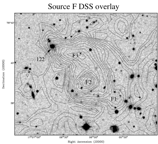
Figure 7: Palomar DSS blue map of source F overlaid with 351 MHz Stokes $I$ contours. The contour levels are: 0.2, 0.28, 0.4, 0.56, … mJy beam^-1, with a circular Gaussian beam of $26\arcsec$ FWHM. The role of Fabricant galaxy 122 is discussed in the text.

Figure 8: Radio spectrum of source F2. The labels of the data points indicate its source (see Table 2). The error bar on the 151 MHz point indicates the uncertainty in the extrapolation of the 351 MHz flux with the 338/365 MHz spectral index to 151 MHz rather than the uncertainty in the estimate by Bridle et al. (1979).

Source F is a bright, ultra steep spectrum source (Masson & Mayer 1978; Bridle et al. 1979; Röttgering et al. 1994). An optical image from the Palomar Digital Sky Survey, overlaid with the Stokes $I$ contours at 351 MHz is shown in Fig. 7. Source F has three components: F1 (southwest), F2 (central), and F3 (northeast). Bridle et al. (1979) suggested that because the spectral index between 1415 MHz and 610 MHz of the entire source is rather constant, F1, F2, and F3 could be physically related. They suggested that the entire source is the radio tail of Fabricant et al. (1989) galaxy 122 at the northeastern tip of F3, and that F2 is a section of the tail oriented exactly along the line of sight. This would explain the shell-like structure observed in Röttgering et al. (1994) and Miller et al. (2003). Based on these maps, the size of F2 is estimated at $45\arcsec\times 90\arcsec\approx 50\times 100$ kpc. After subtracting Fig. 4 from Fig. 2 in order to remove the contribution of the halo, the total flux of source F at 351 MHz is $375\pm 15$ mJy. The 351 MHz flux of component F2 is $235\pm 10$ mJy. The peak brightness of F2 is 185 mJy beam^-1 of $67\arcsec$ FWHM.

Figure 8 shows the spectrum of component F2. The following data are included: $0.65$ Jy at 151 MHz, $250\pm 18$ mJy at 327 MHz, $235\pm 10$ mJy at 351 MHz, $97\pm 6$ mJy at 610 MHz, $22\pm 2$ mJy at 1415 MHz, and $23.6\pm 2.5$ mJy at 1446 MHz. Note that Bridle et al. (1979) do not mention an error for their 151 MHz estimate. The spectrum appears to be considerably steeper at frequencies above 351 MHz than it is below that frequency, hence two power laws of the form

$$S(\nu)=S_{100}\left(\frac{\nu}{100\ \mbox{MHz}}\right)^{\alpha}$$ (9)

were fit to the data. Between 151 MHz and 351 MHz $S_{100}=1.06\pm 0.07$ and $\alpha=-1.20\pm 0.05$. Between 610 MHz and 1446 MHz $S_{100}=2.15\pm 0.40$ and $\alpha=-1.71\pm 0.08$. Based on the data in Fig. 9 it was determined that the spectral index of F2 between 338 MHz and 365 MHz is $-1.2\pm 0.2$, which is consistent with the low frequency fit in Fig. 8. Extrapolating the 351 MHz flux to 151 MHz using the 338/365 MHz spectral index yields $0.65\pm 0.1$ Jy, which is equal to the estimate by Bridle et al. (1979).

The magnetic field in F2 was estimated using the minimum energy formula given by Beck & Krause (2005). Unfortunately, the steepening in the spectrum complicates the estimate. Approximating a convex spectrum with a single power law that is tangent to the spectrum at some point will overestimate the strength of the magnetic field because the synchrotron intensity, and therefore the cosmic ray energy density, is overestimated at both lower and higher energies than the frequency at which the power law is tangent. Because the flux is less affected by synchrotron losses at lower frequencies, the 151 MHz flux estimate by Bridle et al. (1979) was used, yielding an average brightness of $0.17\pm 0.08$ Jy arcmin^-2 if a Gaussian shape of $1.7\pm 0.2\arcmin\times 2\pm 0.2\arcmin$ FWHM is assumed. An injection spectrum of $\alpha\approx-0.7$ was adopted.

Based on its appearance at 1.4 GHz (Röttgering et al. 1994; Miller et al. 2003; Clarke & Enßlin 2006) the most likely morphologies are a spherical shell or a tube viewed along its axis. The line of sight through the source is approximately 100 kpc in case of a shell and a few hundred kpc in case of a tube. Given that the tail of a typical head-tail galaxy is somewhere between 100 kpc and 1 Mpc long, an estimated line of sight of 500 kpc appears reasonable. The magnetic field in source F2 was assumed to be tangled, which seems valid given its low polarization fraction at 1.4 GHz (Clarke & Enßlin 2006). The minimum energy magnetic field in source F2 is estimated to be $2.5\pm 0.3\times(K_{0}+1)^{1/(\alpha+3)}$ $\mu$G for a line of sight of 100 kpc and at most $1.6\pm 0.2\times(K_{0}+1)^{1/(\alpha+3)}$ $\mu$G for a line of sight of 500 kpc.

According to Beck & Krause (2005), a number density ratio of protons and electrons of $K_{0}=100$ appears reasonable for several acceleration mechanisms, including Fermi shock acceleration, secondary electron acceleration, and plasma turbulence. Note that $K_{0}$ is not the same as $\mathcal{K}$, the energy density ratio of relativistic protons and electrons, which is traditionally assumed to be 1 in a radio lobe plasma. Assuming $K_{0}=100$ gives $7.3\pm 1.1$ $\mu$G and $4.8\pm 0.8$ $\mu$G for lines of sight of 100 kpc and 500 kpc, respectively. These are the values used in the subsequent synchrotron age estimate.

It is possible to estimate the age of a radio source based on the shape of its synchrotron spectrum. The shape of the spectrum reflects the history of the energy distribution of the injected relativistic electrons and the effect of various energy loss mechanisms. In the following discussion it is assumed that synchrotron emission and inverse Compton scattering of CMB photons dominate the energy loss, and that the energy distribution of the injected electrons follows a power law: $n_{\mathrm{e}}(E)\ \mathrm{d}E\propto E^{-\gamma}\ \mathrm{d}E$ (e.g., Ginzburg & Syrovatskii 1965; van der Laan & Perola 1969; Jaffe & Perola 1973). It is furthermore assumed that pitch angle scattering is effective, i.e., the momentum vectors of the relativistic electrons are distributed isotropically at all times.

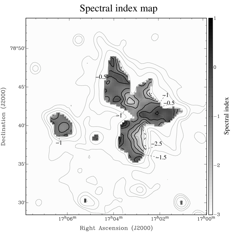
Figure 9: Spectral index map of Abell~2256 between 338 MHz and 365 MHz. The Stokes $I$ contours are drawn at 5, 10, 20, 40, 80, 160, 320 $\sigma$ of the 338 MHz map. The spectral index contours are drawn at $-3$–$+1$ in steps of 0.5. The accuracy is $0.46$ at the 40 sigma contour and $0.23$ at the 80 sigma contour.

In the simplest scenario, the energy spectral index $\gamma$ and total power of the injected electrons is constant. In this case, the radio spectrum consists of a power law with spectral index $\alpha_{\mathrm{low}}=-(\gamma-1)/2$ below the break frequency and a power law with spectral index $\alpha_{\mathrm{high}}=-\gamma/2$ above the break frequency. The half life time of synchrotron emitting electrons emitting in a magnetic field with strength $B$ in $\mu$G is

$$\tau=\frac{2.6\cdot 10^{10}\ \mathrm{years}}{B^{2}+B^{2}_{\mathrm{IC}}}\sqrt{\frac{B}{(1+z)\nu_{\mathrm{b}}}},$$ (10)

where $\nu_{\mathrm{b}}$ is the break frequency in MHz and $B_{\mathrm{IC}}$ is the strength of a magnetic field with the same energy density as the CMB. Assuming a CMB temperature of 2.725 K, its value is $3.238(1+z)^{2}\ \mu$G. The power laws fitted to the data in Fig. 8 intersect at $400\pm 180$ MHz. Substituting this value for the break frequency and the minimum energy magnetic fields determined above yields an age of $51_{-9}^{+18}$ million years if $B=7.3$ $\mu$G and $77_{-11}^{+27}$ million years if $B=4.8$ $\mu$G.

The above model is somewhat problematic because it implies that $\gamma\approx 3.4$, whereas in most head-tail sources $\gamma\approx 2.4$. It can therefore not be excluded that there is an additional break in the spectrum below $151$ MHz, where the spectral index flattens to $\alpha\approx-0.7$. This situation can occur when the power of the injection of relativistic plasma has decreased sharply after a period in which it was high and steady. The resulting spectrum has a spectral index of $-0.7$ below the hypothetical break at $\nu<151$ MHz and a spectral index of $-1.2$ above this break, followed by an exponential decrease. This increases the age estimates to $>83$ million years if $B=7.3$ $\mu$G and $>125$ million years $B=4.8$ $\mu$G. New observations below 150 MHz are needed in order to establish whether there is indeed an additional break in the spectrum. It is interesting to estimate the frequency range in which this break could occur.

Let us for the moment assume that F2 is indeed part of the tail of Fabricant galaxy 122. The galaxy is located at a distance of $2\aas@@fstack{\prime}6$ (180 kpc) from F2 in the plane of the sky. If F2 is indeed a section of the tail seen on-axis, one would expect that the galaxy travelled at least this far along the line of sight. The galaxy must therefore have travelled at least 0.25 Mpc. The current line-of-sight velocity of the galaxy is approximately 500 km s^-1 (Berrington et al. 2002). However, it is possible that the galaxy changed direction between F2 and F3 and is currently travelling approximately in the plane of the sky. Assuming that the actual velocity is of the order of the velocity dispersion of the cluster of approximately $1300$ km s^-1 (Berrington et al. 2002), the elapsed time since starting the electron injection into source F2 is at least 200 million years. A magnetic field of the order of $7.3$ $\mu$G then gives a break frequency of 26 MHz. This frequency will decrease if the source is older than 200 million years, but will increase if the magnetic field is lower than $7.3$ $\mu$G. Observations between 151 MHz and 10 MHz will be possible with LOFAR in the very near future, but will be very difficult below 20 MHz. A complete spectrum from 10 MHz to 5 GHz will enable a more accurate minimum energy magnetic field estimate by properly integrating the cosmic ray energies over the observed spectrum, instead of using a single power law. Until a better constrained synchrotron age for this source is obtained, its association with galaxy 122 remains uncertain.

4.4 Relic area

Relic without compact sources

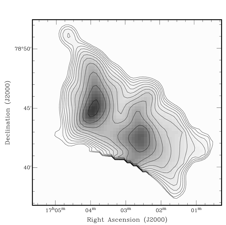
Figure 10: The relic area after subtraction of the halo and the tail of source C. The lowest contour is drawn at $1.5$ mJy beam^-1 and all subsequent contours are scaled by $\sqrt{2}$. The resolution is $67\arcsec$ FWHM.

The northwestern area of the cluster, dominated by the filaments G, H, and source C is perhaps the most intriguing part of Abell 2256. Most structure in that part is blended by the low resolution of Fig. 2, but Fig. 3 shows considerable detail.

At the resolution of Fig. 3, the long, straight tail of source C is striking. It is 11$\aas@@fstack{\prime}$5 (780 kpc) long at 351 MHz, which is considerably longer than the 7$\aas@@fstack{\prime}$08 (480 kpc) at 1446 MHz (Röttgering et al. 1994). At approximately $6\arcmin$ from the host galaxy, the tail begins to bend: first towards the northwest, then just after source I to the west-southwest and finally back to the northwest near source S. The period of the tentative oscillation is approximately 6′ (400 kpc) and the amplitude is about 0$\aas@@fstack{\prime}$6 (40 kpc).

Although it is not as detailed as the 1369 MHz VLA C configuration image of Clarke & Enßlin (2006), Fig. 3 clearly shows the filamentary nature of this part of the cluster. The FWHM of the brighter parts of filaments G and H is of the order of of 60″$\pm$15″ or 70$\pm$18 kpc. Filament G is approximately 10′ (680 kpc) long and filament H is approximately 8′ (550 kpc) from the tail of source C to the border of the relic emission directly south of source AC. There is a long, straight ridge south of the straight part of the tail of source C, at a position angle of approximately $210\degr$ (N through E). In fact this source may extend north of the tail of C into the southern part of filament H. If that is indeed the case, the source is $8\aas@@fstack{\prime}8$ (600 kpc) long. It appears to be unresolved at $26\arcsec$, limiting its width to less than 35 kpc.

The flux of the relic area was determined after subtracting Fig. 4 from Fig. 2. Sources A, B, and C were excluded. The extended tail of source C was removed by interpolating fluxes of pixels north and south of the tail using radial basis function interpolation (Carr et al. 2001). The resulting map is shown in Fig. 10. After correcting for the fact that the interpolated halo brightness in the relic area in Fig. 4 appears to be on average $1.5\pm 0.5$ mJy beam^-1 too high, the total flux in the relic area is $1.39\pm 0.07$ Jy. This is approximately a factor of three larger than the sum of the fluxes of the filaments G and H as determined by Röttgering et al. (1994). This discrepancy can be explained by the difference in uv coverage between the WSRT at 351 MHz and the VLA in B configuration at 327 MHz, which is not sensitive to scales above $7\arcmin$. The uv-coverage of the VLA-D observation by Clarke & Enßlin (2006) at 1369 MHz is much more similar to the WSRT at 351 MHz. Using their estimate of the relic flux, the spectral index between 1369 MHz and 351 MHz is $-0.81\pm 0.05$. This is much steeper than the 1446/327 MHz spectral index by Röttgering et al. (1994), but slightly flatter than the average 1703/1369 MHz spectral index that Clarke & Enßlin (2006) found.

Table 3: Rotation measures and linearly polarized fluxes of discrete sources within 1$\aas@@fstack{\circ}$5 of the optical centre of Abell 2256.

Nr.	Position		$\phi$	$|P_{\mathrm{a}}|$	$|P_{\mathrm{i}}|$
	(J2000 $\alpha$)	(J2000 $\delta$)	(rad m-2)	(mJy beam-1)	(mJy beam-1)
1	$16^{\mathrm{h}}47^{\mathrm{m}}02\aas@@fstack{s}7$	$+79\degr 06\arcmin 16\arcsec$	$-27.0\pm 0.1$	10.1	15.0
2	$16^{\mathrm{h}}49^{\mathrm{m}}07\aas@@fstack{s}7$	$+78\degr 51\arcmin 02\arcsec$	$-28.0\pm 0.8$	1.4	1.8
3	$16^{\mathrm{h}}51^{\mathrm{m}}45\aas@@fstack{s}1$	$+78\degr 09\arcmin 33\arcsec$	$-29.9\pm 0.8$	1.2	1.7
4	$17^{\mathrm{h}}00^{\mathrm{m}}30\aas@@fstack{s}7$	$+79\degr 30\arcmin 47\arcsec$	$-20.8\pm 0.2$	5.5	7.7
5	$17^{\mathrm{h}}00^{\mathrm{m}}53\aas@@fstack{s}6$	$+79\degr 30\arcmin 32\arcsec$	$-22.1\pm 0.2$	6.1	8.4
6	$17^{\mathrm{h}}05^{\mathrm{m}}18\aas@@fstack{s}4$	$+77\degr 47\arcmin 21\arcsec$	$-24.7\pm 0.5$	2.0	3.2
7	$17^{\mathrm{h}}05^{\mathrm{m}}55\aas@@fstack{s}5$	$+77\degr 06\arcmin 30\arcsec$	$-18.9\pm 0.2$	6.5	26.0
8	$17^{\mathrm{h}}06^{\mathrm{m}}14\aas@@fstack{s}4$	$+77\degr 07\arcmin 47\arcsec$	$-17.9\pm 0.2$	7.1	29.4
9	$17^{\mathrm{h}}07^{\mathrm{m}}17\aas@@fstack{s}0$	$+78\degr 06\arcmin 31\arcsec$	$-30.7\pm 0.5$	2.0	2.5
10	$17^{\mathrm{h}}18^{\mathrm{m}}44\aas@@fstack{s}7$	$+78\degr 39\arcmin 30\arcsec$	$-49.1\pm 0.3$	3.2	4.2
11	$17^{\mathrm{h}}23^{\mathrm{m}}34\aas@@fstack{s}7$	$+78\degr 29\arcmin 18\arcsec$	$-49.8\pm 0.5$	2.0	3.4

The spectral index map in Fig. 9 shows that the 365/338 MHz spectral index is far from uniform across the relic area. The average spectral index of filament H is $-1.17\pm 0.03$, which is comparable to its 1703/1369 MHz spectral index. The standard deviation of the spectral index distribution of filament H is 0.34.

The spectral index of the brightest part of filament G is $-0.70\pm 0.1$. Slightly north of that point is an east-west ridge with a 365/338 MHz spectral index of $-0.3$ to $-0.4$. There are several small areas with both steeper and flatter spectra. The average spectral index of filament G is $-0.76\pm 0.03$, which is significantly flatter than its 1703/1369 MHz spectral index Clarke & Enßlin (2006). The standard deviation of the spectral index distribution is 0.37.

5 Linear polarization

Galactic Faraday rotation

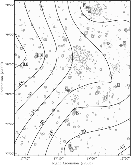
Figure 11: The Galactic Faraday rotation in rad m^-2 overlaid on Stokes $I$ contours. The Galactic RM is drawn at intervals of $5$ rad m^-2 and the total intensity contours at $-3$, 3, 12, 48, 192 $\times$0.6 mJy beam^-1. The polarized sources from Table 3 are indicated with crosses.

Although the relic area is between 20% and 50% polarized at 1.4 GHz (Clarke & Enßlin 2006; Bridle et al. 1979), there was no linearly polarized emission at 351 MHz at rotation measures between $-800$ and $+800$ rad m^-2 that could be attributed to the cluster. The relic area must therefore be substantially depolarized. This is not surprising, as already noted by Jägers (1987) at 610 MHz. A search in the area around Abell~2256 for structures similar to those attributed to the Perseus cluster (de Bruyn & Brentjens 2005) or found near Abell~2255 by Govoni et al. (2005) did not uncover anything. The only visible polarized sources were the Galactic synchrotron foreground at $\phi$ between $-20$ and $-24$ rad m^-2 and the collection of nine discrete sources (two doubles) listed in Table 3.

These sources made it possible to estimate the Galactic contribution to the Faraday depth of the relic much more accurately than the current estimate of $-4\pm 37$ rad m^-2 (Clarke & Enßlin 2006). A coarse estimate is obtained by taking the mean value of the Faraday depths of the sources, which results in $-29\pm 3$ rad m^-2.

A better approach is to interpolate the Faraday depths of the sources. The result is displayed in Fig. 11. The Galactic Faraday depth field was estimated using a radial basis function interpolation (Carr et al. 2001). The interpolated Galactic foreground contribution in the direction of the relic is $-33\pm 2$ rad m^-2. Subtracting this from the average RM of the relic that Clarke & Enßlin (2006) found ($-44$ rad m^-2), yields a cluster contribution of $-11\pm 2$ rad m^-2.

Using an isothermal beta model determined by Mohr et al. (1999) from ROSAT PSPC data (see Eq. (11)) and assuming that magnetic fields are frozen in (see Eq. (12)), this corresponds to a large scale magnetic field strength at the centre of the cluster of at least 0.08 $\mu$G if the relic were situated at the same distance as the cluster centre, and at least 0.4 $\mu$G if the relic is 500 kpc closer to the earth.

The depolarization of the relic emission gives a handle on the conditions inside the filaments. Because there is no significant polarized flux in the relic area at 351 MHz, only upper limits to the polarization fraction can be established. Figure 12 shows a map of the upper limits to the polarization fraction at 351 MHz. The maximum value of $|F(\phi)|$ for $-800\leq\phi\leq+800$ rad m^-2 was determined for each pixel. Refer to (Burn 1966; Gardner & Whiteoak 1966; Sokoloff et al. 1998; Brentjens & de Bruyn 2005) for definitions of the Faraday dispersion function $F(\phi)$. This map was then divided by the map in Fig. 2. The resulting upper limits are approximately a factor of four higher than upper limits obtained by dividing the image of the RMS value of $|F(\phi)|$ in the same range of $\phi$ by Fig. 2. Because $\mbox{RMS}=\sigma\sqrt{2}$ if the noise distribution is Gaussian, this corresponds approximately to a 6$\sigma$ upper limit.

The fractional polarization is less than 1% in the brightest parts of filaments G and H at 351 MHz. The maps by Jägers (1987) give a $3\sigma$ upper limit of 20% at these locations at 608.5 MHz. Clarke & Enßlin (2006) find about 28% polarization at both locations at 1369 MHz, with a resolution of $52\arcsec\times 45\arcsec$. They furthermore find, without precisely specifying how it is spatially distributed, that the polarization fraction at 1703 MHz is generally about 8% higher than at 1369 MHz, which would imply roughly 30% polarization at these locations.

Given the high degree of polarization at a resolution of the order of an arcminute at 1.4 GHz, the small spatial variance in RM, and the smooth structure in polarization angle that Clarke & Enßlin (2006) find, it is unlikely that the sharp decrease in polarization fraction with increasing wavelength is due to beam depolarization. The narrow channels, combined with RM-synthesis, rule out bandwidth depolarization at $|\phi|\lesssim 800$ rad m^-2. This leaves differential Faraday rotation along the line of sight, caused by the co-location of emitting plasma and Faraday rotating plasma as the most likely cause of the depolarization. The depolarization can be used to determine the Faraday thickness, or the extent in Faraday depth, of the radio emitting plasma.

351 MHz fractional polarization limits

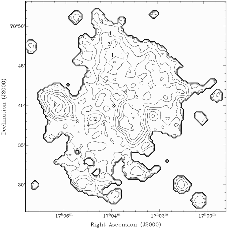
Figure 12: Upper limits ($\approx 6\sigma$, refer to the text for details) to the polarization fraction in percent at 351 MHz at a resolution of 67″ FWHM. Contours are drawn at 0.5%, 1%, 2%, 4%, 8%, 16%.

The depolarization data are plotted in Fig. 13. Although an accurate determination of the Faraday thickness requires new, sensitive polarization observations between 0.4 and 1.4 GHz, it is interesting to obtain an estimate of the extent of the relic sources in Faraday depth using the available detections and limits.

The uniform polarization angle structure at 1.4 GHz indicates that the magnetic field is relatively regular, perhaps even uniform at scales of a few arcminutes. If the relic has a uniform electron density, its structure in Faraday depth can be approximated by a uniform slab model (Burn 1966). The fractional polarization as a function of $\lambda^{2}$ of a uniform slab is a sinc function. The sinc curve in Fig. 13 corresponds to a slab with a full width of 21 rad m^-2 in Faraday depth. As can be seen in Fig. 13, it is impossible for a sinc function to simultaneously satisfy the Clarke & Enßlin (2006) points as well as the upper limits presented in this paper. The uniform slab model is therefore rejected. The Gaussian that is plotted in Fig. 13 has a FWHM of 4.7 rad m^-2 in Faraday depth and satisfies all upper limits and the two points by Clarke & Enßlin (2006). A Gaussian was chosen because it is a function that smoothly goes from a high value to a low value and has an easy analytical Fourier transform. Because this particular Gaussian satisfies all points rather closely without exceeding the limits, the FWHM of 4.7 rad m^-2 is considered a lower limit to the extent of filament G in Faraday depth. A more physical model will nevertheless have to wait until more sensitive observations between 400 MHz and 1.4 GHz are available.

6 Magnetic field in filament G

Depolarization of filament G

Figure 13: Polarization fraction of the brightest part of filament G as a function of wavelength squared. The point by Jägers (1987) is a 3$\sigma$ upper limit. The point at the bottom right is half the limit from Fig. 12 and is therefore equivalent to a 3$\sigma$ upper limit. The horizontal bars indicate the $\lambda^{2}$ coverage of the observations.

It is possible, with appropriate assumptions, to derive the magnetic field strength in filament G from its depolarization properties as displayed in Fig. 13.

According to the isothermal beta model (Cavaliere & Fusco-Femiano 1976) determined by Mohr et al. (1999) from ROSAT PSPC data,

$$\frac{n_{\mathrm{e}}(b,l)}{n_{\mathrm{e,0}}}=\left(1+\frac{b^{2}+l^{2}}{r_{\mathrm{c}}^{2}}\right)^{-3\beta/2},$$ (11)

where $n_{\mathrm{e}}(b,l)$ is the thermal electron density at impact parameter $b$ and line of sight distance between the cluster centre and the position $l$ (see Fig. 14), $n_{\mathrm{e,0}}=3.60\pm 0.06\times 10^{-3}h_{71}^{\frac{1}{2}}$ cm^-3 is the central electron density, $r_{\mathrm{c}}=342\pm 30h_{71}^{-1}$ kpc is the core radius, and $\beta=0.828\pm 0.06$ is the ratio of the specific kinetic energies of galaxies and gas. The impact parameter of the brightest part of filament G with respect to the centre of the X-ray source is 6$\aas@@fstack{\prime}$9 (470$\pm 15$ kpc). Clarke & Enßlin (2006) established that the relic must be on the front side of the cluster due to the small variance of the observed RMs. In the remainder of this section it is assumed that the brightest point of filament G lies approximately 500 kpc in front of the centre of the cluster ($l\approx-500$ kpc). The expected thermal electron density in the neighbourhood of the filament is then approximately $4.8\times 10^{-4}$ cm^-3.

Following the reasoning of Murgia et al. (2004), the magnetic field strength is assumed to be a power law of the thermal electron density:

$$\|\@vec{B}\|=an_{\mathrm{e,th}}^{\mu/\beta},$$ (12)

where $a$ is the proportionality constant. If the magnetic energy density is proportional to the gas energy density, $\mu=\beta/2$. If the magnetic field is frozen in the plasma, then $\mu=2\beta/3$. I only consider the latter case because the difference between the two is barely noticeable in view of the uncertainties involved.

Sketch of the cluster

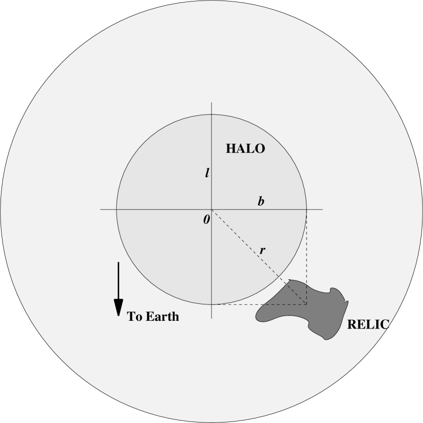
Figure 14: Coordinate system used for the computations in Sect. 6.

The relativistic electrons in relic sources such as filaments G and H are assumed to be shock accelerated (Enßlin et al. 1998). Merger shocks and accretion shocks typically compress the gas by a factor of up to 4 (Blandford & Ostriker 1978). For the sake of simplicity it was assumed that the resulting thermal electron density as a function of position along the line of sight has an offset Gaussian shape:

$$n_{\mathrm{e,th}}(\@vec{l}-\@vec{l_{0}})=n_{\mathrm{e,0}}\left(1+\left(r-1\right)\mathrm{e}^{-4\log{2}\left(\frac{\@vec{l}-\@vec{l_{0}}}{w}\right)^{2}}\right),$$ (13)

where $r$ is the shock compression ratio, $w$ is the FWHM of the compressed area, and $n_{\mathrm{e,0}}=4.8\times 10^{-4}$ cm^-3 is the expected electron density near the relic as calculated using Eq. (11).

The synchrotron radiation is caused by relativistic electrons, which have a much lower density. The synchrotron intensity from a slice of plasma with infinitesimal thickness $\mathrm{d}x$ is (see e.g. Pfrommer et al. 2008)

$$I(l)\ \mathrm{d}l\propto\frac{n_{\mathrm{e,rel}}\|\@vec{B}\|^{1-\alpha}}{\|\@vec{B}\|^{2}+B_{\mathrm{IC}}^{2}}\ \mathrm{d}l,$$ (14)

where $B_{\mathrm{IC}}=3.238(1+z)^{2}\ \mu$G is the contribution from inverse Compton losses due to cosmic microwave background photons and $\|\@vec{B}\|$ is given by Eq. (12).

It is assumed that there are only significant amounts of relativistic electrons in the compressed area. More specifically, the relativistic electron density is assumed to be a Gaussian with unit peak and the same FWHM $w$ as the compression peak in the thermal electron distribution. The absolute number of relativistic electrons is unimportant for depolarization arguments. Only the shape of the distribution matters. Figure 15 shows an example of a thermal electron density profile with its accompanying relativistic electron density profile. Note that the vertical scale of the relativistic profile is arbitrary. More precise modelling is not useful at this point because there are only upper limits available below 1369 MHz.

The Faraday depth $\phi(l)$ of a given location is obtained by integrating

$$\frac{\mathrm{d}\phi}{\mathrm{d}l}=0.81a\times n_{\mathrm{e,th}}^{\frac{5}{3}}$$ (15)

from $l=-2w$ to the location of interest. The Faraday dispersion function

$$F(\phi)=I(\phi)/\frac{\mathrm{d}\phi}{\mathrm{d}l}.$$ (16)

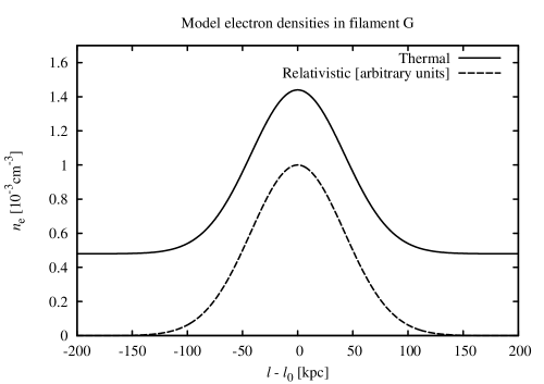
Figure 15: Model electron densities used for estimating the magnetic field in filament G. The model densities are plotted as a function of position along the line of sight with respect to the centre of filament G. The FWHM of the peaks is 100 kpc. The vertical scale applies to the thermal electron density only. The peak gas compression ratio in this plot is three.

From symmetry arguments one expects the FWHM thickness of the emitting filaments in the relic to be of the order of 30–100 kpc. Figure 16 shows the peak magnetic field in the relic as a function of the shock compression ratio for FWHM thicknesses from 25 to 400 kpc. The peak field strength was derived by finding the value of $a$ that created a FWHM of $F(\phi)$ of either 21 or 4.7 rad m^-2, which was subsequently substituted into Eq. (12).

As Fig. 16 shows, the field estimate depends on the assumptions about the shock compression ratio and the extent of the filament in both geometric space as well as Faraday space. A value of the order of $0.2$ $\mu$G appears reasonable assuming a relic thickness of the order of 30 kpc and an extent in Faraday depth of 4.7 rad m^-2 FWHM. However, due to the uncertainties involved this value may be off by a factor of up to 10.

7 Conclusions and future work

The spectral index of the diffuse central halo of Abell~2256 is $-1.61\pm 0.04$. Although this value is steeper than the 610/1415 MHz value of $-1.2$ in Bridle et al. (1979), it is somewhat flatter than their 150/610 MHz spectral index ($-1.8$) and considerably flatter than the value of $-2.04$ derived by Kim (1999). The reason for this is twofold:

• in Clarke & Enßlin (2006) and in this work, the halo was detected over a larger extent than in previous observations by Bridle et al. (1979) and Kim (1999) due to the increased sensitivity of the observations;

• Kim (1999) did not correct the 81.5 MHz flux (Branson 1967) as proposed by Masson & Mayer (1978).

The observed spectral index puts the classical minimum energy magnetic field in the range of 2–4 $\mu$G, and the hadronic minimum energy field between 4 and 9 $\mu$G (Clarke & Enßlin 2006).

Despite the deep polarization images obtained after RM-synthesis, no polarized emission was detected that could be attributed to Abell 2256. The complete depolarization of filaments G and H was expected because of the relatively high density environment in which they reside. The upper limit to the fractional polarization of less than 1% is consistent with the 608.5 MHz upper limit by Jägers (1987) and the depolarization between 1705 MHz and 1395 MHz that Clarke & Enßlin (2006) found.

Figure 16: Estimates of the magnetic field parallel to the line of sight in filament G.

Reliable measurements of the magnetic field in relic sources are relatively rare. Bagchi et al. (1998) used inverse Compton scattering to derive the cluster scale magnetic field in the relic of Abell~85. They found a value of $0.95\pm 0.10$ $\mu$G. Chen et al. (2008) derived classical equipartition field strengths of 0.63 and 1.3 $\mu$G for the relics in 0917+75 and 1401-33 respectively. Their $3\sigma$ inverse Compton lower limits are 0.81 and 2.2 $\mu$G. Enßlin et al. (1998) listed an equipartition field of $3h_{71}^{2/7}$ $\mu$G for the entire relic in Abell 2256. Although the estimate of the line-of-sight field in filament G presented in this work is not very accurate ($0.02$–$2$ $\mu$G with $0.2$ $\mu$G in case of reasonable assumptions about the shock compression ratio and path length along the line of sight), it is consistent with the quoted literature values for magnetic fields in relic sources in general. An actual measurement of the depolarization of filament G can improve the estimate significantly, although the major uncertainty is in the physical thickness of the relic along the line of sight, which is very difficult to obtain.

Polarization observations covering frequencies between 1.4 GHz and 400 MHz, where the fractional polarization decreases rapidly, would make it possible to recover the (linearly polarized) emissivity of filaments G and H as a function of Faraday depth along the line of sight. The high fractional polarization at 1.4 GHz ensures that the magnetic field has no reversals along the line of sight. Therefore, the Faraday depth of a certain location in the relic sources should be a monotonic function of the geometric distance between the front of the sources and that location, enabling the first 3D reconstruction of an extragalactic synchrotron source.

The fact that no evidence was found for polarized emission from LSS shocks or buoyant bubbles further away from the cluster centre than filaments G and H could have several reasons:

• they are depolarized due to internal Faraday dispersion, just like sources G and H;

• there are no shocks oriented edge-on, only face-on, resulting in an undetectably low surface brightness;

• apart from the relic area, there are simply no other bubbles or large scale shocks in Abell 2256 that emit radio waves.

The first point can be tested by applying RM-synthesis to deep polarimetry at 1.4 GHz. Discriminating between the other two possibilities would be difficult at best in a single cluster. One way to move forward is by observing a larger sample of nearby clusters at high Galactic latitude using RM-synthesis around 350 MHz. A fractional bandwidth of 20% is then sufficient to separate cluster emission from Galactic foreground emission. If RM-synthesis does not reveal any bubble-like polarized structures, similar to the ones towards the Perseus-cluster (de Bruyn & Brentjens 2005), it must be concluded that the structures detected towards the Perseus cluster really belong to the Galactic ISM. At this moment, however, there is not enough evidence to draw a final conclusion.