Solution of the Percus-Yevick equation for hard hyperspheres in even dimensions

Abstract

We solve the Percus-Yevick equation in even dimensions by reducing it to a set of simple integro-differential equations. This work generalizes an approach we developed previously for hard discs. We numerically obtain both the pair correlation function and the virial coefficients for a fluid of hyper-spheres in dimensions $d=4,6$ and $8$, and find good agreement with available exact results and Monte-Carlo simulations. This paper confirms the alternating character of the virial series for $d\geq 6$, and provides the first evidence for an alternating character for $d=4$. Moreover, we show that this sign alternation is due to the existence of a branch point on the negative real axis. It is this branch point that determines the radius of convergence of the virial series, whose value we determine explicitly for $d=4,6,8$. Our results complement, and are consistent with, a recent study in odd dimensions [R.D. Rohrmann et al., J. Chem. Phys. 129, 014510 (2008)].

I Introduction

In recent years, there has been much interest in the properties of hard sphere fluids. The study of such systems has played a central role in the understanding of classical fluids and serves as a starting point for the construction of perturbation theories of fluid properties. A particular interest has been systems of hard hyperspheres whitlock ; Skoge06 ; Lue05 ; Lue06 ; clisby06 ; B4 ; B3 ; clisby04b ; clisby05 ; Rohrmann ; rohrmann08 ; robles ; frisch (i.e. the generalization of spheres to dimensions larger than three, $d>3$). There are several reasons for this interest. Firstly, as in a variety of interacting many-body systems CL , one expects studies of hard-sphere packings in high dimensions to yield great insight into the corresponding phenomena in lower dimensions, such as ground and glassy states of matter Torquato02 ; Torquato06 . Secondly, it is hopedfrisch that analytical investigations of hard hyperspheres in large spatial dimensions can serve as an organizing device for a systematic expansion in inverse powers of the dimension, $d$. From a completely different perspective, hard hypersphere systems play an important role in communication theory. For example, it is known that the optimal way of sending digital signals over noisy channels correspond to the densest sphere packing in a high-dimensional space CS , so called “spherical codes”.

It is common to describe hard-core fluids using approximate theorieshansen . There are two main reasons for using such approximate theories: on the one hand, a solution of the full problem was, and still is, extremely difficult. On the other hand, approximate methods have led to very good predictions in the low density phase. Among the most widely used approximations is the Percus-Yevick (PY) equation for $d$-dimensional hard spheres PY , which is exact to first order in the density of the fluidrohrmann08 , $\rho$.

A great deal of progress has been made towards understanding the solutions of the PY equation in odd dimensions. In principle, the work of Baxterbaxter and Leutheusserleuth1 reduces the PY equation to a set of nonlinear algebraic equations of order $2^{(d-3)/2}$ for $d>3$. However, these can only be solved analytically for $d\leq 7$ so that results in higher odd dimensions must be found numerically. A more complete survey of the literature for odd dimensions may be found elsewhererohrmann08 .

In even dimensions the situation is much less developed. In two dimensions an approximate numerical solution of the PY equation was found by Lado lado . Leutheusser leuth2 was able to fit many of Lado’s results using an ansatz for the direct correlation function. Other results available in the literature for hard discs are solutions of the full problem based on Molecular Dynamics (MD) or Monte Carlo (MC) methods hoover67 ; numerics ; alder68 ; wood ; clisby06 . Recently, the authors solved the PY equation for hard discs PY2d , by developing a method that reduces the problem to a set of integral equations that are solved numerically without major difficulties.

In larger even dimensions there are some MD simulationsLue05 ; Lue06 ; Skoge06 , MC simulationswhitlock , MC calculations clisby04b ; clisby05 ; clisby06 and a few analytical results for the low order virial coefficients B3 ; B4 . On the analytical front, Rosenfeld rosenfeld generalized Leutheusser’s Ansatzleuth2 to higher dimensions and compared the results with the analytical results in three and five dimensions. However, to our knowledge, the PY equation has not been solved in any even dimension apart from $d=2$.

In this paper, we solve the PY equation for some even dimensions ($d=4,6$ and $8$). We do so by generalizing our previous work PY2d , which was based on techniques borrowed from the resolution of crack problems sned and uses some results from Baxter’s classical method hansen ; baxter . The main difference from the hard sphere case (and any odd dimension in general) is that the problem of finding the total correlation function and the direct correlation function are coupled. This means that the present analysis necessarily yields both correlation functions and therefore provides the equation of state. The advantage of the current method over previous approaches is that it provides all the quantities of interest as power-series in the density. Thus, questions like existence of negative virial coefficients in four dimensionsclisby04b and more generally the radius of convergence of the series in large dimensions rohrmann08 can be tackled.

II The Percus-Yevick approximation

The pair correlation function $g({\mathbf{r}})$ is related to the direct correlation function $c({\mathbf{r}})$ through the Ornstein-Zernike equation by hansen ; OZ

$$h({\mathbf{r}})=c({\mathbf{r}})+\rho\int_{0}^{\infty}h({\mathbf{r}^{\prime}})c(|\mathbf{r}-\mathbf{r^{\prime}}|)dr^{\prime}\,,$$ (1)

where $\rho$ is the particle number density and

$$h({\mathbf{r}})=g({\mathbf{r}})-1\,,$$ (2)

is the total correlation functionhansen . The PY approximation is a closure relation for Eq. (1). For a hard-core pair interaction potential, this approximation reads hansen

$$g(r) = h(r)+1=0,\qquad r<1$$ (3)

$$c(r) = 0,\qquad r>1$$ (4)

Interestingly, the PY approximation can be seen as a Random Phase Approximation (RPA) to some nonlinear field theory as shown previously SE .

Here and elsewhere, we take the diameter of the hypersphere to be unity. Thus in $d$ dimensions ($d=2(k+1)$, with $k\geq 0$), we have

$$\rho=\frac{\eta}{V_{d}(1/2)}=\left(\frac{4}{\pi}\right)^{k+1}(k+1)!\,\eta\,\,,$$ (5)

where

$$V_{d}(R)=\frac{\pi^{\frac{d}{2}}R^{d}}{\Gamma\left(\frac{d+2}{2}\right)},$$ (6)

is the volume of a $d$-dimensional hypersphere of radius $R$, $\eta$ is the packing fraction, and the space filling density corresponds to $\eta=1$. We define the $d$-dimensional Fourier Transform

$$\tilde{f}(q)=(2\pi)^{k+1}q^{-k}\int_{0}^{\infty}r^{k+1}J_{k}(qr)f(r)dr\,,$$ (7)

where $J_{k}$ is the Bessel function and the inverse Fourier transform for $f(r)$ and $F_{k}(r)$ are given by

$$f(r)=(2\pi)^{-(k+1)}r^{-k}\int_{0}^{\infty}q^{k+1}J_{k}(qr)\tilde{f}(q)dq\,,$$ (8)

Applying the $d$-dimensional Fourier transform to Eq. (1) yields

$$\tilde{h}(q)=\tilde{c}(q)+\rho\tilde{h}(q)\tilde{c}(q)\,,$$ (9)

which can be rewritten as

$$\left[1-\rho\tilde{c}(q)\right]\left[1+\rho\tilde{h}(q)\right]=1\,.$$ (10)

Finally, the static structure factor $s(q)$ of wavenumber ${\mathbf{q}}$ is related to the pair correlation function through

$$s(q)=1+\rho\tilde{h}(q)\equiv\frac{1}{1-\rho\tilde{c}(q)}\,.$$ (11)

III Resolution

The condition (4) together with (8) imposes that $\tilde{c}(q)$ can be written without loss of generality as

$$\tilde{c}(q)=\left(\frac{2\pi}{q}\right)^{k+\frac{1}{2}}\int_{0}^{1}t^{k+\frac{3}{2}}J_{k+\frac{1}{2}}(qt)\phi(t)dt$$ (12)

where $\phi(t)$ is a real function. Substituting (12) into (8) and simplifying by using the integral 6.575-1 in grads , we find that $c(r)$ can be expressed as

$$c(r)=\int_{r}^{1}\frac{t\phi(t)}{\sqrt{t^{2}-r^{2}}}\frac{dt}{\pi}\,,\qquad 0\leq r<1\,.$$ (13)

Since $c(r)$ is discontinuous yet finite at $r=1$, one has

$$\phi(t)\sim\left(1-t^{2}\right)^{-1/2}\qquad\mbox{as}\qquad t\rightarrow 1^{-}$$ (14)

In the following, we use the formulation of Baxter for the odd dimensional case, with the important difference that instead of solving for $c(r)$ directly, we solve for $\phi(t)$, and obtain $c(r)$ using Eq. (13). We use the Wiener-Hopf method by defining

$$A(q)\equiv\frac{1}{s(q)}=1-\rho\left(\frac{2\pi}{q}\right)^{k+\frac{1}{2}}\int_{0}^{1}t^{k+\frac{3}{2}}J_{k+\frac{1}{2}}(qt)\phi(t)dt$$ (15)

One sees that $A(q)=A(-q)$, $A(q)\rightarrow 1$ as $q\rightarrow\infty$ and that $A(q)$ has the same properties as the corresponding function defined in the odd dimensional case: it has neither zeros nor poles on the real axis, since by definition $s(q)$ has neither zeros nor poles for all $q$’s. Therefore one can use the Wiener-Hopf decomposition of Baxter hansen ; baxter

$$A(q)=\tilde{Q}(q)\tilde{Q}(-q)$$ (16)

where $\tilde{Q}(q)$ is analytic for $\Im(q)>0$. Following the same steps as in hansen ; baxter ; PY2d one can show that $\tilde{Q}(q)$ can be written as

$$\tilde{Q}(q)=1-\lambda\int_{0}^{1}Q(t)e^{iqt}dt$$ (17)

where $\lambda$ is a parameter defined by

$$\lambda\equiv(2\pi)^{k}\rho$$ (18)

and thus using (15)-(17)

$$\rho \left(\frac{2\pi}{q}\right)^{k+\frac{1}{2}}\int_{0}^{1}s^{k+\frac{3}{2}}J_{k+\frac{1}{2}}(qs)\phi(s)ds$$ (19)

$$= \lambda\int_{0}^{1}Q(s)e^{iqs}ds+\lambda\int_{0}^{1}Q(s)e^{-iqs}ds$$

$$- \lambda^{2}\int_{0}^{1}ds\int_{0}^{1}ds^{\prime}Q(s)Q(s^{\prime})e^{iq(s-s^{\prime})}$$

Multiplying by $\exp(-iqt)$, with $0\leq t\leq 1$ and integrating with respect to $q$ from $-\infty$ to $\infty$ gives

$$\sqrt{\frac{2}{\pi}}\int_{0}^{1}ds\,s^{k+\frac{3}{2}}\phi(s)\int_{0}^{\infty}dq\,q^{-(k+\frac{1}{2})}J_{k+\frac{1}{2}}(qs)\cos qt$$

$$=Q(t)-\lambda\int_{t}^{1}Q(s)Q(s-t)ds$$ (20)

which can be simplified to give

$$\int_{t}^{1}(s^{2}-t^{2})^{k}\phi(s)sds=2^{k}k!\left[Q(t)-\lambda\int_{t}^{1}Q(s)Q(s-t)ds\right].$$ (21)

Differentiating $k$-times with respect to $t^{2}$ and once with respect to $t$ gives

$$\phi(t)=(-1)^{k+1}\left(\frac{d}{tdt}\right)^{k+1}\left[Q(t)-\lambda\int_{t}^{1}Q(s)Q(s-t)ds\right]\,,$$ (22)

which is valid for $0\leq t\leq 1$. Therefore, once $Q(t)$ is known, $\phi(t)$ is given by Eq. (22) and $c(r)$ is given by Eq. (13).

Now let us work on the function $h(r)$. Since $\tilde{h}(q)$ is an even function one can write without loss of generality

$$\tilde{h}(q)=\left(\frac{2\pi}{q}\right)^{k+\frac{1}{2}}\int_{0}^{\infty}t^{k+\frac{3}{2}}J_{k+\frac{1}{2}}(qt)\psi(t)dt$$ (23)

where $\psi(t)$ is a real function. Then, using Eq. (8) $h(r)$ can be written in terms of $\psi(t)$ as

$$h(r)=\int_{r}^{\infty}\frac{t\psi(t)}{\sqrt{t^{2}-r^{2}}}\frac{dt}{\pi}\,,\qquad r>0\,.$$ (24)

Combining this equation together with the condition (3), one obtains

$$\int_{r}^{1}\frac{t\psi(t)}{\sqrt{t^{2}-r^{2}}}\frac{dt}{\pi}=-1-\int_{1}^{\infty}\frac{t\psi(t)}{\sqrt{t^{2}-r^{2}}}\frac{dt}{\pi}\,,\qquad 0<r<1\,.$$ (25)

This is an integral equation of Abel type that we can invert. As shown in PY2d the inversion of the equation is given by

$$\psi(t)=\frac{-2}{\sqrt{1-t^{2}}}\left[1+\int_{1}^{\infty}\frac{\sqrt{s^{2}-1}}{s^{2}-t^{2}}s\psi(s)\frac{ds}{\pi}\right]\,,\qquad 0<t<1\,.$$ (26)

Eq. (26) is an integral equation that determines $\psi(t)$ for $0<t<1$ as function of $\psi(t)$ for $t>1$. Also, note that the behavior of $\psi(t)$ near $t=1$ is

$$\psi(t)\sim\left(1-t^{2}\right)^{-1/2}\qquad\mbox{as}\qquad t\rightarrow 1^{-}$$ (27)

Substituting the results of Eqs. (11), (15)-(17) and (23) into Eq. (10) gives

$$\frac{1}{\tilde{Q}(-q)} = \left[1-\lambda\int_{0}^{1}Q(s)e^{iqs}ds\right]$$

$$\times \left[1+\rho\left(\frac{2\pi}{q}\right)^{k+\frac{1}{2}}\int_{0}^{\infty}t^{k+\frac{3}{2}}J_{k+\frac{1}{2}}(qt)\psi(t)dt\right]$$

Multiplying by $\exp(-iqt)$ with $t>0$ and integrating with respect to $q$ from $-\infty$ to $\infty$ we obtain

$$2^{k}k!\int_{0}^{1}Q(s)\delta(s-t)ds-\int_{t}^{\infty}(s^{2}-t^{2})^{k}\psi(s)sds$$

$$+ \lambda\int_{0}^{1}dsQ(s)\int_{|t-s|}^{\infty}(s^{\prime 2}-(s-t)^{2})^{k}\psi(s^{\prime})s^{\prime}ds^{\prime}=0$$

which leads to

$$2^{k}k!Q(t)\Theta(1-t)-\int_{t}^{\infty}(s^{2}-t^{2})^{k}\psi(s)sds$$ (30)

$$=-\lambda\int_{0}^{1}dsQ(s)\int_{|t-s|}^{\infty}(s^{\prime 2}-(t-s)^{2})^{k}\psi(s^{\prime})s^{\prime}ds^{\prime}\,,$$

where $\Theta(x)$ is the Heaviside function. Recall that $\psi(t)$ is defined only for $t>0$. Therefore one has

$$2^{k}k!\,Q(t)-\int_{t}^{\infty}(s^{2}-t^{2})^{k}\psi(s)sds = -\lambda\int_{0}^{1}ds\,Q(s)\int_{|t-s|}^{\infty}(s^{\prime 2}-(t-s)^{2})^{k}\psi(s^{\prime})s^{\prime}ds^{\prime}\qquad 0<t<1$$ (31)

$$\int_{t}^{\infty}(s^{2}-t^{2})^{k}\psi(s)sds = \lambda\int_{0}^{1}ds\,Q(s)\int_{(t-s)}^{\infty}(s^{\prime 2}-(t-s)^{2})^{k}\psi(s^{\prime})s^{\prime}ds^{\prime}\qquad t>1$$ (32)

Replacing $\psi(t)$ for $0<t<1$ in Eq. (31) with its value as given by Eq. (26) yields an equation that depends only on $\psi(t)$ for $t>1$, namely

$$Q(t)=A(t)+\int_{1}^{\infty}B(s,t)\psi(s)sds-\lambda\int_{0}^{1}\left[A(t-s)+\int_{1}^{\infty}B(s^{\prime},t-s)\psi(s^{\prime})s^{\prime}ds^{\prime}\right]Q(s)ds\qquad 0<t<1$$ (33)

with

$$A(t) = -\frac{2}{(2k+1)!!}(1-t^{2})^{k+\frac{1}{2}}$$ (34)

$$B(s,t) = \frac{1}{2^{k}k!}(s^{2}-t^{2})^{k}\,I\left(\frac{s^{2}-1}{s^{2}-t^{2}};\frac{1}{2},\frac{1}{2}+k\right)$$ (35)

where $I(z;a,b)$ is the regularized Beta function abram . On the other hand, using Eq. (26) and differentiating $k$-times with respect to $t^{2}$ and once with respect to $t$ one can rewrite Eq. (32) as

$$\psi(t) = -(-1)^{k}\lambda\left(\frac{d}{tdt}\right)^{k+1}\int_{t-1}^{1}\left[A(t-s)+\int_{1}^{\infty}B(s^{\prime},t-s)\psi(s^{\prime})s^{\prime}ds^{\prime}\right]Q(s)ds$$ (36)

$$-(-1)^{k}\frac{\lambda}{2^{k}k!}\left(\frac{d}{tdt}\right)^{k+1}\int_{0}^{t-1}\left[\int_{(t-s)}^{\infty}(s^{\prime 2}-(t-s)^{2})^{k}\psi(s^{\prime})s^{\prime}ds^{\prime}\right]Q(s)ds\qquad 1<t<2$$

$$\psi(t) = -(-1)^{k}\frac{\lambda}{2^{k}k!}\left(\frac{d}{tdt}\right)^{k+1}\int_{0}^{1}\left[\int_{(t-s)}^{\infty}(s^{\prime 2}-(t-s)^{2})^{k}\psi(s^{\prime})s^{\prime}ds^{\prime}\right]Q(s)ds\qquad t>2$$ (37)

Our approach has reduced the PY problem for hard hyperspheres to the solution of the set of one-dimensional integro-differential equations (33),(36) and (37) for the auxiliary functions $\psi(s)$ and $Q(s)$. Once these functions have been determined, the physically relevant functions may be determined; $g(r)$ from (2) and (24), $c(r)$ from (13) and (22). We note that unlike the odd dimensional case leuth1 , in even dimensions it is not possible to separate the problem of finding the direct correlation function $c(r)$ from that of finding the pair correlation function $g(r)$. This is because the behavior of the auxiliary function $\psi(t)$ for $0<t<1$ is coupled to its behavior for $t>1$ through Eq. (26). Although we were unable to find an analytical solution valid for all $\rho$, a numerical algorithm to find the numerical solution of these equations can easily be implemented. Before dealing with the numerical analysis, let us first consider the equation of state in the present formulation of the problem.

IV Equation of state

There are two methods used to calculate the equation of state when the radial distribution function, $g(r)$, is known. Without the assumptions made in deriving the PY equation PY , these two methods would yield the same equation of state. The difference in the equations of state calculated using these two methods therefore provides an estimation of the error made by using the PY approximation. The first method of calculating the equation of state uses the isothermal compressibility $\kappa_{T}$ which is given by hansen

$$\rho\beta^{-1}\kappa_{T}=\frac{1}{\beta}\,\left(\frac{\partial\rho}{\partial P^{(c)}}\right)_{T}=s(q=0)\,,$$ (38)

where $\beta$ is the inverse temperature $1/k_{B}T$. Using Eqs. (15) and (12), it is easy to deduce that

$$\frac{1}{s(0)}=1-\frac{2(2\pi)^{k}\rho}{(2k+1)!!}\int_{0}^{1}t^{2(k+1)}\phi(t)dt\,,$$ (39)

which can be further simplified by successive integration by parts to give

$$\frac{1}{s(0)}=1-\frac{2\pi^{k}\rho}{k!}\int_{0}^{1}dt\left[\int_{t}^{1}(s^{2}-t^{2})^{k}\phi(s)sds\right]\,.$$ (40)

Using Eq. (21) we may eliminate $\phi(s)$ to yield

$$\frac{1}{s(0)}=1-2\lambda\int_{0}^{1}\left[Q(t)-\lambda\int_{t}^{1}Q(s)Q(s-t)ds\right]dt$$ (41)

Thus, the compressibility equation of state can be written as

$$\frac{\beta\,P^{(c)}}{\rho}-1=$$ (42)

$$-\frac{2}{\lambda}\int_{0}^{\lambda}\left\{\int_{0}^{1}\left[Q(t)-\lambda^{\prime}\int_{t}^{1}Q(s)Q(s-t)ds\right]dt\right\}\lambda^{\prime}d\lambda^{\prime}\,,$$

The second method to obtain the equation of state is derived from the virial theorem and is given by

$$\beta\,P^{(v)}=\rho+\frac{\pi^{k+1}}{(k+1)!}\,\frac{\rho^{2}}{2}\,g(1^{+})\,.$$ (43)

Finally, using Eqs. (2) and (24), Eq. (43) becomes

$$\frac{\beta P^{(v)}}{\rho}-1=\frac{\pi\lambda}{2^{k+1}(k+1)!}\left[1+\int_{1}^{\infty}\frac{s\psi(s)}{\sqrt{s^{2}-1}}\frac{ds}{\pi}\right]\,,$$ (44)

where $\lambda$ is defined in (18).

V Numerical Procedure

As in our earlier work PY2d , we solve Eqs. (33),(36) and (37) for the auxiliary functions $Q(s)$ and $\psi(s)$ iteratively. However, the present method of solution is simpler than the one used previously, as explained below. We pose power series

$$Q(t) = \sum_{i=0}^{\infty}\lambda^{i}q_{i}(t)\,,\qquad 0<t<1\,,$$ (45)

$$\psi(t) = \sum_{i=0}^{\infty}\lambda^{i}\psi_{i}(t)\,,\qquad t>1\,,$$ (46)

for the unknown functions, and substitute these power series into Eqs. (33),(36) and (37). At zeroth order, we obtain

$$q_{0}(t)=A(t);\quad\psi_{0}(t)=0\,.$$ (47)

For $i\geq 0$, we find

$$\psi_{i+1}(t) = -(-1)^{k}\left(\frac{d}{tdt}\right)^{k+1}\sum_{j=0}^{i}\int_{t-1}^{1}\left[A(t-s)\delta_{j,i}+\int_{1}^{\infty}B(s^{\prime},t-s)\psi_{i-j}(s^{\prime})s^{\prime}ds^{\prime}\right]q_{j}(s)ds$$ (48)

$$-\frac{(-1)^{k}}{2^{k}k!}\left(\frac{d}{tdt}\right)^{k+1}\sum_{j=0}^{i}\int_{0}^{t-1}\left[\int_{(t-s)}^{\infty}(s^{\prime 2}-(t-s)^{2})^{k}\psi_{i-j}(s^{\prime})s^{\prime}ds^{\prime}\right]q_{j}(s)ds,\qquad 1<t<2;$$

$$\psi_{i+1}(t) = -\frac{(-1)^{k}}{2^{k}k!}\left(\frac{d}{tdt}\right)^{k+1}\sum_{j=0}^{i}\int_{0}^{1}\left[\int_{(t-s)}^{\infty}(s^{\prime 2}-(t-s)^{2})^{k}\psi_{i-j}(s^{\prime})s^{\prime}ds^{\prime}\right]q_{j}(s)ds,\qquad t>2;$$ (49)

$$q_{i+1}(t) = \int_{1}^{\infty}B(s,t)\psi_{i+1}(s)sds-\sum_{j=0}^{i}\int_{0}^{1}\left[A(t-s)\delta_{j,i}+\int_{1}^{\infty}B(s^{\prime},t-s)\psi_{i-j}(s^{\prime})s^{\prime}ds^{\prime}\right]q_{j}(s)ds,\;0<t<1.$$ (50)

We use an iterative procedure, starting with (47), to calculate successively $\psi_{i}(t)$ and then $q_{i}(t)$ using (48)-(50). In the above formulation of the problem, the only difficulty is that one has to differentiate $(k+1)$-times. However, this is balanced by the fact that the integrals to be computed have no singular behavior, in contrast with our earlier method of solution for the case $k=0$ (i.e. $d=2$)PY2d .

Rather than computing the equation of state for various densities $\rho$ (as in earlier worklado ), we compute the virial coefficients, $B_{i}$, which are defined by

$$\beta\,P=\sum_{i=1}^{\infty}B_{i}\rho^{i}\,.$$ (51)

Thanks to the iterative procedure presented above, these coefficients, namely $B_{i}^{(c)}$, from the compressibility route (IV), and $B_{i}^{(v)}$, from the virial route (44), are directly given by the numerical resolution of the problem.

The first two coefficients are identical and may be computed analytically:

$$B_{1}^{(c)}=B_{1}^{(v)}=1\,,$$ (52)

and

$$B_{2}^{(c)}=B_{2}^{(v)}=\frac{\pi^{k+1}}{2(k+1)!}\,.$$ (53)

Higher order coefficients must be found numerically. For $i\geq 1$ we find

$$B_{i+2}^{(c)} = -\frac{2(2\pi)^{k(i+1)}}{i+2}$$

$$\times \int_{0}^{1}\left[q_{i}(t)-\sum_{j=0}^{i-1}\int_{t}^{1}q_{j}(s)q_{i-1-j}(s-t)ds\right]dt\,.$$

and

$$B_{i+2}^{(v)}=\frac{(2\pi)^{k(i+1)}}{2^{k+1}(k+1)!}\int_{1}^{\infty}\frac{s\psi_{i}(s)}{\sqrt{s^{2}-1}}ds\,,$$ (55)

The calculation of the first two virial coefficients via the two routes (c and v) produce identical results (coincident with the exact results) because the PY approximation is exact up to first order rohrmann08 in $\rho$. What is not so evident is that for the same reason both the third virial coefficient and the first order pair correlation function, $g_{1}(r)$, are also reproduced exactly by the PY theory. $B_{3}$ is given in closed form byB3

$$B_{3}^{(c)}=B_{3}^{(v)}=B_{3}^{exact}=\frac{\pi^{2k+2}}{2[(k+1)!]^{2}}\frac{B_{3/4}(k+\frac{3}{2},\frac{1}{2})}{B(k+\frac{3}{2},\frac{1}{2})}\,,$$ (56)

where $B(a,b)=\Gamma(a)\Gamma(b)/\Gamma(a+b)$ is the beta function, $B_{x}(a,b)$ is the incomplete beta function abram . Note that for each integer dimension this expression can be written in a simpler form without the need for transcendental functions. However, it is not possible to write a simpler general form. Furthermore, $g_{1}(r)$ is given by

$$g_{1}(r)=1+\int_{r}^{\infty}\frac{t\psi_{1}(t)}{\sqrt{t^{2}-r^{2}}}\frac{dt}{\pi}=\Theta(r-1)\left[1+2^{d}\alpha_{2}(r;1)\right]\,,$$ (57)

where $\alpha_{2}(r;1)$ is the scaled intersection volume Torquato02 ; Torquato06 .

It is also worthwhile mentioning that $B_{4}$ was recentlyB4 evaluated exactly for all dimensions up to $d=12$, though a closed-form formula for any $d$ is not available. We reproduce the values of $B_{4}$ for even dimensions $d\leq 8$, of interest here, in Table 1.

$d$	$B_{4}^{exact}$	$B_{4}^{Numercial}$
2	$\frac{\pi^{3}}{8}\left(2-\frac{9\sqrt{3}}{2\pi}+\frac{10}{\pi^{2}}\right)$	$2.062$
4	$\frac{\pi^{6}}{64}\left(2-\frac{27\sqrt{3}}{4\pi}+\frac{832}{45\pi^{2}}\right)$	$2.281$
6	$\frac{\pi^{9}}{1728}\left(2-\frac{81\sqrt{3}}{10\pi}+\frac{38848}{1575\pi^{2}}\right)$	$0.576$
8	$\frac{\pi^{12}}{110592}\left(2-\frac{2511\sqrt{3}}{280\pi}+\frac{17605024}{606375\pi^{2}}\right)$	$-0.021$

Table 1: The exact expressions for $B_{4}$ as well as their corresponding numerical values for some even dimensions obtained recently B4 .

We note that the computation of the correlation function $g(r)$ and the equation of state do not present any significant difficulties. The integrands that must be computed in the calculation of the coefficients $B_{i}^{(v)}$, see (55), and $g(r)$, see (24), have weak square root singularities that may be dealt with by integration by parts or by subtraction of the singularity. We validate our numerical implementation of the iterative procedure outlined above by comparing our results with the earlier results for the case $k=0$ (i.e. $d=2$)PY2d .

VI Numerical Results

In this section, we present the results of our numerical computations in dimensions $d=4,6,8$. A brief description of our numerical scheme is presented in Appendix A.

VI.1 Comparison with Monte-Carlo simulations

We begin by comparing the pair correlation function, $g(r)$, obtained from our solution of the PY equation with that obtained in the Monte-Carlo (MC) simulations of otherswhitlock . For simplicity we present here numerical results obtained using the first ten terms of the series (45)-(46) and a spatial resolution $\mbox{$\Delta r$}=10^{-3}$. These are representative of the results obtained by taking more terms and using a higher spatial resolution.

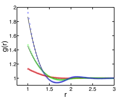
Figure 1: (Color online) The correlation function $g(r)$ computed from the PY equation (curves) and from Monte Carlo simulationswhitlock (symbols) in $d=4$. Results are plotted for $\rho=0.1$ ($\triangle$), $\rho=0.3$ ($\bigcirc$) and $\rho=0.5$ ($\square$). The PY results are plotted taking $10$ terms of the series (45)-(46) and were computed with $\mbox{$\Delta r$}=10^{-3}$.

Figures 1, 2 and 3 show $g(r)$ for $d=4,6$ and $8$, respectively with several different values of $\rho$. (The values of $\rho$ used here are chosen to be smaller than the radius of convergence of the virial series, see §VI.2 and §VI.3 below. For larger values of $\rho$, the series (45)-(46) does not converge, though it may perhaps be resummed to improve the convergence for larger densities.) We see that there is generally very good agreement in each case between the PY results (solid curves) and MC simulations (symbols). We note that, as expected, the discrepancy is largest for $r\approx 1$ — similar to the behavior observed in other dimensionslado ; PY2d . Interestingly, this discrepancy seems to diminish as the dimension increases. The good agreement between the MC results and our solutions of the PY equation shows that our method of solution works well.

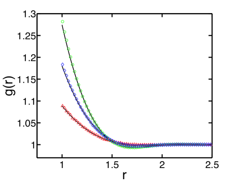
Figure 2: (Color online) The correlation function $g(r)$ computed from the PY equation (curves) and from Monte Carlo simulationswhitlock (symbols) in $d=6$. Results are plotted for $\rho=0.1$ ($\triangle$), $\rho=0.2$ ($\Diamond$) and $\rho=0.3$ ($\bigcirc$). The PY results are plotted taking $10$ terms of the series (45)-(46) and were computed with $\mbox{$\Delta r$}=10^{-3}$.

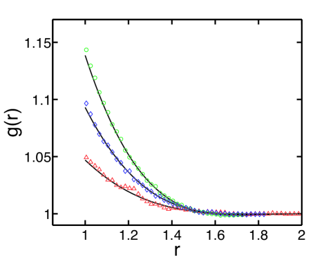
Figure 3: (Color online) The correlation function $g(r)$ computed from the PY equation (curves) and from Monte Carlo simulationswhitlock (symbols) in $d=8$. Results are plotted for $\rho=0.1$ ($\triangle$), $\rho=0.2$ ($\Diamond$) and $\rho=0.3$ ($\bigcirc$). The PY results are plotted taking $10$ terms of the series (45)-(46) and were computed with $\mbox{$\Delta r$}=10^{-3}$.

VI.2 Virial coefficients

We computed the virial coefficients using the two expressions (V) and (55) for $d=2$ as a check of our numerical scheme. (Note that this is not a trivial verification since the numerical scheme is completely different to that used previouslyPY2d .) We obtain the same results as reported previously PY2d , though our estimation of errors leads to some slightly different values for the last digit of the higher order coefficients.

The virial coefficients calculated by this method for $d=4,6$ and $8$ are reproduced in tables 2-4. These tables show the virial coefficients resulting from both the virial $(v)$ and compressibility $(c)$ routes, as well as the virial coefficients obtained by earlier MC calculationsclisby06 . Note that all the virial coefficients up to $B_{4}$ are known exactly (see Eq. (56) and Table 1 above), and agree with the MC calculations. In general, we see that $B_{i}^{(c)}$ is a better estimator of the true virial coefficient, $B_{i}^{(MC)}$, than $B_{i}^{(v)}$.

$i$	$B_{i}^{(v)}$	$B_{i}^{(c)}$	$B_{i}^{(MC)}$
3	$3.083$	$3.083$	$3.083$
4	$1.774$	$2.466$	$2.281$
5	$0.988$	$1.602$	$1.323$
6	$0.315$	$0.875$	$0.707$
7	$0.285$	$0.463$	$0.323$
8	$-0.103$	$0.193$	$0.161$
9	$0.278$	$0.120$	$0.061$
10	$-0.386$	$0.0046$	$0.038$
11	$0.642$	$0.071$	—
12	$-1.058$	$-0.076$	—
13	$1.793$	$0.134$	—
14	$-3.088$	$-0.210$	—
15	$5.402$	$0.348$	—

Table 2: Numerical values of the first fifteen virial coefficients in four dimensions. The $B_{i}^{(MC)}$ are the results from Monte Carlo calculations presented previously clisby06 . $B_{i}^{(v)}$ and $B_{i}^{(c)}$ are the values found from the solution to the PY equation using Eqs. (55) and (V) respectively.

$i$	$B_{i}^{(v)}$	$B_{i}^{(c)}$	$B_{i}^{(MC)}$
3	$2.276$	$2.276$	$2.276$
4	$0.189$	$0.795$	$0.576$
5	$0.51(7)$	$0.342$	$0.335$
6	$-0.72(2)$	$-0.104$	$-0.200$
7	$1.43(7)$	$0.278$	$0.389$
8	$-3.0(4)$	$-0.509$	$-0.688$
9	$6.8(6)$	$1.043$	$1.326$
10	$-16.(3)$	$-2.255$	$-2.696$
11	$40.(5)$	$5.097$	—
12	$-10(2)$	$-11.94(7)$	—
13	$26(5)$	$28.86(1)$	—
14	$-7(10)$	$-71.51(5)$	—
15	$19(15)$	$181.09(1)$	—

Table 3: Numerical values of the first fifteen virial coefficients in six dimensions. The $B_{i}^{(MC)}$ are the results from Monte Carlo calculations presented previously clisby06 . $B_{i}^{(v)}$ and $B_{i}^{(c)}$ are the values found from the solution to the PY equation using Eqs. (55) and (V) respectively.

$i$	$B_{i}^{(v)}$	$B_{i}^{(c)}$	$B_{i}^{(MC)}$
3	$0.966$	$0.966$	$0.966$
4	$-0.13(1)$	$0.065$	$-0.021$
5	$0.21(3)$	$0.074$	$0.126$
6	$-0.30(2)$	$-0.078$	$-0.155$
7	$0.5(1)$	$0.11(5)$	$0.239$
8	$-0.9(0)$	$-0.19(0)$	$-0.406$
9	$1.(7)$	$0.33(6)$	$0.747$
10	$-3.(4)$	$-0.6(4)$	$-1.466$
11	$7.(5)$	$1.(3)$	—

Table 4: Numerical values of the first eleven virial coefficients in eight dimensions. The $B_{i}^{(MC)}$ are the results from Monte Carlo calculations presented previously clisby06 . $B_{i}^{(v)}$ and $B_{i}^{(c)}$ are the values found from the solution to the PY equation using Eqs. (55) and (V) respectively.

We seem to see the same trends as Rohrmann et al.rohrmann08 regarding the way in which the PY virial coefficients bound the true virial coefficient for $d\geq 7$ (though our results reveal that the transition in behavior they observe occurs already at $d=6$, rather than $d=7$). In particular, we see that $B_{i}^{(v)}<B_{i}<B_{i}^{(c)}$ for even $i>4$ and $B_{i}^{(v)}>B_{i}>B_{i}^{(c)}$ for odd $i>5$.

Note also the intermediate behavior observed previouslyrohrmann08 for $d=5$ is observed already with $d=4$, though the details are a little different: we find that $B_{i}<B_{i}^{(c)}<B_{i}^{(v)}$ for odd $i>7$ and $B_{i}>B_{i}^{(c)}>B_{i}^{(v)}$ for even $i>8$ — though one would need to see more real virial coefficients to say this with more confidence.

VI.3 Convergence of virial series

A question of considerable interest is the radius of convergence of the virial series. This question is closely related to the nature of the singularity closest to the origin, which was addressed recently in odd dimensions rohrmann08 . An estimate of this radius of convergence may be made by using the Domb-Sykes plothinch ; vandyke . This is an extension of the ratio test in which the ratio between successive terms, $B_{i}/B_{i-1}$ is plotted as a function of $1/i$. Such a plot often reveals a linear behavior, the intercept of which then provides an estimate of the radius of convergence of the series, $\rho_{\mathrm{conv}}$, via

$$\rho_{\mathrm{conv}}^{-1}=\lim_{i\rightarrow\infty}\left|\frac{B_{i}}{B_{i-1}}\right|\,.$$ (58)

An example of such a plot is shown in Fig. 4 for the virial coefficients in six dimensions.

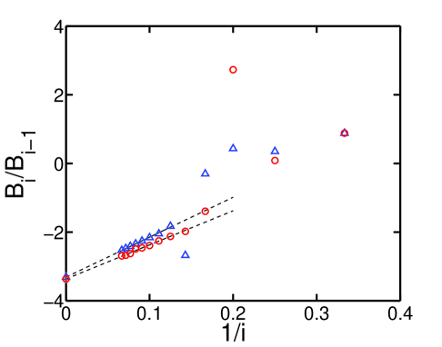
Figure 4: (Color online) Domb-Sykes plot for the virial coefficients in six dimensions. The ratios are based on the virial coefficients for $P^{(c)}$ ($\triangle$) and $P^{(v)}$ ($\bigcirc$). The dashed lines show the relevant linear fits at large $i$ and the points at the intersection with the $y$-axis shows the extrapolated limits and the associated error bars.

We used the Domb-Sykes plot to determine the radius of convergence of the series for $d=2,4,6$ and $8$. The results are given in table 5 as the radius of convergence for the series in $\eta$, $\eta_{\mathrm{conv}}$, along with estimates of the error in each case (Eq. (5) may be used to convert $\eta_{\mathrm{conv}}$ to $\rho_{\mathrm{conv}}$). These results are also plotted in Fig. 5 and combined with the results for odd dimensions $d\leq 13$ obtained by the analysis of Rohrmann et al.rohrmann08 . These results seem to confirm the assertion that as $d\rightarrow\infty$,

$$\eta_{\mathrm{conv}}\sim 2^{-d}\,,$$ (59)

which was conjectured by Frisch and Percus frisch for the full problem. The Domb-Sykes plots for $d=4,6,8$ have negative intercepts with the vertical axis and positive slopes there (see, Fig. 4, for example). This shows that, in these cases, the singularity that limits the radius of convergence of the virial series is a branch point on the negative real axisvandyke ; hinch . In contrast, the Domb-Sykes plot for two dimensions suggests that the relevant singularity is a pole on the positive real axis.

$d$	$\eta^{(v)}_{\mathrm{conv}}$	$\eta^{(c)}_{\mathrm{conv}}$
2	$1.008\pm 0.002$	$1.01\pm 0.002$
4	$0.146\pm 8\times 10^{-5}$	$0.150\pm 0.003$
6	$0.024\pm 7\times 10^{-4}$	$0.024\pm 6\times 10^{-4}$
8	$0.0055\pm 8\times 10^{-4}$	$0.0051\pm 5\times 10^{-4}$

Table 5: The radii of convergence for the virial series, for both the virial (v) and the compressibility (c) routes, as a function of the dimension $d$.

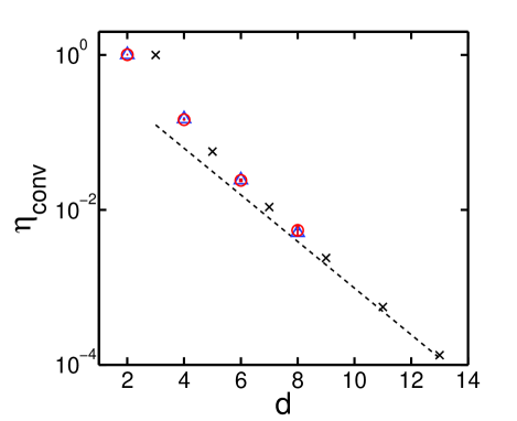
Figure 5: (Color online) The radius of convergence for the virial series, $\eta_{\mathrm{conv}}$, as a function of dimension, $d$. The radius of convergence in odd dimensions ($\times$) is taken from the work of Rohrmann et al.rohrmann08 . The results in even dimensions are found from the relevant Domb-Sykes plots and show estimates based on $P^{(c)}$ ($\triangle$) and $P^{(v)}$ ($\bigcirc$). The dashed line shows the relationship $\eta_{\mathrm{conv}}=2^{-d}$, which is believed to describe the large $d$ behavior of $\eta_{\mathrm{conv}}$.

VII Discussion

In this paper we generalized a semi-analytic method to solve the PY equation for hard discs PY2d to the case of hard hyperspheres in even dimensions. The essence of this approach is a reduction of the PY equation to a set of integro-differential equations for two auxiliary functions $Q(s)$ and $\psi(s)$ as given by Eqs. (33),(36) and (37). The correlation functions and the equation of state can be determined easily from these auxiliary functions. We suggest an efficient iterative numerical method to solve these equations and determine the auxiliary functions in $d=4,6$ and $8$. Using this method we are able to determine the values of the virial coefficients within the PY approximation and compare them with the first ten virial coefficients for the full problem clisby06 . We also obtain results for the pair correlation function which compare well with the available MC simulationswhitlock .

The principal advantage of this approach is that it provides directly the virial series, and so it yields the equation of state for all values of $\rho$ at the same time provided that $\rho<\rho_{\mathrm{conv}}$. This is in contrast with other approaches where each value of $\rho$ requires a separate calculationlado . An important consequence is that we can study the convergence of the series. We have shown that the virial series predicted by the PY theory for hyperspheres in even dimensions has a branch point on the negative real axis $\eta=-\eta_{\mathrm{conv}}$ for all $d\geq 4$. This is observed in both the virial and compressibility routes to determining the equation of state, similar to what happens in PY in odd dimensions rohrmann08 . The position of this singularity as a function of the the dimension $d$ is also consistent with the conjecture by Frisch and Percus frisch for the full problem in large dimensions. The successful prediction of the singularity supports the idea that the PY theory approaches the exact problem as the dimensionality increases. An important conclusion from this discussion is that semi-phenomenological equations of state, such as the generalizations of the celebrated Carnahan-Starling equation of state CarStar (for three-dimensional hard spheres) to higher dimensions Song , are inferior to the PY theory since they are not able to reproduce such a branch point singularity. This characteristic is also missing from far more elaborated equations of state Luban90 ; robles .

Another interesting prediction of the current work is that the exact virial coefficients $B_{i}$ for $d=4$ may change sign if they are computed for sufficiently large $i$. We observe that in PY theory with $d=4$ the virial coefficients determined by both routes are negative for even $i\geq 12$. This suggests that the exact coefficient may also become negative for sufficiently large $i$ and will hopefully motivate the calculation of further coefficients using the methods of Clisby and McCoyclisby06 . More generally the question of negative values of the virial coefficients in various dimensions is pertinentclisby04b ; clisby05 ; rohrmann08 .

As explained above, this method allows, in principle, calculations to arbitrary precision, and it could be interesting to obtain more virial coefficients by doing so. Such progress might also allow for a comparison of the pair correlation function with Molecular Dynamics simulations Lue05 ; Lue06 ; Skoge06 at large densities.

It could also be interesting to apply the approach developed here to polydisperse mixtures Lebowitz ; Baxter70 ; Gonzalez , to sticky hard spheres (i.e., hard spheres with an adhesive short range interaction) Baxter68 and to much higher dimensions.

Acknowledgments

We would like to thank Profs Whitlock and Bishop for sharing their data with us, and Prof. Santos for his useful comments. This work was supported by the Royal Commission for the Exhibition of 1851 (D.V.). Laboratoire de Physique Statistique is associated with Universities Paris VI and Paris VII.

Appendix A Numerical scheme

We solve the system of equations (47)-(50) by discretizing in space using steps of size $\Delta r$. Integrals are calculated using the trapezoidal rule, which is first order accurate. To calculate derivatives we developed two different schemes: one which used forward differencing (first-order accuracy) and the other using central differencing (second-order accuracy). The results obtained with these two differentiation schemes are consistent with one another. Iterations proceed from $i=0$ using the values for $\psi_{0}(t)$ and $q_{0}(t)$ from (47) to determine $\psi_{1}(t)$. The function $\psi_{1}(t)$ may then be used with the discretized version of (50) to determine $q_{1}(t)$. This process is then repeated $N$ times, corresponding to determining the first $N$ terms in the series expansions of $\psi(t)$ and $q(t)$. The results presented in this paper typically have $N=10$.

The virial coefficients were determined by numerical integration, again using the trapezoidal rule. To determine the values of these coefficients more accurately, we performed computations at different spatial resolutions, i.e.  with different values of $\Delta r$. Plotting the behavior of these numerically determined coefficients as a function of $\Delta r$ we then extrapolated the observed trend to $\mbox{$\Delta r$}=0$. The observed trend was linear for the scheme using differentiation by forward differencing, as expected since both discretizations involve errors of order $\Delta r$. The second scheme (using differentiation by central differencing) is more complicated since the first order error of integration is mixed with a second-order error in differentiation. Typically with this scheme we find errors that scale like $\mbox{$\Delta r$}^{3/2}$. In Fig. 6 below we show an example of the convergence using these two schemes.

Figure 6: (Color online) An example of the convergence of the virial coefficients as a function of $\Delta r$ for $B_{5}^{(c)}$ with $d=6$ using the two numerical schemes described in the text: forward differencing ($\square$) and central differencing ($\bigcirc$). For both data sets the dashed lines are the result of the fitting procedure, with a slope of $1$ for forward differencing, and with a slope of $3/2$ for central differencing. Note that the plot is on a log-log scale.

To determine the values presented in tables 2-4 we use the values extrapolated to $\mbox{$\Delta r$}=0$ from both numerical schemes. An estimate of the error introduced in this extrapolation procedure was obtained using the $95\%$ confidence interval for the value at $\mbox{$\Delta r$}=0$. The results presented in tables 2-4 are correct to $3$ decimal places or as otherwise indicated.

References

- (1) M. Bishop, P. A. Whitlock, and D. Klein, J. Chem. Phys. 122, 074508 (2005); M. Bishop and P. A. Whitlock, J. Chem. Phys. 123 , 014507 (2005); P. A. Whitlock, M. Bishop and J. L. Tiglias, J. Chem. Phys. 126, 224505 (2007); M. Bishop and P. A. Whitlock, J. Stat. Phys. 126, 299 (2007).
- (2) M. Skoge, A. Donev, F. H. Stillinger and S. Torquato, Phys. Rev. E 74, 041127 (2006).
- (3) L. Lue, J. Chem. Phys. 122, 044513 (2005).
- (4) L. Lue and M. Bishop, Phys. Rev. E 74, 021201 (2006).
- (5) N. Clisby and B. M. McCoy, J. Stat. Phys. 122, 15 (2006).
- (6) N. Clisby and B. M. McCoy, J. Stat. Phys. 114, 1343 (2004); I. Lyberg, J. Stat. Phys. 119, 747 (2005).
- (7) M. Luban and A. Baram, J. Chem. Phys. 76, 3233 (1982); M. Baus and J. L. Colot, Phys. Rev. A 36, 3912 (1987).
- (8) N. Clisby and B. M. McCoy, J. Stat. Phys. 114, 1361 (2004).
- (9) N. Clisby and B. M. McCoy, Pramana-J. Phys. 64, 775 (2005).
- (10) R. D. Rohrmann and A. Santos, Phys. Rev. E 76, 051202 (2007).
- (11) R. D. Rohrmann, M. Robles, M. López de Haro and A. Santos, J. Chem. Phys. 129, 014510 (2008).
- (12) M. Robles, M. L. de Haro, and A. Santos A, J. Chem. Phys. 120, 9113 (2004); Erratum 125 219903(E) (2006); J. Chem. Phys. 126, 016101 (2007).
- (13) H. L. Frisch and J. K. Percus, Phys. Rev. A, 35, 4696 (1987); H. L. Frisch and J. K. Percus, Phys. Rev. E, 60, 2942 (1999).
- (14) P. M. Chaikin and T. C. Lubensky, Principles of Condensed Matter Physics (Cambridge University Press, Cambridge, United Kingdom, 1995).
- (15) S. Torquato, Random Heterogeneous Materials: Microstructure and Macroscopic Properties. NewYork: Springer-Verlag, 2002.
- (16) S. Torquato and F. H. Stillinger, Experimental Mathematics 15, 307 (2006).
- (17) J. H. Conway and N. J. A. Sloane, Sphere Packings, Lattices and Groups (Springer-Verlag, New York, 1993).
- (18) J. K. Percus, and G. J. Yevick, Phys. Rev. 110, 1 (1958).
- (19) L. S. Ornstein, and F. Zernike, Proc. Acad. Sci. Amsterdam 17, 793 (1914).
- (20) S.F. Edwards and M. Schwartz, J. Stat. Phys. 110, 497 (2003).
- (21) R. J. Baxter, Aust. J. Phys. 21, 563 (1968).
- (22) E. Leutheusser, Physica A 127, 667 (1984).
- (23) E. Leutheusser J. Chem. Phys. 84, 1050 (1986).
- (24) M. S. Wertheim, J. Math. Phys. 5, 643 (1964).
- (25) M. S. Wertheim, Phys. Rev. Lett. 10, 321 (1963).
- (26) E. Thiele, J. Chem. Phys. 39, 474 (1963).
- (27) Y. Rosenfeld, J. Chem. Phys. 87, 4865 (1987).
- (28) J. P. Hansen, and R. McDonald, Theory of simple liquids (Academic Press, New York, 2006).
- (29) F. Lado, J. Chem. Phys. 49, 3092 (1968).
- (30) W. G. Hoover and B. J. Alder, J. Chem. Phys. 46, 686 (1967).
- (31) D. G. Chae, F. H. Ree, and T. Ree, J. Chem. Phys. 50, 1581 (1969).
- (32) B. J. Alder, W. G. Hoover, and D. A. Young, J. Chem. Phys. 49, 3688 (1968).
- (33) W. W. Wood, J. Chem. Phys. 52, 729 (1970).
- (34) M. Abramowitz, and I. A. Stegun (Eds.), Handbook of Mathematical Functions with Formulas, Graphs, and Mathematical Tables (Dover, New York, 1972).
- (35) M. Adda-Bedia, E. Katzav, and D. Vella, J. Chem. Phys. 128, 184508 (2008); Erratum, 129, 049901 (2008).
- (36) I. N. Sneddon The Use of Integral Transforms (McGraw Hill, 1972).
- (37) I. S. Gradshteyn and I. M. Rhyzik Table of Integrals, Series, and Products (Academic Press, New York, 2007).
- (38) J. L. Lebowitz, Phys. Rev. 133, A895 (1964).
- (39) M. González-Melcho, J. Alejandre and M. Loṕez de Haro, J. Chem. Phys. 114, 4905 (2001).
- (40) R. J. Baxter, J. Chem. Phys. 52, 4559 (1970).
- (41) R. J. Baxter, J. Chem. Phys. 49, 2770 (1969).
- (42) M. van Dyke, Q. J. Mech. Appl. Math. 27, 423 (1974).
- (43) E. J. Hinch Perturbation Methods (Cambridge University Press, Cambridge, 1991).
- (44) N. F. Carnahan and K. E. Starling, J. Chem. Phys. 51,635 (1969).
- (45) Y. Song, E. A. Mason, and R. M. Stratt, J. Phys. Chem. 93, 6916 (1989); Y. Song and E. A. Mason, J. Chem. Phys. 93, 686 (1990).
- (46) M. Luban and J. P. J. Michels, Phys. Rev. A, 41, 6796 (1990).