Improved Algorithms for Approximate String Matching (Extended Abstract)
Abstract
Background:
The problem of approximate string matching is important in many different areas such
as computational biology, text processing and pattern recognition. A great effort has
been made to design efficient algorithms addressing several variants of the problem,
including comparison of
two strings, approximate pattern identification in a string or
calculation of the longest common subsequence that two strings share.
Results:
We designed an output sensitive algorithm solving the edit distance problem between two strings of
lengths and respectively in
time and linear space, where is the edit distance
between the two strings. This worst-case time bound sets the quadratic factor of the algorithm
independent of the longest string length and improves existing theoretical bounds for this problem.
The implementation of our algorithm excels also in practice, especially in cases
where the two strings compared differ significantly in length.
Conclusions:
We have provided the design, analysis and implementation of a new algorithm for calculating the edit distance of two strings with both theoretical and practical implications. Source code of our algorithm is available at http://www.cs.miami.edu/~dimitris/edit_distance.
Background
Approximate string matching is a fundamental, challenging problem in Computer Science, often requiring a large amount of computational resources. It finds applications in different areas such as computational biology, text processing, pattern recognition and signal processing. For these reasons, fast practical algorithms for approximate string matching are high in demand. There are several variants of the approximate string matching problem, including the problem of finding a pattern in a text allowing a limited number of errors and the problem of finding the number of edit operations that can transform one string to another. We are interested in the latter form in this paper.
The edit distance between two strings and is defined in general as the minimum cost of any sequence of edit operations that edits into or vice versa. In this work we will focus on the Levenshtein edit distance [1], where the allowed edit operations are insertion, deletion or substitution of a single character, with each operation carrying a cost of . This type of operation is often called unit-cost edit distance and is considered the most common form. The weighted edit distance allows the same operations as the Levenshtein edit distance, but each operation may have an arbitrary cost.

In the literature there exist a number of algorithms dealing with the calculation of the edit distance between two strings. The basic dynamic programming algorithm that solves the problem in time and linear space has been invented and analyzed several times in different contexts [2, 3, 4, 5, 6, 7], published between 1968 and 1975. Early on there was an algorithm by Masek and Paterson [8], building on a technique called the ”Four-Russian paradigm” [9], which computes the edit distance of two strings over a finite alphabet in time . This algorithm is not applicable in practice, since it can outperform the basic algorithm only then the input size is exceeding 40GB. All these algorithms can also be used to calculate the alignment of two strings, in addition to their edit distance. A modification of the basic algorithm by Hirschberg [10] allows the alignment calculation to be performed using linear space as well.
A few years later in 1985, Ukkonen arrived at an time algorithm, using space [11], where is the edit distance of the two strings compared, creating a very efficient output sensitive algorithm for this problem. The following year, Myers published an algorithm for the Longest Common Substring (LCS) problem, which is similar to the edit distance problem, which has time and linear space complexity [12]. In achieving this result, a generalized suffix tree of the input strings, supplemented by Lowest Common Ancestor (LCA) information, has to be used, which renders the solution impractical and only of theoretical value. The practical version of that algorithm needs time. From the other hand, a variation of Ukkonen’s algorithm using space leads to an efficient, straightforward implementation, using recursion. Lastly, the basic algorithm, although theoretically inferior, is the most commonly used, owing to its adaptability, ease of implementation, instruction value, and speed, the latter being a result of low constant operations.
In this paper we will present an time and linear space algorithm to calculate the edit distance of two strings, which improves on all previous results, the implementation of which is practical and competitive to the fastest algorithms available. The quadratic factor in the time complexity now becomes independent of the longest string, with the algorithm performing its best when the two strings compared differ significantly in size.
Methods
Definitions
In this section we closely follow the notation and definitions in Ref. [11]. Let and be two strings of lengths and respectively, over a finite alphabet . Without loss of generality, let .
To define the edit distance between two strings and , we will let the possible editing operations be deletion, insertion and substitution. Then we define edit distance as the minimum number of character insertions, deletions and substitutions to transform string to string . By that definition, each editing operation has a cost of and this edit distance in bibliography is usually referred to as Levenshtein edit distance [1]. Edit operations can be generalized to have non-negative costs, but for the sake of simplicity in the analysis of our algorithm we will concern ourselves only with the Levenshtein edit distance. We also assume that there is always an editing sequence with cost converting into such that if an cell is deleted, inserted or changed, it is not modified again. Under these assumptions the edit distance is symmetric and it holds . Since and there is a minimum number of indels that need to be applied in transforming into , the last equation becomes . The insertion and deletion operations are symmetric, since an insertion, when transforming to , is equivalent to a deletion in the opposite transformation, and vice versa. Both operations will be referred to as indels.
The basic dynamic programming algorithm employed to solve the edit distance problem, invented in a number of different contexts [2, 3, 4, 5, 6, 7], makes use of the edit graph, an matrix that is computed from the recurrence:
| min( | If then else , | ||
| , | |||
| , or . |
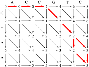
This matrix can be evaluated starting from and proceeding row-by-row or column-by-column. This process takes time and space and produces the edit distance of the strings in position . The cells of the matrix (nodes of the graph) have dependencies based on this recurrence, forming the dependency or edit graph, a directed acyclic graph that is shown in Fig.1. All edit graph nodes will be referred to as cells and all graph edges (edit operations) will be referred to as transitions.
To refer to the diagonals of we number them with integers such that the diagonal denoted by consists of those cells for which . The diagonal , where the final value resides, is special for our purposes and we will call it main diagonal. The matrix cells between diagonals and (inclusive) consist the center of the edit graph/matrix, the lower left triangle between diagonals to will be called the left corner of the graph and upper right triangle between diagonals and will be called the right corner of the graph.
A path in the edit graph is a series of transitions connecting cells, similar to a path in a directed graph. Whenever we generally refer to a path, we will assume that the final cell it reaches is . The optimal path will be a path originating at , and for which the sum of the costs of its transitions is minimal among all paths from .
The concept

The basic dynamic programming algorithm evaluates unnecessary values . This observation led Ukkonen [11] design an algorithm that is diagonal-based and computes cell values only between the diagonals and . He also used the observation that, under the edit operations’ cost scheme discussed previously, the values in a diagonal are monotonically increasing, where for Levenshtein edit distance costs it is furthermore .
Both Ukkonen [11], for calculating the edit distance, and Myers [12], for calculating the length of the Longest Common Substring (LCS) of two strings, a problem closely related to the edit distance, designed their algorithms with a common feature: The iterations in evaluating the edit graph cells were score based, as opposed to column or row based in the basic algorithm. In each step they would increase the edit distance by , starting at , and evaluate all cells with values , meaning cells reachable with edit distance , often omitting cells not contributing to the next iteration, by considering transitions between cells where the values are incremented.
The algorithm we present here builds on all previous observations and the main iteration is score based as well. But we also make use of the following facts:
-
1.
A number of indels () is unavoidable when the two strings considered differ in size.
-
2.
Additional indels are unavoidable when the optimal path strays away from the main diagonal.
-
3.
Certain cells do not contribute to the optimal path or their contribution is redundant.
The first point is obvious, since the optimal path, starting at diagonal and ending at diagonal , can only use indels to progress through diagonals. To argue towards the second fact we notice that every time a path follows an indel from diagonal to when or from diagonal to when , that path will need to follow another compensatory indel at some later point, in order to reach the main diagonal, where the target cell resides.
In order to address the third fact, we will introduce the concept of dominance. We will say that cell dominates cell if no path through defines a better edit distance than the optimal path through . This implies that has an equal or better potential to belong to the optimal path (which defines ) than , and thus the latter and its paths do not need to be considered further.
Some dominance relations between cells can be spotted easily. Let us consider all possible paths starting from . If a match exists between characters and (), then we do not need to consider indel transitions from to and . In that case actually, all cells for and for are dominated by . Since matches , cell obtains the value of . Then all cells , can obtain a value of through a path traversing . Any path through cannot result in a smaller value for cells , , since cells have the same value. In a similar manner, cells in the second column starting at the third line are dominated by . These arguments apply not only to but to all in general, proving the following:
Lemma 1.
A cell is dominated by if .
Let us now consider what happens when . In this case we can still find dominated cells in the second row and column, depending on the first matching character position in each. Let us assume that the first character in matching is , . All cells , are dominated by , for the same reasons that were described earlier. And a similar domination relation exists in the columns.
Before we generalize the dominance relation through a theorem, we will introduce a new scoring scheme to take advantage of the indel unavoidability, which will create another optimization criterion, monotonicity in the rows and columns of certain parts in our graph. For the new scoring scheme and for the rest of the description of our algorithm, we will divide our matrix into two parts, separated by the main diagonal. The first part includes the center and the left corner of the matrix, where the second part includes the right corner of the matrix, together with the main diagonal (which is shared by both parts). The scoring scheme and the algorithm described further on will be analyzed on the part of the matrix left of the main diagonal, although all theory works symmetrically on the part right of the main diagonal, by substituting the rows with columns and vice versa.
The new scoring scheme, for the left part of the matrix, is implemented as follows: Every vertical transition (indel) incurs a cost of , since it strays away from the main diagonal and creates the need of another horizontal indel to compensate. All horizontal transitions do not carry any cost. The match and substitution costs remain and respectively. To obtain the edit distance , we add to the value of cell . The transformation is illustrated through an example in Fig. 2.
To guarantee the correctness of an algorithm based on that scoring scheme, we will now prove the following lemma:
Lemma 2.
Under the new scoring scheme, the edit distance of and remains unchanged.
Proof.
It has already been shown that the edit distance is defined by an optimal path of the fewest possible edit operations carrying a cost, resulting in the minimum score at . We will prove the following two statements:
-
1.
The score obtained from the optimal path remains unchanged and
-
2.
No other path can lead to a sequence of fewer edit operations and thus a smaller score / edit distance.
To prove the first statement, we note the following: The number of match and substitution transitions in the optimal path do not alter the edit distance in the new scoring scheme, since the costs of these operations have not changed. With the optimal path starting at diagonal and ending at diagonal , there are indels which can be omitted from our calculation, since with the new scoring scheme we add these at the end. The only remaining edit operations to examine are vertical indels left of the main diagonal and horizontal indels right of the main diagonal, which must be accompanied by compensatory horizontal and vertical indels in the respective parts, or the optimal path cannot end up in the main diagonal. Since these indels come in pairs, with half of them carrying the cost of and half the cost of in the new scoring scheme, the final edit distance remains unchanged.
The second statement follows from the previous arguments, since any path under the new scoring scheme carries the same cost as before, so a new path with a better score than the previous optimal path score contradicts the optimality of the latter under the original scoring scheme. ∎
Since with the new scoring scheme horizontal transitions do not carry a cost, the values of cells in every row in the left part of the matrix are monotonically decreasing. The same holds for the columns in the right part of the matrix, which leads to the following:
Corollary 1.
Under the new scoring scheme, the values of cells in rows left of the main diagonal and in columns right of the main diagonal are monotonically decreasing as the indices of the corresponding cells increase.
Let us now consider all cells in a specific row , left of the main diagonal. Values on this row are monotonically decreasing and we only need to keep the information of the first cells from the right where the values are changing (the leftmost cells of a series of cells with the same value), since the rest of the cells are dominated (can be reached with cost from the aforementioned cells). Now, if we have two consecutive dominant cells and on row , with and , then the value of can be propagated through a transition to row only if a match exists between and , with . In order to be able to locate such matches in constant time, we will create lookahead tables for each letter of the alphabet , which can point to the next matching character from strings and . Basically these lookahead tables will be able to answer the question: Given a character and a position , what is the smallest index such that ? And the same for string . Such a lookahead table can be easily constructed in time and space , which for a fixed alphabet of constant size is linear, by traversing both strings in reverse order, once for each character of the alphabet.
One can easily verify that lemma 1 still holds, based on the same arguments used to prove it, under the new scoring scheme. In addition, the following corollary holds:
Corollary 2.
A cell with value dominates all cells , with values .
Proof.
It is easy to see, with a simple inductive argument, that a cell dominates all parental cells on the same diagonal with the same score. Since any cell dominates itself with a higher score (because every path from that cell will have a higher score equal to the difference of the two scores), the corollary follows. ∎
The algorithm
The algorithm works separately on the two parts of the matrix left and right of the main diagonal. For the description of the algorithm will consider only the part of the matrix lying left of the main diagonal, with the assumption that all operations are symmetric on the right part of the matrix. An exception will occur when we describe the interface of the two parts.
Our edit distance algorithm is score based. On each iteration the edit distance score is incremented by and the part of the edit graph that can be reached with the current score is determined. The initial score is , although we should keep in mind that, since at the end we add to the score – adjusting for the unavoidable indels that we get for free on horizontal transitions – it can be considered as if the score is initialized with the value .
During each iteration, we keep the values and positions of the cells we work with in a double linked list, which will be referred to simply as list. To store the position of a cell we actually need only the column index where the cell resides, for reasons that will be explained later. The initialization phase starts with the determination of the cells which can be reached with a score of . Since all horizontal and match diagonal transitions (diagonal transitions corresponding to matching characters) have a cost of , we follow horizontal transitions until we locate a match, then advance to the next line and repeat. The process ends when we reach the main diagonal. We do not need to keep information on all cells with value, the first cell with a value of on each line suffices, since all further cells are dominated. These dominant leftmost cells can be located in constant time for each line, by using the lookahead tables. When we encounter a series of matches on the same diagonal, we only need to keep the value of the last (bottom-right) cell, since all other cells are dominated. The indices of cells accessed through this process increase monotonically, as we advance forward through rows, columns and diagonals. The initialization finishes when the main diagonal is reached. Thus at the end of the initialization step we have a list of cells with value, each of which resides on a different row, column and diagonal of the matrix. An example of the initialization phase can be found in Fig. 3a.
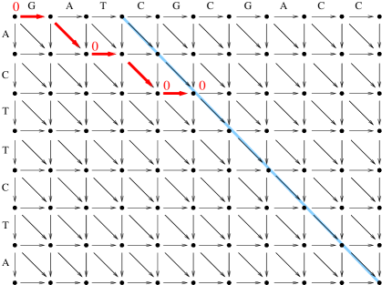
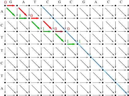
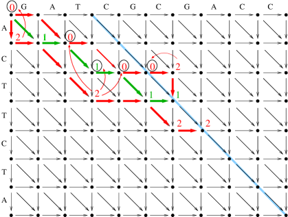
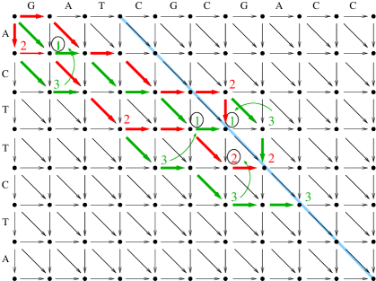
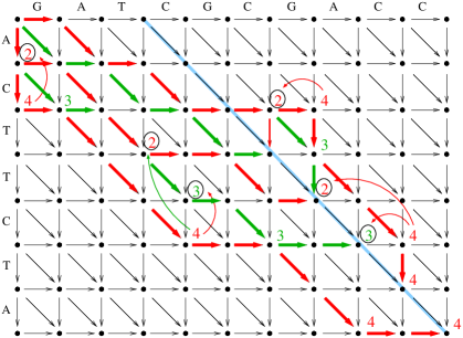
On each subsequent iteration of the algorithm and with each increasing value of the score, the linked list is updated with new cells that can be reached from members of the list. The algorithm at iteration , with also being the current score, starts from the top of the list and processes one cell at a time. For each list cell examined having a value of or , as will be proved in lemma 3, we either follow a substitution transition, if the cell’s value is or a vertical indel transition if the cell’s value is . Lets assume we are examining list cell . We know that , since if it would already be included in the list, unless dominated by another cell in the list, which is impossible since then would in turn be dominated by and would not be in the list during the current iteration. We now find the largest for which , and insert cell in the list. That is the last cell in a series of match transitions, starting at , if any exist. Next, we examine the cells following in the list and remove the ones that are dominated by . At this step, list cells in rows and on diagonals such that are removed, all being dominated as proved later in theorem 1. Starting now at cell , we repeat the process performed in the initialization, with the difference that for each new cell inserted in the list, all subsequent cells in the list that are dominated by the new member are removed. This process will stop once the next identified match in the lookahead table falls inside the dominated area. Precisely, if is the last cell with value that was inserted in the list, the next match from the lookahead tables resides at diagonal and the next cell in the list resides at a diagonal and row , then the process of inserting new cells derived from is terminated and we proceed to the next cell in the list.
Each iteration finishes once we reach the main diagonal. The reader can follow the procedure, through the five iterations in calculating the edit distance of strings ’GATCGCGACC’ and ’ACTTCTA’, in Fig. 3.
One special case that was not covered in the above description is the handling of a cell insertion following a vertical indel transition, when another dominated cell on the same diagonal exists in the list. In this case, the only position the dominated cell can occupy is previous to the current cell examined, from which the transition emanated. This results in the removal of the dominated cell. This special case only requires a constant number of operations and does not alter the complexity of the algorithm.
As already mentioned, the part of the matrix right of the main diagonal is processed in a symmetric way. At the end of each iteration, the cells of the main diagonal, which belongs to both parts, have to be updated. These cells reside at the end of the lists for both parts and the update is performed in constant time as well.
We will now proceed to prove the following theorem:
Theorem 1.
Cell on diagonal with value dominates all cells in the list with , and values , meaning all list cells in rows above it and columns with larger indices.
Proof.
Since horizontal transitions carry a cost of , all cells in row and column with have a score of at most . All cells in the list, residing in diagonals with and in rows with lead diagonal transitions to cells with score at most , since (or would not belong to the list, dominated by ). This implies that no diagonal transition from these cells can produce a value smaller than in any cell on row and column via a path passing through these cells, since values in the paths are monotonically increasing (because all edit operations have non-negative costs). If we now examine the vertical transitions emanating the cells under consideration, they also result in paths propagating scores at least , which again cannot result in a better score on the cells on row and column . All cells on diagonals do not need to be considered, since they cannot be reached from the claimed dominated cells of this theorem, unless a path reaches them through a cell in diagonal . But in corollary 2 we showed that cells on this diagonal with scores are already dominated by . Thus all cells are dominated by . ∎
The next corollary follows from the domination theorem 1:
Corollary 3.
No two cells in the list reside on the same column.
Proof.
Before a new candidate cell is inserted in the list, any list cell on the same column will be removed, since it is dominated by the newly inserted cell, based on the previous theorem. ∎
Now we have the necessary tools to prove the following lemma:
Lemma 3.
When iteration starts, with , all cells in the linked list have either a score of or .
Proof.
Initially, after the initialization, the list holds cells with value , so the lemma holds. Every time a cell is inserted in the list it will remain until it is dominated by another cell or the algorithm terminates. Unless a cell with score in the list is dominated and removed before its transitions are examined, when the algorithm reaches that cell the diagonal transition emanated from the cell will produce the next candidate, with score , to be inserted in the list. The second time this cell is visited, the vertical transition from it will be examined. In that case, the next candidate with score will dominate the current cell, according to the previous theorem. Thus, even if a cell is not dominated by another inserted cell, it will be dominated by its siblings. ∎
A direct consequence of the previous lemma is the following:
Corollary 4.
At most two cells in the list reside in the same diagonal, and their values differ by . This holds for same row list cells as well.
A pseudo-code description of the algorithm is presented below. The description excludes special cases requiring substitutions of the currently examined cells of the list and only presents the operations of the algorithm in the part of the matrix left of the main diagonal. The procedure interfacing the left and right linked lists is omitted as well. The code can be studied in more detail from the available code.
Algorithm complexity
The algorithm described in the previous section is score based and as such the main loop executes an equal number of times with the value recorded at cell of the edit graph. Since we add the value to that score in order to obtain the edit distance of strings and , the total number of iterations is equal to .
At all times during the execution of the algorithm the linked list contains at most cells, which is a direct consequence of corollary 3. Also, due to corollary 4, there can be at most cells in the list at any given time, since the maximum number of diagonals on which the algorithm processes cells is , consisting of the center of the matrix and diagonal bands of size from each side of the center, accessed while the algorithm iterates. Basically, for every two iterations of the algorithm, one further diagonal from each side of the center of the matrix is accessed.
All cells in the list are accessed in order and without backtracking during each iteration. Each cell undergoes through a constant number of structural accesses, once when it is inserted in the list, once when it is removed and two times when the diagonal and vertical transitions from this cell are examined, if there is a chance before it is dominated. During each iteration there are other cells accessed, the candidates for insertion in the list. While processing these cells we are advancing both the indices of columns and rows without backtracking, which proves, as with list cells, that there are at most or candidate cells examined during each iteration.
A candidate cell may be accessed several times while compared to a list cell, in order to determine a dominance relation. A list cell can also be accessed several times during the same process, to check whether it is dominated. The amortized cost for each cell though is constant. Every time a candidate cell is re-examined, a cell from the list has been removed. And every time a list cell is re-examined, in the previous step it was not dominated by a candidate cell, the latter then having being inserted in the list and not being examined again on that iteration. Since each time we advance through either a candidate or a list cell, and since both sets have cells (under the assumption that ), the total number of constant time operations during an iteration is .
This analysis demonstrates that the total running time of our algorithm is , where the last linear component represents the time necessary to initialize the lookahead tables. It can be easily verified using simple algebra that , which provides another less tight upper bound of the worst case time behavior of the algorithm, . We can therefore observe that the quadratic factor in the time complexity is independent of the longest string being compared. The space usage of this algorithm is , dominated by the size of the lookahead tables kept in memory. This completes the proof of the next theorem:
Theorem 2.
The edit distance of two strings and with lengths and respectively can be computed in time and in space .
Results
We have implemented our new algorithm to test its performance in practice. For comparison purposes, we implemented the basic algorithm, also known as Needleman-Wunsch [3], as well as the Ukkonen algorithm [11]. All algorithms were implemented in perl, using the same input/output procedures and no optimizations. Benchmarking was performed with the benchmark perl module for the experiments averaging a large number of random runs, and the time unix command for individual experiments, the same method always used across algorithms. All tests were performed on an 8GB RAM 2.93GHz Intel processor IBM compatible desktop machine, running ubuntu linux. In all test cases the data completely fit in the main memory.
Since perl does not support pointer structures efficiently, we implemented the double linked list with arrays, using the fact that no two cells in the list can reside on the same column. This way we access list cells using their column index. As such, the list occupies more space than the minimum possible, where the implementation may have been more efficient in another programming language supporting these structures.
Ukkonen’s algorithm implementation was based on the outline found in [11] and the more detailed description found in [13]. The version used is particularly simple by making use of recursion, but has larger than linear space demands, specifically . The basic algorithm was implemented using linear space and row-by-row iterations.
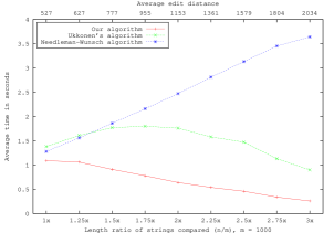
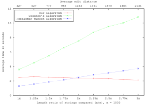
The first two experiments were run on random sequences over alphabets of and characters respectively, similar to random DNA/RNA and amino acid sequences. The length of the first sequence from the two compared was set at characters, where the length of the second sequence varied between and characters. We examined a total of nine length ratios values between and (). For each length ratio, different comparisons were run, with the execution time and edit distance values averaged among these. The results are depicted in Fig. 4.
| Sequence A | Sequence B | Alphabet | (Average) | Our | Ukkonen’s | Basic | (Average) |
| size | length | algorithm | algorithm | algorithm | edit | ||
| (sec) | (sec) | (sec) | distance | ||||
| Random 16S | Random 16S | 4 | 1350 | 0.679 | 0.811 | 2.554 | 421.3 |
| rRNA sequence | rRNA sequence | ||||||
| Hyphomonas 16S | Hyphomonas 16S | 4 | 1330 | 0.25 | 0.18 | 2.14 | 46 |
| rRNA (AF082798) | rRNA (AF082795) | ||||||
| Alphaproteobacteria 16S | Betaproteobacteria 16S | 4 | 1320 | 0.42 | 0.46 | 2.07 | 318 |
| rRNA (AJ238567) | rRNA (AJ239278) | ||||||
| Cucumber necrosis | Lisianthus necrosis | 4 | 4790 | 6.70 | 6.32 | 28.27 | 1154 |
| virus genome | virus genome | ||||||
| Human poliovirus 1 | Human Rhinovirus A | 20 | 870 | 1.02 | 1.05 | 0.88 | 472 |
| virion protein | virion protein |
In these simulations it is worth noticing significant performance improvement of the new algorithm with increasing length ratio of the random strings, although the total length of the strings is increasing. This is not surprising, since the number of iterations is decreasing, caused by a slower increase in edit distance than difference between the lengths of the two strings.
Ukkonen’s algorithm is under-performing when comparing random strings over a large alphabet, because of the large expected edit distance value in these cases. This algorithm is designed for comparing similar strings, which is the case most often encountered in practice. In contrast, the basic algorithm, owing to its simplicity, is performing consistently and surpassing the other algorithms when the edit distance is large compared to string length, unless when the value becomes small enough, where our algorithm takes the lead.
Next, we designed computational experiments performing comparisons most often encountered in practice, drawn from the computational biology domain. In all examples the sequence pairs examined have comparable lengths, not differing more than . The results are presented in Table 1. The first simulation involved random sequence pair comparisons from a pool of approximately 6800 vetted 16S ribosomal RNA sequences, provided by the Ribosomal Database Project (RDP) at http://rdp.cme.msu.edu. These sequences average about characters in size, drawn from an alphabet of size . A random pair of 16S rRNA sequences from the same genus and another from the same class but different order are compared in the next two lines, followed by a comparison of two viral genomes and two virion proteins.
As these results demonstrate, the performance of our algorithm compares favorably to Ukkonen’s asymptotically slower but with lower constants algorithm, while the basic algorithm is outperformed in almost every case, except when matches are sparse. Performance comes with some cost though and it is interesting to note that the size of the program implementations of the three algorithms, the basic, Ukkonen’s and ours, is , and lines of code respectively.
The perl implementations of all three algorithms used in this paper for performance comparisons can be downloaded at http://www.cs.miami.edu/~dimitris/edit_distance.
Conclusions
In this paper we have provided the design, analysis and implementation of a new algorithm for calculating the edit distance of two strings. This algorithm is shown to have improved asymptotic time behavior, while it is also demonstrated to perform very well in practice, especially when the lengths of the strings compared differ significantly. The performance of our algorithm in this case, which is encountered less often in instances of the edit distance problem, could find application in the related Longest Common Subsequence (LCS) and other similar problems solved with dynamic programming techniques.
Future directions for this algorithm include the investigation of further practical applications of the techniques described in other similar problems, as well as generalizing the results for arbitrary weights of the edit operations and/or covering additional edit operations such as swaps.
Acknowledgements
We would like to thank Gonzallo Navarro, Amihood Amir and Gad M. Landau for information provided regarding the complexity of the edit distance problem.
References
- [1] Levenstein V: Binary codes capable of correcting spurious insertions and deletions of ones. Probl. Inf. Transmission 1965, 1:8–17.
- [2] Vintsyuk T: Speech discrimination by dynamic programming. Cybernetics 1968, 4:52–58.
- [3] Needleman S, Wunsch C: A general method applicable to the search for similarities in the amino acid sequences of two proteins. J. Mol. Biol. 1970, 48:444–453.
- [4] Sankoff D: Matching sequences under deletion/insertion constraints. In Proceedings of the National Academy of Sciences of the USA, Volume 69 1972:4–6.
- [5] Sellers P: On the theory and computation of evolutionary distances. SIAM J. Appl. Math 1974, 26:787–793.
- [6] Wagner R, Fisher M: The string to string correction problem. J. ACM 1974, 21:168–178.
- [7] Lowrance D, Wagner R: An extension of the string-to-string correction problem. J. ACM 1975, 22:177–183.
- [8] Masek W, Paterson M: A faster algorithm for computing string edit distances. J. Comput. Syst. 1980, 20:18–31.
- [9] Arlazarov VL, Dinic EA, A KM, Faradzev IA: On economic construction of the transitive closure of a directed graph. Soviet Math. 1970, 11 (5):1209–1212.
- [10] Hirschberg DS: A Linear Space Algorithm for Computing Maximal Common Subsequences. Communications of the ACM 1975, 18 (6):341–343.
- [11] Ukkonen E: Algorithms for approximate string matching. Information and Control 1985, 64:100–118.
- [12] Myers EW: An O(ND) difference algorithm and its variations. Algorithmica 1986, 1:251–266.
- [13] Powell DR: Algorithms for Sequence Alignment. PhD thesis, Monash University, School of Computer Science and Software Engineering 2001.