Magnetic Flux Loss and Flux Transport in a Decaying Active Region

Abstract

We estimate the temporal change of magnetic flux perpendicular to the solar surface in a decaying active region by using a time series of the spatial distribution of vector magnetic fields in the photosphere. The vector magnetic fields are derived from full spectropolarimetric measurements with the Solar Optical Telescope aboard Hinode. We compare a magnetic flux loss rate to a flux transport rate in a decaying sunspot and its surrounding moat region. The amount of magnetic flux that decreases in the sunspot and moat region is very similar to magnetic flux transported to the outer boundary of the moat region. The flux loss rates [$(dF/dt)_{loss}$] of magnetic elements with positive and negative polarities are balanced each other around the outer boundary of the moat region. These results suggest that most of the magnetic flux in the sunspot is transported to the outer boundary of the moat region as moving magnetic features, and then removed from the photosphere by flux cancellation around the outer boundary of the moat region.

1 INTRODUCTION

How and where is magnetic flux in sunspots removed from the photosphere? Sunspot umbrae are sometimes split by formation of a light bridge, which is a bright lane crossing the umbra (Bray & Loughhead, 1964). Small magnetic features with a typical size less than 2$\arcsec$ called moving magnetic features (MMFs; Harvey & Harvey, 1973) are generally observed in the moat region that surrounds a decaying, mature sunspot. It has been reported that MMFs appear not only in the decaying phase of sunspots but also in the growing phase (e.g. Wang et al., 1991). The MMFs mostly appear around the outer boundary of the sunspot, moving almost radially outward during their lifetime ranging from a few minutes to 10 hr (Harvey & Harvey, 1973; Zhang et al., 2003; Hagenaar & Shine, 2005). The formation of the light bridges and MMFs is closely related to the fragmentation and disintegration of the sunspot magnetic flux. Indeed, it has been observed that the net flux carried away from the sunspot by MMFs is larger than the flux decrease in the sunspot (Martínez Pillet, 2002; Kubo et al., 2007). This indicates that MMFs can be responsible for the flux loss of the sunspot.

The mutual apparent loss of magnetic flux is often observed in the line-of-sight magnetograms when one magnetic polarity element collides with another polarity magnetic element in the photosphere. This apparent flux loss is called “magnetic flux cancellation” as a descriptive term. It is observed that moving magnetic features often collide with apparently static opposite polarity magnetic features around the outer boundary of the moat region (Martin, Livi, & Wang, 1985; Yurchyshyn & Wang, 2001; Chae et al., 2004; Bellot Rubio & Beck, 2005) and widely believed that understanding the flux cancellation process around the moat boundary is the key to understand the dissipation of the sunspot flux from the photosphere. Three models have been proposed by Zwaan (1987) to describe the flux cancellation: (1) retraction of magnetic fields that connect an emerged bipole, (2) submergence of $\Omega$-loop formed by magnetic reconnection between the canceling two bipoles above the photosphere, and (3) emergence of U-loop due to reconnection below the photosphere. As expected in these models, horizontal magnetic fields are formed between canceling magnetic elements (Wang & Shi, 1993; Chae et al., 2004; Kubo & Shimizu, 2007). However, whether upward or downward motions are observed in the cancellation sites depends on the events and the positions in the cancellation sites (Harvey et al., 1999; Kubo & Shimizu, 2007). Therefore, the nature of the physical process driving magnetic flux cancellation is still an open issue.

This study attempts to address a basic question how much magnetic flux is carried away from the sunspot to the outer boundary of the moat region and is subsequently removed from the photosphere. Because it has been difficult to measure the magnetic field vector under stable seeing conditions for the period longer than a typical lifetime of MMFs, the flux loss rate of the sunspot, flux transport rate due to MMFs, and flux cancellation rate have been independently estimated by using different data sets. A time series of spectropolarimetric measurements with the Solar Optical Telescope (SOT; Tsuneta et al., 2008) aboard the Hinode satellite (Kosugi et al., 2007) allows us, for the first time, to estimate an accurate flux change without any effects of atmospheric seeing. Moreover, the high spatial resolution observations with the SOT decrease the likelihood of spurious magnetic cancellation events, i.e., those for which magnetic elements with opposite polarities are located entirely within a resolution element and will dramatically increase the reliability of the results presented.

2 OBSERVATIONS

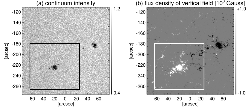
Figure 1: (a) Continuum intensity and (b) magnetic flux density of vertical field in NOAA AR 10972. The continuum intensity is normalized to the mean intensity of the quiet area outside the sunspots. These panels are made from observations with the Hinode SP from 15:05 to 15:37 on 2007 October 6. The box is identical to the field of view of Fig. 2. The positions in the vertical and horizontal axes are given with respect to the center of the solar disk.

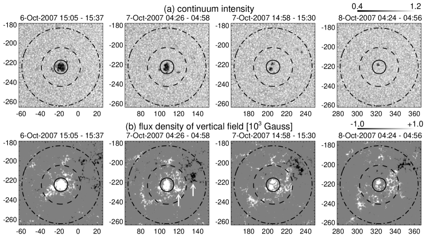
Figure 2: Time series of (a) continuum intensity and (b) magnetic flux density of vertical field for the following sunspot in NOAA AR 10972. The solid, dashed, and dash-dotted circles indicate the outer boundaries of regions called the sunspot region (7$\arcsec$ from the sunspot center), the unipolar region (20$\arcsec$ from the sunspot center), and the mixed polarity region (40$\arcsec$ from the sunspot center), respectively. The vertical and horizontal axes show the positions with respect to the disk center in units of arcseconds. The white arrows indicate an emerging bipole.

NOAA AR 10972 emerged on 2007 October 5 and formed a small bipolar sunspot, as shown in Figure 1. Both the leading and following sunspots completely disappeared at the end of October 8, leaving only plage regions. The Hinode SOT started to observe this active region from 14:00 on October 6, so that we did not observe the growing phase of the active region. However, SOT provided a good data set for the decay phase. We selected observations of the following sunspot from 15:05 on October 6 to 07:12 on October 8, at which time the sunspot had significantly decayed (Fig. 2). The reason why we focused on only the following sunspot was that a part of moat region surrounding the leading sunspot was outside the field of view. In this period, the spectropolarimeter (SP) of the SOT scanned the active region with the field of view of $152\arcsec\times 164\arcsec$ every 1-2 hr, except for two 4 hr gaps. This provided us a time series of spatial distributions of the full polarization state for two photospheric Fe I lines at 6301.5 Å and 6302.5 Å. The slit scanning step was 0.297$\arcsec$ with an integration time of 3.2 seconds (Fast mapping mode). SP took about 32 minutes to complete each scan. The pixel scale along the slit was 0.320$\arcsec$, which was binned 2 pixels with the original spatial resolution of SP. In the same period, the narrowband filter imager (NFI) of the SOT continously obtained Stokes I and V images of the active region at a wavelength of -172 mÅ from the center of the lower chromospheric Na D line at 5896 Å with a 2 minute cadence. The field of view was $276\arcsec\times 164\arcsec$ with a pixel sampling of 0.16$\arcsec$.

3 DATA ANALYSIS

3.1 Magnetic Flux Density

The temporal change of magnetic flux in and around the following sunspot was estimated from observations with the SP. The Stokes profiles of the two Fe lines were calibrated with a standard routine (“SP_-PREP”; B. W. Lites et al. 2008, in preparation). The magnetic field vector and thermodynamic parameters were derived from the calibrated Stokes profiles with a Milne-Eddington Stokes inversion (T. Yokoyama et al. 2008, in preparation). The inversion code provided us magnetic field vector in a line-of-sight frame. A two-component model atmosphere, in which the photospheric atmosphere was composed of a magnetized atmosphere (polarized light) and a non-magnetized atmosphere (non-polarized light), was assumed in the inversion code. We estimated a flux density of magnetic field vertical to the solar surface for the pixels that have the degree of polarization larger than 0.5 $\%$ as

$$F=\frac{1}{\cos\theta}f|{\bf{B}}|\cos\gamma,$$ (1)

where a heliocentric angle ($\theta$), field strength ($|{\bf{B}}|$), inclination angle ($\gamma$) with respect to the local vertical, and filling factor ($f$). The filling factor is an areal percentage of the magnetized atmosphere in each pixel.

A disambiguation of azimuth angles was needed to convert from the inclination with respect to the line-of-sight direction into the inclination with respect to the local vertical. To perform the disambiguation, we selected the azimuth angles closer to the azimuth of potential fields at the photospheric surface, and then interactively determined the azimuth to reduce discontinuities of azimuth and inclination angles by using the AZAM utility (written in IDL by P. Seagraves; Lites et al., 1995). The active region has a simple bipolar structure with simple unipolar spots. For such cases the ambiguity resolution with the AZAM is almost successfully performed (Metcalf et al., 2006). Furthermore, the sunspot was located near the disk center and the heliocentric angle ranges from 11$\arcdeg$ to 25$\arcdeg$. This means that projection effects of errors in magnetic field inclination due to the disambiguation of azimuth angle are small.

We applied an image cross-correlation for the magnetic flux density maps in order to align the SP maps obtained at different times. The area around the following sunspot was used in the image cross-correlation in order to accurately remove the proper motion of the following sunspot. We did not use continuum intensity maps in the image cross-correlation because magnetic features were still observed after the following sunspot became very small and the granulation patterns had changed significantly. This allows us to trace the change of magnetic flux until the disappearance of the sunspot.

3.2 Horizontal Velocity of Magnetic Elements

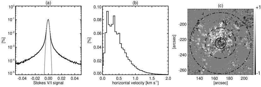
Figure 3: (a) Histogram of the magnetic signal in a line-of-sight NFI magnetogram (solid line). The gray line shows a result of a Gaussian fitted to a central part of the histogram. (b) Histogram of horizontal velocity calculated by the local correlation tracking technique that is applied for line-of-sight magnetograms. The horizontal velocities are averaged over the period taking each SP map (about 32 minutes). (c) Spatial distribution of a radial component of the horizontal velocity averaged over the period from 10:59:32 to 11:27:31 on 2007 October 7 in units of km s^-1. Positive corresponds to a radial outward motion. The circles are same as those in Fig. 2.

Horizontal velocities of magnetic elements are necessary for estimation of a flux transport rate. Hereafter, the Na D line-of-sight magnetogram is defined as the Stokes V image divided by the simultaneous Stokes I images. For each SP map (about 32 minutes), 16 line-of-sight magnetograms with a 2 minute cadence were obtained. We made 8 horizontal velocity maps with a 4 minute cadence from the 16 line-of-sight magnetograms, using a local correlation tracking method (LCT; November & Simon, 1988; Chae et al., 2001; Sakamoto, 2004). The apodization window was a Gaussian with the FWHM of 1$\arcsec$ in the LCT. The LCT was applied for the pixels that have Stokes V/I signals larger than 0.0015 in two sequential line-of-sight magnetograms. The threshold of 0.0015 was about 1$\sigma$ noise of the line-of-sight magnetograms. We assumed that the 1$\sigma$ noise of the line-of-sight magnetograms corresponds to the width parameter (the standard deviation) of a Gaussian fitted to a central part of a histogram for the signals in the line-of-sight magnetogram (Fig. 3a). When a pixel had a coss-correlation coefficient less than 0.9 or the Stokes V/I signal less than 0.0015, the horizontal velocity for the pixel was assumed to be 0 km s^-1.

Finally, we averaged over the 8 horizontal velocity maps, and then aligned the averaged map to the SP map obtained at the same period, using the image cross-correlation between the line-of-sight magnetic flux density with the SP and the line-of-sight magnetogram with the NFI. Figure 3b shows a histogram of the horizontal velocity. The average of the horizontal velocity is 0.5 km s^-1, which is similar to the averaged speed of MMFs and moat flow in previous studies (e.g. Brickhouse & Labonte, 1988; Zhang et al., 2003). Magnetic elements that move faster than the averaged moat flow of 0.5-1.0 km s^-1 (Hagenaar & Shine, 2005) are also detected. Furthermore, radial outward motions of magnetic elements can be seen around the following sunspot in Figure 3c. Thus, radial outward motions of MMFs are successfully obtained with the LCT.

4 RESULTS

Many moving magnetic features (MMFs) are observed outside the sunspot (Fig. 2b). The MMFs of positive polarity (the polarity of the following sunspot) are dominant in the region with a radial distance ($r_{s}$) less than 20$\arcsec$ from the center of the following sunspot. MMFs of both polarities are located in the region $r_{s}>20\arcsec$. Most magnetic elements with negative polarity are located in the north-western side to the sunspot, and are in contact with positive polarity elements. Hereafter, we call regions with $r_{s}=0\arcsec-7\arcsec$, $r_{s}=7\arcsec-20\arcsec$, and $r_{s}=20\arcsec-40\arcsec$ as the sunspot region, the unipolar region, and the mixed polarity region, respectively. In regular decaying sunspots, the unipolar region corresponds to the inner and middle moat region, and the mixed polarity region corresponds to the region around the outer boundary of the moat region. We investigate the temporal change of magnetic flux in these three regions, and also investigate how much magnetic flux passes the outer boundaries of the three regions.

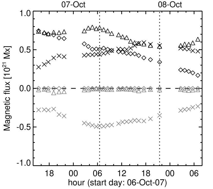
Figure 4: Time profiles of total magnetic flux in the sunspot region (diamond), unipolar region (triangle), and mixed polarity region (cross) as determined from the SP maps. The black symbols show magnetic flux of positive polarity, and the gray symbols show magnetic flux of negative polarity. The time profiles in the period between the two dotted lines are used for calculation of the flux change rate ($dF/dt$) in Fig. 5.

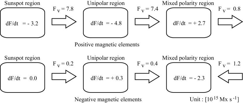
Figure 5: Summary of observations for the flux change rate ($dF/dt$) and the flux transport rate ($F_{v}$) in units of $10^{15}$Mx s^-1.

Positive magnetic flux decreases at a constant rate in the sunspot region, as shown in Figure 4. In the unipolar region, the positive magnetic flux increases from 01:00 to 06:00 on October 7 as a result of the flux emergence indicated by the arrows in Figure 2. The emerging bipoles appear close to $r_{s}=20\arcsec$ and the opposite polarities associated with the emergence separate in the the regions $r_{s}<20\arcsec$ ($r_{s}>20\arcsec$) for positive (negative) flux. This flux emergence also causes increase of the negative magnetic flux in the mixed polarity region. After the flux emergence, the positive flux in the unipolar region and the negative flux in the mixed polarity region decrease at similar rates. On the other hand, the positive flux in the mixed polarity region increases during this period. The negative magnetic flux in the sunspot and unipolar regions is much smaller than the signed fluxes in the other regions. We estimate an increase and decrease rate of magnetic flux in each region by a linear fit to the time profiles from 06:15 to 21:26 on October 7 in Figure 4. The magnetic flux changes nearly linearly during this period. The result is shown as “$dF/dt$” in Figure 5. Even when the sunspot becomes too small on October 8, the positive flux in the sunspot region still decreases at a constant rate. On the other hand, the positive flux does not show any increases and decreases in the unipolar region and mixed polarity region on October 8. This tendency already may be seen in the later part on October 7. The change of the tendency suggests the possibility of different flux loss process in remnant active regions, but further, more detailed, investigations of this phenomena are needed.

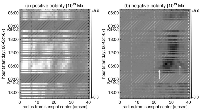
Figure 6: Total magnetic flux at each radius from the sunspot center vs. time for (a) positive polarity and (b) negative polarity . The total magnetic flux with positive (negative) polarity represents the sum total of magnetic flux for positive (negative) magnetic elements that have the same radius from the sunspot center. The hatched areas with oblique lines represent the periods without any SP observations. The dashed, dash-dotted, and dotted lines show the outer boundaries of the sunspot region (7$\arcsec$ from the sunspot center), the unipolar region (20$\arcsec$ from the sunspot center), and the mixed polarity region (40$\arcsec$ from the sunspot center), respectively.

Figure 6 shows temporal evolution of total magnetic flux at each radius from the sunspot center. The areas that have large positive magnetic flux move away from the sunspot toward the mixed polarity region. Such outward motion of the positive flux is due to magnetic flux transported by the MMFs of positive polarity. The outward motion of the positive flux stops around 30$\arcsec$ from the sunspot center. Figure 2 also shows that most of the positive magnetic elements do not go out of the mixed polarity region, except for the positive elements located in the north-eastern side to the sunspot. Most of the negative magnetic flux is located around 30$\arcsec$ from the sunspot center, and converging motion of the negative flux is observed around the 30$\arcsec$ from the sunspot center (indicated by the arrows in Fig. 6). These results suggest that the boundary of a supergranular cell, which corresponds to the outer boundary of the moat region, is located around 30$\arcsec$ from the sunspot center.

We estimate a radial transport rate ($F_{v}(r_{s})$) of magnetic flux at each radius ($r_{s}$) from the sunspot center using the following formula:

$$F_{v}(r_{s})={\sum_{r_{s}=r_{1}}^{r_{2}}}\frac{|F(r_{s})|}{\pi(r_{2}^{2}-r_{1}^{2})}v_{r}(r_{s})\frac{2\pi(r_{1}+r_{2})}{2},$$ (2)

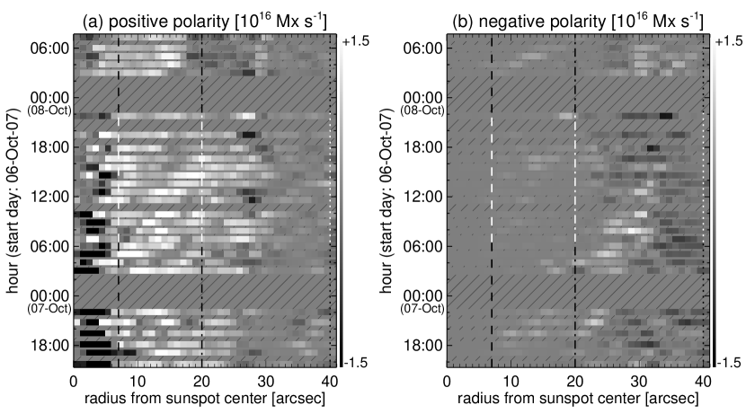
Figure 7: Same as Fig. 6, but for showing the flux transport rate vs. time. The flux transport rate ($F_{v}(r_{s})$) is calculated as Eq. (2). The white indicates magnetic flux transported away from the sunspot center. The value averaged along the white part of each line is identical to the flux transport rate ($F_{v}$) in Fig. 5.

where $F(r_{s})$ is the magnetic flux density of vertical fields (Eq. (1)) and $v_{r}(r_{s})$ is the radial component of horizontal velocity at $r_{s}$. We set $r_{1}$ and $r_{2}$ as $r_{s}\pm 1\arcsec$, respectively. The behavior of $F_{v}(r_{s})$ with time in Figure 7 shows that the motions of magnetic flux seen in Figure 6 (e.g. outward motion of the positive flux, converging motion of the negative flux) are obtained by using Equation (2). The inward flux transport rate for positive polarity elements around the sunspot center is probably incorrect. This anomaly is mainly due to the shrinkage of the sunspot, yielding spurious inward $v_{r}(r_{s})$: the LCT does not work well when the contrast of line-of-sight magnetograms is low. However, the flux transport within the sunspot region is not the object of this study. We focus on the flux transport rates at the outer edges of the sunspot region as well as the unipolar and mixed polarity regions during the period when the flux change rate is calculated from Figure 4 (06:15 to 21:26 on October 7). The flux transport rates averaged over this period are summarized as “$F_{v}$” in Figure 5. The direction of the arrows shows whether magnetic flux is transported radially inward or outward.

5 DISCUSSION AND CONCLUSIONS

The averaged flux change and averaged flux transport in Figure 5 are described in units of Mx s^-1, so that we can compare these values directly. The observed flux change [$(dF/dt)_{Obs}$] in each region and the observed flux transport [$(F_{v})_{Obs}$] at its boundaries would have a relationship:

$$(\frac{dF}{dt})_{Obs}=(\frac{dF}{dt})_{Emerge}-(\frac{dF}{dt})_{Loss}\pm(F_{v})_{Obs}.$$ (3)

The increase of magnetic flux due to flux emergence [$(dF/dt)_{Emerge}$] can be neglected in this case, because we select the period without any significant flux emergence. Thus, we can estimate an actual flux loss rate [$(dF/dt)_{Loss}$] in each region from the observations.

The total of flux decrease rates in the sunspot and unipolar regions ($dF/dt$ = -3.2 - 4.8 = -8.0$\times 10^{15}$ Mx s^-1) is almost equal to the flux transport rate at the outer boundary of the unipolar region for the positive polarity ($F_{v}$ = 7.4$\times 10^{15}$ Mx s^-1). This means that most of magnetic flux that disappeared in the sunspot and unipolar regions is carried away to the mixed polarity region. Note that we do not trace each magnetic element, and all of the MMFs that separated from the sunspot may not reach at the outer boundary of the unipolar region. However, we make Figure 5 from the observations for about 12 hr, which is twice as long as the period that magnetic elements with the average horizontal speed of 0.5 km s^-1 need to move through the unipolar region of a width of 14$\arcsec$. The increase of the positive flux in the mixed polarity region supports the migration of positive flux into the mixed polarity region. Both the increase of the positive flux in the mixed polarity region and the flux transport for the positive polarity elements at the outer boundary of the mixed polarity region are smaller than the positive flux transported from the unipolar region. Therefore, the magnetic flux that is carried away from the sunspot (and moat region) mostly disappears in the mixed polarity region, especially near the outer boundary of the moat region.

One issue is that the positive flux carried away from the sunspot region ($F_{v}$ = 7.8$\times 10^{15}$ Mx s^-1) is bigger than decrease of the positive flux in the sunspot region ($dF/dt$ = -3.2$\times 10^{15}$ Mx s^-1). This tendency was also reported in the previous work with a lower (about $1\arcsec$) spatial resolution (Kubo et al., 2007). As a result of no flux emergence in the sunspot region, the flux transport rate should be less than the flux decrease rate in the sunspot region. That is to say that the flux transport rate is overestimated at the outer boundary of the sunspot region. In the calculation of horizontal velocities, we use the apodization window with 1$\arcsec$, which is lower than the spatial resolution of the magnetic field maps. Such a lower spatial resolution of the horizontal velocity maps probably causes the overestimation of the flux transport rate at the outer boundary of the sunspot region. Fuzzy, small magnetic elements with a short lifetime have been observed around the outer boundary of decaying sunspots (Zhang et al., 2007; Kubo et al., 2008). These fuzzy magnetic elements have higher outward motion and smaller magnetic flux than those of usual MMFs. In the estimation of flux transport at the outer boundary of the sunspot, magnetic flux is mostly represented by MMFs with small horizontal velocity and large magnetic flux, but its horizontal velocity is represented by the fuzzy magnetic elements. We believe that these fuzzy magnetic elements correspond to a fluctuation of field strength or a fluctuation of inclination of penumbral magnetic fields, and thus do not contribute to the flux loss of the sunspot. Further investigation using spectropolarimetric measurements with a higher cadence will be necessary to know the nature of such fuzzy magnetic elements and their impact on the presented calculations.

The magnetic flux of negative polarity decreases in the mixed polarity region, although the negative flux converges from the inner and outer boundaries of the mixed polarity region. Considering that the negative flux moves into the mixed polarity region with the average rate of 1.6$\times 10^{15}$ Mx s^-1, the actual flux loss rate [$(dF/dt)_{Loss}$] in the mixed polarity region may be as large as 3.9$\times 10^{15}$ Mx s^-1 from Equation (3). This flux loss rate of negative polarity is balanced by the actual flux loss rate of the positive polarity (3.9$\times 10^{15}$ Mx s^-1), which is a difference between the flux transport rate ($F_{v}$ = 7.4 - 0.8 = 6.6$\times 10^{15}$ Mx s^-1) into the mixed polarity region and the flux increase rate ($dF/dt$ = 2.7$\times 10^{15}$ Mx s^-1) there. The flux loss rates with both polarities in the mixed polarity region are consistent with the cancellation rates in active regions (Chae et al., 2000, 2004; Kubo & Shimizu, 2007). Furthermore, most of the magnetic elements with negative polarity are located in contact with the positive elements. These results suggest that magnetic flux cancellation at the outer boundary of the moat region is essential for the removal of the sunspot magnetic flux from the photosphere.

References

- Bellot Rubio & Beck (2005) Bellot Rubio, L. R., & Beck, C. 2005, ApJ, 626, L125
- Bray & Loughhead (1964) Bray, R. J., & Loughhead, R. E. 1964, The International Astrophysics Series, London: Chapman Hall, 1964,
- Brickhouse & Labonte (1988) Brickhouse, N. S. & Labonte, B. J. 1988, Sol. Phys., 115, 43
- Chae et al. (2000) Chae, J., Denker, C., Spirock, T. J., Wang, H., & Goode, P. R. 2000, Sol. Phys., 195, 333
- Chae et al. (2001) Chae, J., Martin, S. F., Yun, H. S., Kim, J., Lee, S., Goode, P. R., Spirock, T., & Wang, H. 2001, ApJ, 548, 497
- Chae et al. (2004) Chae, J., Moon, Y., & Pevtsov, A. A. 2004, ApJ, 602, L65
- Hagenaar & Shine (2005) Hagenaar, H. J., & Shine, R. A. 2005, ApJ, 635, 659
- Harvey & Harvey (1973) Harvey, K. & Harvey, J. 1973, Sol. Phys., 28, 61
- Harvey et al. (1999) Harvey, K. L., Jones, H. P., Schrijver, C. J., & Penn, M. J. 1999, Sol. Phys., 190, 35
- Lites et al. (1995) Lites, B. W., Low, B. C., Martinez Pillet, V., Seagraves, P., Skumanich, A., Frank, Z. A., Shine, R. A., & Tsuneta, S. 1995, ApJ, 446, 877
- Martin, Livi, & Wang (1985) Martin, S. F., Livi, S. H. B., & Wang, J. 1985, Australian Journal of Physics, 38, 929
- Martínez Pillet (2002) Martínez Pillet, V. 2002, Astronomische Nachrichten, 323, 342
- Metcalf et al. (2006) Metcalf, T. R., et al. 2006, Sol. Phys., 237, 267
- November & Simon (1988) November, L. J. & Simon, G. W. 1988, ApJ, 333, 427
- Kosugi et al. (2007) Kosugi, T., et al. 2007, Sol. Phys., 243, 3
- Kubo et al. (2007) Kubo, M., Shimizu, T., & Tsuneta, S. 2007, ApJ, 659, 812
- Kubo & Shimizu (2007) Kubo, M., & Shimizu, T. 2007, ApJ, 671, 990
- Kubo et al. (2008) Kubo, M., et al. 2008, ApJ, 681, 1677
- Sakamoto (2004) Sakamoto, Y. 2004, ASP Conf. Ser. 325: The Solar-B Mission and the Forefront of Solar Physics, 325, 151
- Tsuneta et al. (2008) Tsuneta, S., et al. 2008, Sol. Phys., 249, 167
- Wang et al. (1991) Wang, H., Zirin, H., & Ai, G. 1991, Sol. Phys., 131, 53
- Wang & Shi (1993) Wang, J. & Shi, Z. 1993, Sol. Phys., 143, 119
- Yurchyshyn & Wang (2001) Yurchyshyn, V. B. & Wang, H. 2001, Sol. Phys., 202, 309
- Zhang et al. (2003) Zhang, J., Solanki, S. K., & Wang, J. 2003, A&A, 399, 755
- Zhang et al. (2007) Zhang, J., Solanki, S. K., & Woch, J. 2007, A&A, 475, 695
- Zwaan (1987) Zwaan, C. 1987, ARA&A, 25, 83