On the Difference in Statistical Behavior Between Astrometric and Radial-Velocity Planet Detections

Abstract

Astrometric and radial-velocity planet detections track very similar motions, and one generally expects that the statistical properties of the detections would also be similar after they are scaled to the signal-to-noise ratio of the underlying observations. I show that this expectation is realized for periods small compared to the duration of the experiment $P/T\ll 1$, but not when $P/T\gtrsim 1$. At longer periods, the fact that models of astrometric observations must take account of an extra nuisance parameter causes the mass error to begin deteriorating at $P/T\sim 0.8$, as compared to $P/T\sim 1.0$ for RV. Moreover, the deterioration is much less graceful. This qualitative difference carries over to the more complicated case in which the planet is being monitored in the presence of a distant companion that generates an approximately uniform acceleration. The period errors begin deteriorating somewhat earlier in all cases, but the situation is qualitatively similar to that of the mass errors. These results imply that to preserve astrometric discovery space at the longest accessible orbits (which nominally have the lowest-mass sensitivity) requires supplementary observations to identify or rule out distant companions that could contribute quasi-uniform acceleration.

1 Introduction

Astrometric and radial-velocity (RV) planet detections are, from a mathematical standpoint, extremely similar. In each, one models 1-dimensional projections of Kepler orbits and attempts to fit Kepler parameters. In the limit of circular orbits, the planet signature is encoded in the simple form

$$F(t;a_{1},a_{2},a_{3})=a_{1}\sin(a_{2}t+a_{3}),$$ (1)

where

$$a_{1}=\alpha\quad{\rm(astrometry)},\qquad a_{1}=K\quad{\rm(RV)},$$ (2)

are the astrometric and velocity semi-amplitudes for the two cases, and where

$$a_{2}={2\pi\over P},\quad a_{3}=\phi\qquad{\rm(astrometry+RV)}$$ (3)

designate the period $P$ and phase $\phi$, respectively. One then goes on to combine information about the star’s mass and (for astrometry) its distance, to infer the planet mass $m$ (astrometry) or $m\sin i$ (RV), where $i$ is the inclination. In the astrometric case, there are of course two such equations, one for each direction in the plane of the sky, whose ratio gives $\cos i$, and so permit one to break the $m\sin i$ degeneracy that plagues the intrinsically 1-dimensional RV measurement.

Because the form of equation (1) is essentially identical in the two cases, it is generally assumed that the error properties, i.e., the relation between the measurement errors and the derived-parameter errors, is also the same. Of course, it is well known that the parameter errors have a different dependence on semimajor axis $a$, system distance $D$, etc. Most notably, with other parameters held fixed, astrometric sensitivity increases linearly with $a$ whereas RV sensitivity declines as $a^{-1/2}$. But here I am referring to something else. The differences just mentioned all impact the final result because they change the characteristic signal-to-noise ratio of the experiment,

$${\rm SNR}\equiv{a_{1}\over\sigma}\sqrt{N},$$ (4)

where $N$ is the number of measurements and $\sigma$ is the error in each measurement (assumed for simplicity to be all the same). Here I will show that the astrometric and RV measurements have substantially different error properties even when SNR is identical.

2 Minimum Variance Bound

I will work within the framework of the minimum variance bound (MVB), also frequently called the Fisher-matrix approximation. As the same approximation will be applied to both techniques, this will allow me to highlight the difference between them. Of course, if equation (1) really did fully represent both techniques, there could not be any difference in their error properties. However, the true functional forms of the source motions are actually

$$F(t;a_{i})=a_{1}\sin(a_{2}t+a_{3})+\sum_{i=4}^{n}a_{i}t^{i-4}.$$ (5)

For simplicity, I will continue to assume circular orbits, and I will assume for the astrometric case that the orbit is seen edge-on. In fact, the latter is not much of an approximation since in most cases the great majority of the information about the mass and period comes from the major axis of the apparent astrometric ellipse. Finally, I will assume that the data are taken uniformly in time, at intervals that are frequent compared to the orbital period, and that they all have the same error, $\sigma$.

For a single-planet, i.e., a system composed of just a star and a planet, in which the star does not suffer any other accelerations, $n=4$ for the RV case, but $n=5$ for the astrometric case. For RV, $a_{4}$ is the systemic radial velocity of the system. For astrometry, $a_{5}$ is the systemic proper motion of the system, while $a_{4}$ is the zero point of that motion.

The introduction of the nuisances parameters $a_{4}$ or $(a_{4},a_{5})$ is what distinguishes the two cases statistically. The difference appears only for $P\sim T$ or $P>T$, where $T$ is the duration of the experiment. I have implicitly assumed that $T,P\gg 1\,\rm yr$, and this is the reason that I ignore parallax, which would be an additional nuisance parameter for astrometry, but not for RV.

In the Fisher-matrix approximation, the inverse covariance matrix of the parameters, $b_{ij}$, is given by

$$b_{ij}\equiv\sum_{k}{f_{i}(t_{k})f_{j}(t_{k})\over\sigma_{k}^{2}}\rightarrow{N\over\sigma^{2}}\,{1\over T}\int_{0}^{T}dtf_{i}(t)f_{j}(t)$$ (6)

where

$$f_{i}(t)\equiv{\partial F(t)\over\partial a_{i}}.$$ (7)

One easily finds that for $P\ll T$, $a_{1}$ and $a_{2}$ are completely uncorrelated from the other parameters, so that

$${\sigma(a_{1})\over a_{1}}\equiv{\sqrt{c_{11}}\over a_{1}}\rightarrow{1\over\sqrt{b_{11}}a_{1}}=\sqrt{2\over N}\,{\sigma\over a_{1}}={\sqrt{2}\over\rm SNR}.$$ (8)

That is, $\sigma(a_{1})/a_{1}$, which is the fractional error in astrometric or RV amplitude depends only on SNR, and in a very simple way. Similarly,

$${\sigma(P)\over P}={\sigma(a_{2})\over a_{2}}\rightarrow{1\over\sqrt{b_{22}}a_{2}}={\sqrt{6}/\pi\over\rm SNR}\,{P\over T}.$$ (9)

However, as $P$ approaches $T$, the parameters of primary interest (mass and period) become correlated with the nuisance parameters. To calculate this effect, I employ equations (6) and (7), but using the full 7-parameter Kepler formalism, not just the three Kepler parameters displayed in equations (1) and (5). That is, even though the adopted orbits are circular and edge-on, I allow for free fits to the eccentricity and inclination, and so for correlations between these parameters (as well as the two remaining Kepler parameters) and the parameters of interest (amplitude and period). The effect of allowing for these covariances is to increase the errors in semi-amplitude and period by modest amounts relative to what would be obtained using equation (5).

Panels (a) and (b) of Figure 1 show the ratios of the true errors for the amplitude and period, respectively, relative to the naive equations (8) and (9), for both the RV (green) and astrometric (red) cases. In fact, as I will discuss in § 4, for $P\gtrsim T$, the errors depends on phase as well as period. Figure 1 therefore shows the root-mean-square of the errors, averaged over all phases. Note that the RV amplitude errors follow the naive form until $P/T\sim 1.1$ and then deteriorate relatively gracefully. By contrast, the astrometric errors begin deviating at $P/T\sim 0.75$ and then deteriorate much more quickly. For the period errors, deterioration begins at $P/T\sim 0.85$ for RV and $P/T\sim 0.65$ for astrometry, but the overall pattern is qualitatively similar.

The mass estimates for astrometry and RV depend on different combinations of amplitude and period,

$$m\propto a_{1}a_{2}^{n}\qquad\biggl{(}n={2\over 3}\quad{\rm Ast};\quad n=-{1\over 3}\quad{\rm RV}\biggr{)}$$ (10)

Hence the fractional error in the mass (or $m\sin i$ in the case of RV) is related to the errors in the fit parameters by

$$\biggl{[}{\sigma(m)\over m}\biggl{]}^{2}={c_{11}\over a_{1}^{2}}+2n{c_{12}\over a_{1}a_{2}}+n^{2}{c_{22}\over a_{2}^{2}}.$$ (11)

In the limit $P\ll T$, $\sigma(m)/m\rightarrow\sigma(a_{1})/a_{1}$, but for $P\gtrsim T$, the period error and the correlations become important. Figure 1c shows the results of calculations that apply equation (11).

3 Additional Uniform Acceleration

Of course, the star may have more than one companion (planetary or otherwise), and one may imagine arbitrarily complicated configurations. Here I restrict myself to the next level of complication, a second companion that is sufficiently far away that its effect on the star may be treated as uniform acceleration. Even if no such acceleration is identified, one might decide to fit for it on the grounds that there may be such a companion that has not been recognized. I now ask how the inclusion of such an additional nuisance parameter affects the precision of the physical parameters for the planet that was previously treated as isolated.

The number of nuisance parameters is incremented by one in each case. Referring to equation (5), for RV, we now have $n=5$, with $a_{5}$ being the systemic acceleration, while for astrometry, $n=6$, with $a_{6}$ being the systemic proper-motion acceleration. Figures 1a and 1b show the corresponding ratios relative to the naive equations (8) and (9). In this case, RV is represented by the red curve, while astrometry is represented by the blue curve. The fractional mass errors are shown by solid curves in Figure 1c.

In this case, both deteriorate rapidly, but the mass-error deterioration begins at $P/T\sim 0.65$ for astrometry and at $P/T\sim 0.75$ for RV. One may anticipate that in other, yet more complicated situations, RV will always perform like the naive equations to higher $P/T$ than astrometry, simply because it has one fewer nuisance parameter.

4 Phase Dependence

Figure 1 shows the root-mean-square errors averaged over phase. In fact, as $P/T$ grows and the rms errors deteriorate, the variations with phase also increase. Figure 2 shows the phase variations of the mass errors for the particular case that the period is exactly equal to the duration of the experiment, $P/T=1$. These large variations imply that Figure 1 cannot be used to estimate the errors in any particular case (except if the rms ratio is close to unity). Rather, it should be used as a general guide to the reliability of the experiment. Any individual planet detection must be analyzed based on the actual data and the parameters derived.

5 Discussion

The results derived here are primarily of interest in regard to future astrometric missions such as GAIA and SIM. The first point is that planets with periods that are even slightly longer than the mission cannot be reliably detected unless they are many times more massive than the nominal thresholds of detection. And second, if one is forced to allow for uniform acceleration, then the same statement applies to $P/T\gtrsim 0.7$. Hence, to preserve the discovery space at the longest accessible periods, it is critically important to identify or rule out distant perturbers by supplementary data, such as longer-term RV observations to look for large, distant planetary or stellar companions, or perhaps AO observations to find stellar companions. This should be relatively straightforward for SIM, with its limited number of high-precision targets, but may be more difficult for GAIA, which is a survey instrument.

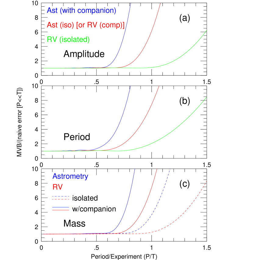
Figure 1: Panels (a) and (b): ratios of true amplitude and period error to naive eqs. (8) and (9) as a function of $P/T$ and averaged over all phases $\phi$. Case of star with single planet is shown for RV (green curve) and astrometry (red curve). They differ because astrometry has one extra nuisance parameter (proper motion). If the star suffers an extra source of uniform acceleration from another companion, there is an additional nuisance parameter for both RV (red curve) and astrometry (blue curve). In all cases, RV follows the naive equation to higher $P/T$ and degrades thereafter more gracefully. Panel (c): same ratio for the mass error relative to eq. (8). Both the isolated (dashed curves) and uniform-acceleration (solid curves) cases are shown for RV (blue curves) and astrometry (red curves). Note that the isolated-planet astrometry curve is no longer identical to the uniformly-accelerated RV curve, as was true for amplitude and period. This is because the mass is derived from different combinations of the amplitude and period for the astrometric and RV cases (eqs. [10-11]).

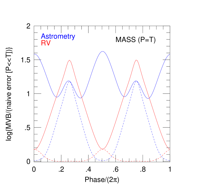
Figure 2: Ratio of the true mass error to that given by the naive eq. (8) as a function of phase $\phi$ for the special case $P/T=1$. When the ordinate in Fig. 1 is large, the variations with phase are also large. Hence, Fig. 1 should be regarded as a guide to the statistical properties of the experiments rather than a precise estimate of the errors in any particular planet detection.