A-graded methods for monomial ideals

Abstract.

We use ${\mathbb{Z}}^{d}$-gradings to study $d$-dimensional monomial ideals. The Koszul functor is employed to interpret the quasidegrees of local cohomology in terms of the geometry of distractions and to explicitly compute the multiplicities of exponents. These multigraded techniques originate from the study of hypergeometric systems of differential equations.

1. Introduction

A cornerstone of combinatorial commutative algebra is the connection between simplicial complexes and ideals generated by squarefree monomials, also known as Stanley–Reisner ideals. One of the fundamental results in this theory is Reisner’s criterion (Theorem 3.8), which expresses the Cohen–Macaulayness of a Stanley–Reisner ring as a topological condition on the corresponding simplicial complex.

These ideas can be adapted to study monomial ideals $I$ that are not squarefree. For instance, polarization produces a squarefree monomial ideal that shares many important properties with $I$. However, this construction introduces (many) new variables, making it impractical from a computational standpoint (see Example 3.17).

In contrast, the distraction of a monomial ideal $I$ (used in Hartshorne’s work on the Hilbert scheme [Har66]) has many of the features of its polarization, without the increase in dimension. While the distraction of $I$ is not a monomial ideal unless $I$ is squarefree, it can be studied using a finite family of simplicial complexes, called exponent complexes (see Definition 3.1).

Distractions arise naturally in the algebraic study of differential equations. Let $I$ be a monomial ideal in the ring ${\mathbb{C}}[\partial]={\mathbb{C}}[\partial_{1},\dots,\partial_{n}]$, a commutative polynomial subalgebra of the Weyl algebra $D_{n}$ of linear partial differential operators on ${\mathbb{C}}[x_{1},\dots,x_{n}]$, where $\partial_{i}$ denotes the operator ${\partial}/{\partial x_{i}}$. Let $\theta_{i}=x_{i}\partial_{i}$, so that ${\mathbb{C}}[\theta]={\mathbb{C}}[\theta_{1},\dots,\theta_{n}]$ is also a commutative polynomial subalgebra of $D_{n}$. The distraction of $I\subseteq{\mathbb{C}}[\partial]$ is the ideal

$$\tilde{I}=({\mathbb{C}}(x)\otimes_{{\mathbb{C}}[x]}D\cdot I)\cap{\mathbb{C}}[\theta]\subseteq{\mathbb{C}}[\theta].$$

Let $d=\dim({\mathbb{C}}[\partial]/I)$. Any integer matrix $A$ whose columns $a_{1},\dots,a_{n}$ span ${\mathbb{Z}}^{d}$ as a lattice induces a ${\mathbb{Z}}^{d}$-grading on $D_{n}$ via ${\rm tdeg}(\partial_{j})=a_{j}=-{\rm tdeg}(x_{j})$. Monomial ideals and their distractions are $A$-homogeneous and have the same holomorphic solutions when considered as systems of differential equations. While this solution space is usually infinite dimensional, its subspace of $A$-homogeneous solutions of any particular degree is finite dimensional (see Definition 2.9). One captures these solutions by adding Euler operators to these ideals, where a chosen degree is viewed as a parameter.

In this article we compute the dimension of the $A$-homogeneous holomorphic solutions of $I$ as a function of the parameters. Our starting point is Theorem 2.13, which provides a strong link between the Koszul homology of ${\mathbb{C}}[\theta]/\tilde{I}$ with respect to the Euler operators and the $A$-graded structure of the local cohomology of ${\mathbb{C}}[\partial]/I$ at the maximal ideal. The background necessary for this result occupies Section 2. In Section 3, we use the exponent complexes of $\tilde{I}$ to provide a new topological criterion for the Cohen–Macaulayness of the monomial ideal $I$, Theorem 3.12. Finally, in Section 4, we give a combinatorial formula for the dimension of the $A$-homogeneous holomorphic solutions of $I$ of a fixed degree, which may be viewed as an intersection multiplicity (see Theorem 4.5 and Proposition 4.1).

This work was inspired by the theory of $A$-hypergeometric differential equations, whose intuition and techniques are employed throughout, especially those developed in [SST00, MMW05, DMM06, Ber08]. As we apply results from partial differential equations in Sections 2 and 3, we use the ground field ${\mathbb{C}}$. Our techniques in Section 4 are entirely homological and thus work over any field of characteristic zero. Since our findings were first circulated, Ezra Miller [Mil08] has found alternative commutative algebra proofs for the results in Section 3, as well as a version of Theorem 2.13, which are valid over an arbitrary field.

Acknowledgments

We are grateful to Uli Walther for his hospitality while the second author visited Purdue University, and for thoughtful comments that improved a previous version of this article. We also thank Giulio Caviglia, who pointed us to the polarization of monomial ideals, Vic Reiner, for crucial advice on simplicial matroids that benefited Section 4, and Bernd Sturmfels, for his encouraging comments. We especially thank Ezra Miller, who made us aware of important references, and offered many valuable suggestions, including the clarification of Remark 3.2.

2. Differential operators, local cohomology, and ${\mathbb{Z}}^{d}$-gradings

Although our results can be stated in commutative terms, our methods and ideas come from the study of hypergeometric differential equations. Thus, we start by introducing the Weyl algebra $D=D_{n}$ of linear partial differential operators with polynomial coefficients:

$$D={\mathbb{C}}\left\langle x,\partial\;\bigg{|}\;[\partial_{i},x_{j}]=\delta_{ij},[x_{i},x_{j}]=0=[\partial_{i},\partial_{j}]\right\rangle,$$

where $x=x_{1},\dots,x_{n}$ and $\partial=\partial_{1},\dots,\partial_{n}$. We distinguish two commutative polynomial subrings of $D$, namely ${\mathbb{C}}[\partial]={\mathbb{C}}[\partial_{1},\dots,\partial_{n}]$ and ${\mathbb{C}}[\theta]={\mathbb{C}}[\theta_{1},\dots,\theta_{n}]$, where the $\theta_{i}=x_{i}\partial_{i}$, and we denote ${\mathfrak{m}}=\langle\partial_{1},\dots,\partial_{n}\rangle\subseteq{\mathbb{C}}[\partial]$.

Convention 2.1.

Henceforth, $I$ is a monomial ideal in ${\mathbb{C}}[\partial]$, and $d$ denotes the Krull dimension of the ring ${\mathbb{C}}[\partial]/I$.

Definition 2.2.

Given any left $D$-ideal $J$, the distraction of $J$ is the ideal

$$\tilde{J}=({\mathbb{C}}(x)\otimes_{{\mathbb{C}}[x]}D\cdot J)\cap{\mathbb{C}}[\theta]\subseteq{\mathbb{C}}[\theta].$$

For the monomial ideal $I\subseteq{\mathbb{C}}[\partial]$, the identity $x_{i}^{m}\partial_{i}^{m}=\theta_{i}(\theta_{i}-1)\cdots(\theta_{i}-m+1)$ implies that

(2.1) $$\tilde{I}={\widetilde{(D\cdot I)}}=\left\langle[\theta]_{u}:=\prod_{i=1}^{n}\prod_{j=0}^{u_{i}-1}(\theta_{i}-j)\ \bigg{|}\ \partial^{u}\in I\right\rangle.$$

Remark 2.3.

We emphasize that $I$ and $\tilde{I}$ live in different $n$-dimensional polynomial rings. Also, note that the zero set of the distraction $\tilde{I}$ is the Zariski closure in ${\mathbb{C}}^{n}$ of the exponent vectors of the standard monomials of $I$.

Remark 2.4.

We can think of $I$ and $\tilde{I}$ either as systems of partial differential equations or as systems of polynomial equations, and this dichotomy will be useful later on. To avoid confusion, a solution of $I$ or $\tilde{I}$ will always be a holomorphic function, while the name zero set (and the notation ${\mathbb{V}}(I)$, ${\mathbb{V}}(\tilde{I})$) is reserved for an algebraic variety in ${\mathbb{C}}^{n}$.

A monomial ideal in ${\mathbb{C}}[\partial]$ is automatically homogeneous with respect to every natural grading of the polynomial ring, from the usual (coarse) ${\mathbb{Z}}$-grading to the finest grading by ${\mathbb{N}}^{n}$. In this article we take the middle road and use a ${\mathbb{Z}}^{d}$-grading, where $d=\dim({\mathbb{C}}[\partial]/I)$.

Definition 2.5.

A ${\mathbb{Z}}^{d}$-grading, called an $A$-grading, of the Weyl algebra $D$ is determined by a matrix $A\in{\mathbb{Z}}^{d\times n}$, or more precisely by its columns $a_{1},\dots,a_{n}\in{\mathbb{Z}}^{d}$ via

$${\rm tdeg}(x_{i})=-a_{i},\quad{\rm tdeg}(\partial_{i})=a_{i}$$

Given an $A$-graded $D$-module $M$, the set of true degrees of $M$ is

$${\rm tdeg}(M)=\{\alpha\in{\mathbb{Z}}^{d}\mid M_{\alpha}\neq 0\}\subseteq{\mathbb{Z}}^{d}.$$

The set of quasidegrees of $M$, denoted by ${\rm qdeg}(M)$, is the Zariski closure of ${\rm tdeg}(M)$ under the natural inclusion ${\mathbb{Z}}^{d}\subseteq{\mathbb{C}}^{d}$.

The notions of ${\rm tdeg}$ and ${\rm qdeg}$ arise from the $A$-grading of $D$, and should not be confused with the degree $\deg$ of a homogeneous ideal in a polynomial ring that is computed using the Hilbert polynomial, as in the following definition.

Definition 2.6.

The Hilbert polynomial of ${\mathbb{C}}[\partial]/I$ (with respect to the standard ${\mathbb{Z}}$-grading on ${\mathbb{C}}[\partial]$) has the form $P_{I}(z)=\frac{m}{d!}z^{d}+\cdots$. The degree of $I$, denoted by $\deg(I)$ is the number $m$, which is equal to the number of intersection points (counted with multiplicity) of ${\mathbb{V}}(I)$ and a sufficiently generic affine space of dimension $n-d$.

The local cohomology modules of ${\mathbb{C}}[\partial]/I$ with respect to the ideal ${\mathfrak{m}}=\langle\partial_{1},\dots,\partial_{n}\rangle$ are also $A$-graded. We describe the quasidegrees of $\bigoplus_{i<d}H^{i}_{{\mathfrak{m}}}({\mathbb{C}}[\partial]/I)$ in Theorem 2.13. First, we make precise the conditions required of our grading matrix $A$.

Convention 2.7.

Let $I\subseteq{\mathbb{C}}[\partial]$ be a monomial ideal of Krull dimension $d$. For the remainder of this article, we fix a $d\times n$ integer matrix $A$ such that

1. ${\mathbb{Z}}A={\mathbb{Z}}^{d}$,

2. ${\mathbb{N}}A\cap(-{\mathbb{N}}A)=0$,

3. For each $\sigma\subseteq\{1,\dots,n\}$, $\dim_{{\mathbb{Q}}}({\rm Span}\{a_{i}\mid i\in\sigma\})=\min(d,|\sigma|)$, where $|\sigma|$ is the cardinality of $\sigma$.

Notation 2.8.

We denote by $E_{i}$ the linear form $\sum_{j=1}^{n}a_{ij}\theta_{j}\in{\mathbb{C}}[\theta]$, where $A=(a_{ij})$ is our matrix from Convention 2.7. For $\beta\in{\mathbb{C}}^{d}$, let $E-\beta$ denote the sequence $\{E_{i}-\beta_{i}\}_{i=1}^{d}$ of Euler operators; in particular, $E$ is the sequence $E_{1},\dots,E_{d}$.

In Convention 2.7, the first condition ensures that our grading group is all of ${\mathbb{Z}}^{d}$, the second that the cone spanned by the columns of $A$ is pointed, that is, contains no lines. The third condition is used in the computations in Section 4, and implies that ${\mathbb{C}}[\theta]/(\tilde{I}+\langle E-\beta\rangle)$ is Artinian for all $\beta\in{\mathbb{C}}^{d}$. Further, it implies that the sequence of polynomials given by the coordinates of $A\cdot\partial$, for $\partial$ the column vector $[\partial_{1},\dots,\partial_{n}]^{t}$, is a linear system of parameters for $I$. A generic $d\times n$ integral matrix will satisfy these requirements.

Given a $d$-dimensional monomial ideal $I\subseteq{\mathbb{C}}[\partial]$ as in Convention 2.1, a matrix $A$ as in Convention 2.7, and a parameter vector $\beta\in{\mathbb{C}}^{d}$, our main object of study is the left $D$-ideal

$$I+\langle E-\beta\rangle\subseteq D.$$

As with all left $D$-ideals, $I+\langle E-\beta\rangle$ is a system of partial differential equations, so we may consider its space of germs of holomorphic solutions at a generic nonsingular point in ${\mathbb{C}}^{n}$.

Definition 2.9.

By the choice of $A$ in Convention 2.7, $I+\langle E-\beta\rangle$ is holonomic (see [SST00, Definition 1.4.8]), so the dimension of this solution space, called the holonomic rank of the system and denoted ${\rm rank\ }(I+\langle E-\beta\rangle)$, is finite.

If $\phi(x)$ is a solution of $I+\langle E-\beta\rangle$ and $t\in({\mathbb{C}}^{*})^{d}$, then $\phi(t^{a_{1}}x_{1},\dots,t^{a_{n}}x_{n})=t^{\beta}\phi(x)$. This justifies the claim in the Introduction: ${\rm rank\ }(I+\langle E-\beta\rangle)$ is the dimension of the space of holomorphic solutions of $I$ that are $A$-homogeneous of degree $\beta$.

Lemma 2.10.

Let $I\subseteq{\mathbb{C}}[\partial]$ be a monomial ideal and $\tilde{I}\subseteq{\mathbb{C}}[\theta]$ its distraction. Then there is an equality of ranks: ${\rm rank\ }(I+\langle E-\beta\rangle)={\rm rank\ }(\tilde{I}+\langle E-\beta\rangle)$.

Proof.

Recall that $\tilde{I}=\langle[\theta]_{u}\mid\partial^{u}\in I\rangle$ and $[\theta]_{u}=x^{u}\partial^{u}$. The result then follows, as multiplying operators on the left by elements of ${\mathbb{C}}[x]$ does not change their holomorphic solutions. ∎

Recall that the generators of $\tilde{I}+\langle E-\beta\rangle$ lie in ${\mathbb{C}}[\theta]$. Left $D$-ideals with this property are called Frobenius ideals, and their holonomicity can by checked through commutative algebra.

Proposition 2.11.

[SST00, Proposition 2.3.6] Let $J$ be an ideal in ${\mathbb{C}}[\theta]$. The left $D$-ideal $D\cdot J$ is holonomic if and only if ${\mathbb{C}}[\theta]/J$ is an Artinian ring. In this case, ${\rm rank\ }(D\cdot J)=\dim_{{\mathbb{C}}}({\mathbb{C}}[\theta]/J)$.

By our choice of $A$, $\tilde{I}+\langle E-\beta\rangle$ satisfies the hypotheses of Proposition 2.11. Combining this with Lemma 2.10 and the fact that holonomicity of $\tilde{I}+\langle E-\beta\rangle$ implies holonomicity of $I+\langle E-\beta\rangle$, we obtain the following.

Lemma 2.12.

Let $I\subseteq{\mathbb{C}}[\partial]$ be a monomial ideal as in Convention 2.1 and $A$ an integer matrix as in Convention 2.7. The left $D$-ideal $I+\langle E-\beta\rangle$ is holonomic for all $\beta$ and

(2.2) $${\rm rank\ }(I+\langle E-\beta\rangle)=\dim_{{\mathbb{C}}}\left(\frac{{\mathbb{C}}[\theta]}{\tilde{I}+\langle E-\beta\rangle}\right).$$

The right hand side of (2.2) appears again in Corollaries 2.14 and 2.15 below. We will compute this rank explicitly in Section 4; we observe now that $\dim_{{\mathbb{C}}}({\mathbb{C}}[\theta]/(\tilde{I}+\langle E-\beta\rangle))=\deg(I)$ if and only if the Koszul complex $K_{\bullet}({\mathbb{C}}[\theta]/\tilde{I};E-\beta)$ has no higher homology. We use the notation $H_{\bullet}({\mathbb{C}}[\theta]/\tilde{I};\beta)$ for the homology of $K_{\bullet}({\mathbb{C}}[\theta]/\tilde{I};E-\beta)$.

Theorem 2.13.

Let $I\subseteq{\mathbb{C}}[\partial]$ be a monomial ideal of dimension $d$, ${\mathfrak{m}}=\langle\partial\rangle$, and $\tilde{I}\subseteq{\mathbb{C}}[\theta]$ be the distraction of $I$. The Koszul homology $H_{i}({\mathbb{C}}[\theta]/\tilde{I};\beta)$ is nonzero for some $i>0$ if and only if $\beta\in{\mathbb{C}}^{d}$ is a quasidegree of $\bigoplus_{j=0}^{d-1}H_{\mathfrak{m}}^{j}({\mathbb{C}}[\partial]/I)$. More precisely, if $k$ equals the smallest homological degree $i$ for which $\beta\in{\rm qdeg}(H_{\mathfrak{m}}^{i}({\mathbb{C}}[\partial]/I))$, then $H_{d-k}({\mathbb{C}}[\theta]/\tilde{I};\beta)$ is holonomic of nonzero rank while $H_{i}({\mathbb{C}}[\theta]/\tilde{I};\beta)=0$ for $i>d-k$.

Proof.

This is a combination of Theorems 4.6 and 4.9 [DMM06], which are generalized versions of Theorems 6.6 and 8.2 in [MMW05]. Note that in order to apply these results, we need the holonomicity of $I+\langle E-\beta\rangle$ for all $\beta$, which follows from Convention 2.7 and Lemma 2.12. ∎

Corollary 2.14.

If $I\subseteq{\mathbb{C}}[\partial]$ is a monomial ideal, $d=\dim({\mathbb{C}}[t]/I)$, and $A$ is a $d\times n$ matrix as in Convention 2.7, then

$$\left\{\beta\in{\mathbb{C}}^{d}\;\bigg{|}\;\dim_{{\mathbb{C}}}\left(\frac{{\mathbb{C}}[\theta]}{\tilde{I}+\langle E-\beta\rangle}\right)>\deg(I)\right\}={\rm qdeg}\left(\bigoplus_{i<d}H^{i}_{{\mathfrak{m}}}\left(\frac{{\mathbb{C}}[\partial]}{I}\right)\right).$$

Proof.

This follows from Theorem 2.13, as the vanishing for all $i>0$ of the Koszul homology $H_{i}({\mathbb{C}}[\theta]/\tilde{I};\beta)$ is equivalent to $\dim_{\mathbb{C}}({\mathbb{C}}[\theta]/(\tilde{I}+\langle E-\beta\rangle))=\deg(I)$. ∎

Since the vanishing of local cohomology characterizes Cohen–Macaulayness, we have the following immediate consequence.

Corollary 2.15.

Let $I\subseteq{\mathbb{C}}[\partial]$ be a monomial ideal and $A$ be as in Convention 2.7. The ring ${\mathbb{C}}[\partial]/I$ is Cohen–Macaulay if and only if

(2.3) $$\dim_{{\mathbb{C}}}\left(\frac{{\mathbb{C}}[\theta]}{\tilde{I}+\langle E-\beta\rangle}\right)=\deg(I)\quad\quad\forall\beta\in{\mathbb{C}}^{d}.$$

3. Simplicial complexes and Cohen–Macaulayness of monomial ideals

In Theorem 3.12, we give a combinatorial criterion to determine when the ring ${\mathbb{C}}[\partial]/I$ is Cohen–Macaulay. Its statement is in the same spirit as Reisner’s well-known result in the squarefree case: one verifies Cohen–Macaulayness by checking that certain simplicial complexes have vanishing homology.

Given $I\subseteq{\mathbb{C}}[\partial]$ a monomial ideal, the zero set ${\mathbb{V}}(\tilde{I})\subseteq{\mathbb{C}}^{n}$ is a union of translates of coordinate spaces of the form ${\mathbb{C}}^{\sigma}=\{v\in{\mathbb{C}}^{n}\mid v_{i}=0\;\forall i\not\in\sigma\}$ for certain subsets $\sigma\subseteq\{1,\dots,n\}$. The irreducible decomposition of ${\mathbb{V}}(\tilde{I})$ is controlled by combinatorial objects called standard pairs of $I$, introduced in [STV95].

Definition 3.1.

For any $b\in{\mathbb{V}}(\tilde{I})$, let

$$\Delta_{b}(I)=\{\sigma\subseteq\{1,\dots,n\}\mid b+{\mathbb{C}}^{\sigma}\subseteq{\mathbb{V}}(\tilde{I})\}.$$

This is a simplicial complex on $\{1,\dots,n\}$, called an exponent complex, whose facets correspond to the irreducible components of ${\mathbb{V}}(\tilde{I})$ that contain $b$. For $\beta\in{\mathbb{C}}^{d}$, the exponents of $I$ with respect to $\beta\in{\mathbb{C}}^{d}$ are the elements of ${\mathbb{V}}(\tilde{I}+\langle E-\beta\rangle)$.

Given an exponent $b$ of $I$, $x^{b}$ is a solution of the differential equations $\tilde{I}+\langle E-\beta\rangle$. This justifies the name exponent complex for $\Delta_{b}(I)$, as any $b\in{\mathbb{V}}(\tilde{I})$ is an exponent corresponding to the parameter $\beta=A\cdot b$. Exponent complexes were introduced in [SST00, Section 3.6] for the special case when the monomial ideal $I$ is an initial ideal of the toric ideal $I_{A}$.

Remark 3.2.

Only finitely many simplicial complexes can occur as exponent complexes of our monomial ideal $I$ because the number of vertices is fixed. To find the collection of all exponent complexes of $I$, it suffices to compute $\Delta_{b}(I)$ at the lattice points $b$ in the closed cube with diagonal from $(-1,\dots,-1)$ to the exponent of the least common multiple of the minimal generators of $I$, commonly called the join of their exponents.

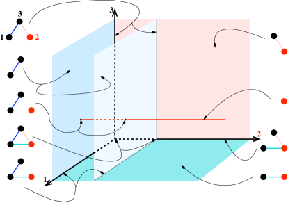
Figure 1. The exponent complexes for $I=\langle\partial_{1}^{2}\partial_{2}^{2}\partial_{3},\partial_{1}\partial_{2}^{2}\partial_{3}^{2}\rangle$.

Example 3.3.

The distraction $\tilde{I}$ of the monomial ideal $I=\langle\partial_{1}^{2}\partial_{2}^{2}\partial_{3},\partial_{1}\partial_{2}^{2}\partial_{3}^{2}\rangle$ has five irreducible components:

$${\mathbb{C}}^{\{1,2\}},\;\;{\mathbb{C}}^{\{2,3\}},\;\;{\mathbb{C}}^{\{1,3\}},\;\;(0,1,0)+{\mathbb{C}}^{\{1,3\}},\;\;(1,0,1)+{\mathbb{C}}^{\{2\}}.$$

On the right and left of Figure 1 we have listed the possible exponent complexes. The first complex on the left is associated to the two vertical lines. The second is associated to the two $\{1,3\}$ planes, the third is associated to the two points $(1,0,1)$ and $(1,1,1)$, the fourth is associated to the two points $(0,0,0)$ and $(0,1,0)$, the fifth is associated to the two lines parallel to the $1$st axis. On the right side, the first complex is associated to the $\{2,3\}$ coordinate plane, the second is associated to all points on the indicated line parallel to the $2$nd axis except for the previously mentioned ones, the third complex is associated to the $2$nd axis, and the last complex is associated to the $\{1,2\}$ coordinate plane.

Example 3.4.

Consider the monomial ideal $I=\langle\partial_{1}^{3}\partial_{2},\partial_{1}^{2}\partial_{2}^{2}\rangle\subseteq{\mathbb{C}}[\partial_{1},\partial_{2}]$, which has primary decomposition $I=\langle\partial_{1}^{2}\rangle\cap\langle\partial_{2}\rangle\cap\langle\partial_{1}^{3},\partial_{2}^{2}\rangle$. The distraction of $I$ is

$$\tilde{I}=\langle\theta_{1}(\theta_{1}-1)(\theta_{1}-2)\theta_{2},\theta_{1}(\theta_{1}-1)\theta_{2}(\theta_{2}-1)\rangle\subseteq{\mathbb{C}}[\theta_{1},\theta_{2}],$$

whose zero set ${\mathbb{V}}(\tilde{I})$ is shown in Figure 2(a), with the irreducible components labeled.

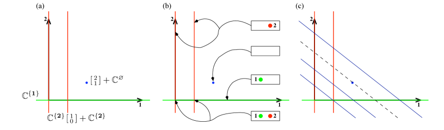
Figure 2. ${\mathbb{V}}(\tilde{I})$ for $I=\langle\partial_{1}^{3}\partial_{2},\partial_{1}^{2}\partial_{2}^{2}\rangle$.

In this example, ${\mathbb{C}}^{\{1\}}$ and $\left[\begin{smallmatrix}1\\ 0\end{smallmatrix}\right]+{\mathbb{C}}^{\{2\}}$ are the two components of ${\mathbb{V}}(\tilde{I})$ that contain the vector $b=\left[\begin{smallmatrix}1\\ 0\end{smallmatrix}\right]$, see Figure 2(b). To this $b$ we associate the simplicial complex $\Delta_{b}(I)=\{\{1\},\{2\},\varnothing\}$, where the numbers 1 and 2 appear because a copy of ${\mathbb{C}}$ appears in the corresponding components listed above. Notice that all of the exponent complexes in Figure 2(b) are 0-dimensional, except for the one associated to $\left[\begin{smallmatrix}2\\ 1\end{smallmatrix}\right]$, which is the empty set and arises because $I$ has an embedded prime.

The connection between the Cohen–Macaulayness of $I$ and the Euler operators can be expressed geometrically. The intersection of the variety ${\mathbb{V}}(\tilde{I})$ with a sufficiently general line consists of 3 points (when counted with multiplicity). The solid slanted lines in Figure 2(c) represent a family of such lines, given by ${\mathbb{V}}(\langle E-\beta\rangle)$ when $A=[\ 1\ 1\ ]$. When $\beta=3$, ${\mathbb{V}}(\langle E-\beta\rangle)$ (the dotted line in Figure 2(c)) passes through the point $\left[\begin{smallmatrix}2\\ 1\end{smallmatrix}\right]$. This results in an intersection multiplicity of 4 with ${\mathbb{V}}(\tilde{I})$, confirming the non-Cohen–Macaulayness of $I$.

For a general monomial ideal $I$, such a jump in intersection multiplicity between ${\mathbb{V}}(\tilde{I})$ and the $(n-d)$-dimensional linear space ${\mathbb{V}}(\langle E-\beta\rangle)$ can occur in two different ways. As we have just witnessed, if $I$ is not unmixed, a non-generic intersection involving a lower dimensional component of ${\mathbb{V}}(\tilde{I})$ will have more points than expected, as we have just seen. Also, even if $I$ is unmixed, some non-generic points of ${\mathbb{V}}(\tilde{I})$ could contribute a higher multiplicity to the intersection (see Example 3.16). We show in Theorem 3.11 that this is the case precisely at the points $b$ where $\Delta_{b}(I)$ fails to be a Cohen–Macaulay simplicial complex.

Definition 3.5.

Given a simplicial complex $\Delta$ on $\{1,\dots,n\}$, the Stanley-Reisner ring or face ring of $\Delta$ is ${\mathbb{C}}[\theta]/I_{\Delta}$, where

$$I_{\Delta}:=\bigcap\ \langle\theta_{j}:j\notin\sigma\rangle$$

and the intersection runs over the facets $\sigma$ of $\Delta$. Note that $I_{\Delta}$ is a squarefree monomial ideal, and any squarefree monomial ideal can be obtained in this manner. The Krull dimension of ${\mathbb{C}}[\theta]/I_{\Delta}$ is the maximal cardinality of a facet of $\Delta$, hence $\dim({\mathbb{C}}[\theta]/I_{\Delta})=\dim(\Delta)+1$.

Definition 3.6.

For an exponent $b$ of $I$, let $J_{b}:=I_{\Delta_{b}(I)}\subseteq{\mathbb{C}}[\theta]$ denote the Stanley–Reisner ideal of the exponent complex $\Delta_{b}(I)$, and $J_{b}(\theta-b)$ denote the ideal obtained from $J_{b}$ by replacing $\theta_{i}$ with $\theta_{i}-b_{i}$. Note that

$$J_{b}(\theta-b)=\bigcap\langle\theta_{i}-b_{i}\mid i\notin\sigma\rangle,$$

where the intersection runs over the facets of $\Delta_{b}(I)$, equivalently, over the $\sigma\subseteq\{1,\dots,n\}$ such that $b+{\mathbb{C}}^{\sigma}$ is an irreducible component of ${\mathbb{V}}(\tilde{I})$.

We now recall Reisner’s criterion for the Cohen–Macaulayness of Stanley–Reisner rings; proofs of this fact can be found in [BH93, Corollary 5.3.9], [Sta96, Section II.4], and [MS05, Section 13.5.2].

Definition 3.7.

Let $\Delta$ be a simplicial complex and $\sigma\in\Delta$. The link of $\sigma$ is the simplicial complex

$${\rm lk\ }\sigma=\{\tau\in\Delta\mid\sigma\cup\tau\in\Delta,\sigma\cap\tau=\varnothing\}.$$

Theorem 3.8.

Given a simplicial complex $\Delta$, its Stanley–Reisner ring ${\mathbb{C}}[\theta]/I_{\Delta}$ is Cohen–Macaulay if and only if ${\widetilde{H}}_{i}({\rm lk\ }\sigma;{\mathbb{C}})=0$ for all $\sigma\in\Delta$ and for all $i<\dim({\rm lk\ }\sigma)$.

Definition 3.9.

A simplicial complex $\Delta$ is Cohen–Macaulay if and only if its Stanley–Reisner ring is Cohen–Macaulay; equivalently, when $\Delta$ satisfies the condition in Theorem 3.8.

We will use the following fact in the proof of Theorem 3.11.

Proposition 3.10.

[BH93, Corollary 4.6.11] Let $J$ be a homogeneous ideal in ${\mathbb{C}}[\theta]$. If $E$ is a linear system of parameters for ${\mathbb{C}}[\theta]/J$, then

$$\deg(J)\leq\deg(J+\langle E\rangle)=\dim_{{\mathbb{C}}}({\mathbb{C}}[\theta]/(J+\langle E\rangle)),$$

and equality holds if and only if $J$ is Cohen–Macaulay.

The following result is an adaptation of [SST00, Theorem 4.6.1].

Theorem 3.11.

Given a monomial ideal $I\subseteq{\mathbb{C}}[\partial]$ and $\beta\in{\mathbb{C}}^{d}$,

$$\dim_{\mathbb{C}}\left(\frac{{\mathbb{C}}[\theta]}{\tilde{I}+\langle E-\beta\rangle}\right)=\deg(I)$$

if and only if $\Delta_{b}(I)$ is a Cohen–Macaulay complex of dimension $d-1$ for all $b\in{\mathbb{V}}(\tilde{I}+\langle E-\beta\rangle)$.

Proof.

Since $\tilde{I}+\langle E-\beta\rangle=\bigcap_{b\in{\mathbb{V}}(\tilde{I}+\langle E-\beta\rangle)}J_{b}(\theta-b)+\langle E-\beta\rangle$,

$$\dim_{{\mathbb{C}}}({\mathbb{C}}[\theta]/(\tilde{I}+\langle E-\beta\rangle))=\sum_{b\in{\mathbb{V}}(\tilde{I}+\langle E-\beta\rangle)}\dim_{{\mathbb{C}}}({\mathbb{C}}[\theta]/(J_{b}+\langle E\rangle)).$$

Proposition 3.10 implies that for any $b\in{\mathbb{V}}(\tilde{I}+\langle E-\beta\rangle)$ such that $\dim({\mathbb{C}}[\theta]/(J_{b}))=d$,

$$\dim_{{\mathbb{C}}}({\mathbb{C}}[\theta]/(J_{b}+\langle E\rangle))\geq\deg(J_{b}),$$

with equality if and only if $J_{b}$ is Cohen–Macaulay. By summing over the exponents $b$ of $I$ corresponding to $\beta$, we obtain the inequality

$$\dim_{{\mathbb{C}}}({\mathbb{C}}[\theta]/(\tilde{I}+\langle E-\beta\rangle))=\sum_{b\in{\mathbb{V}}(\tilde{I}+\langle E-\beta\rangle)}\dim_{{\mathbb{C}}}({\mathbb{C}}[\theta]/(J_{b}+\langle E\rangle))\geq\sum_{\dim({\mathbb{C}}[\theta]/J_{b})=d}\deg(J_{b}).$$

Notice that the right hand sum is

$$\sum_{\dim({\mathbb{C}}[\theta]/J_{b})=d}\deg(J_{b})=\deg(I)$$

because the degree of a monomial ideal is equal to the number of top dimensional irreducible components of its distraction. Therefore

$$\dim_{{\mathbb{C}}}\left(\frac{{\mathbb{C}}[\theta]}{\tilde{I}+\langle E-\beta\rangle}\right)\geq\deg(I),$$

with equality if and only if for all $b\in{\mathbb{V}}(\tilde{I}+\langle E-\beta\rangle)$ with $\dim({\mathbb{C}}[\theta]/J_{b})=d$, we have that $\dim_{{\mathbb{C}}}({\mathbb{C}}[\theta]/(J_{b}+\langle E\rangle))=\deg(J_{b})$. If $\dim({\mathbb{C}}[\theta]/J_{b})=d$, then $E$ is a linear system of parameters for $J_{b}$ and

$$\dim_{{\mathbb{C}}}({\mathbb{C}}[\theta]/(J_{b}+\langle E\rangle))\geq\deg(J_{b}),$$

with equality if and only if ${\mathbb{C}}[\theta]/J_{b}$ is Cohen–Macaulay, by Proposition 3.10. Hence we have $\dim_{{\mathbb{C}}}({\mathbb{C}}[\theta]/(\tilde{I}+\langle E-\beta\rangle))=\deg(I)$ exactly when ${\mathbb{C}}[\theta]/J_{b}$ is Cohen–Macaulay of Krull dimension $d$ for all $b\in{\mathbb{V}}(\tilde{I}+\langle E-\beta\rangle$. Finally, recall that by definition $\Delta_{b}(I)$ is Cohen–Macaulay of dimension $d-1$ when $J_{b}=I_{\Delta_{b}(I)}$ is Cohen–Macaulay of dimension $d$. ∎

The main result of this section now follows directly from Corollary 2.15 and Theorem 3.11. Recall from Remark 3.2 that there are finitely many exponent complexes $\Delta_{b}(I)$ that can be obtained after consideration of finitely many exponents $b\in{\mathbb{Z}}^{n}$.

Theorem 3.12.

A $d$-dimensional monomial ideal $I$ is Cohen–Macaulay if and only if its (finitely many) exponent complexes are Cohen–Macaulay of dimension $d-1$.

Remark 3.13.

If $I=I_{\Delta}$ is squarefree and $\Delta_{0}(I)=\Delta$ is Cohen–Macaulay, then Theorem 3.8 and Theorem 3.12 together imply that all exponent complexes of $I$ are Cohen–Macaulay of dimension $d-1$.

Example 3.14 (Example 3.3, continued).

The third simplicial complex on the left in Figure 1 is not Cohen–Macaulay by Theorem 3.8 because the link of the empty set is one-dimensional and ${\widetilde{H}}_{0}({\rm lk\ }\varnothing;{\mathbb{C}})={\mathbb{C}}\neq 0$. It now follows from Theorem  3.12 that $I$ is not Cohen–Macaulay.

Example 3.15 (Example 3.4, continued).

For $b=\left[\begin{smallmatrix}2\\ 1\end{smallmatrix}\right]$, $\Delta_{b}(I)$ is empty, while $d=2$. Thus by Theorem 3.12, $I$ is not Cohen–Macaulay.

It is well-known that the Cohen–Macaulay property of a monomial ideal is inherited by its radical (see [Tay02, Proposition 3.1] or [HTT, Theorem 2.6]); however, the converse is not true. Theorem 3.12 provides the conditions necessary to obtain a converse, as $\Delta_{0}(I)$ is the Stanley–Reisner complex for the radical of $I$.

Example 3.16.

Consider the monomial ideal

$$I=\langle\partial_{1}\partial_{4},\partial_{2}\partial_{4},\partial_{2}\partial_{3},\partial_{1}\partial_{3}\partial_{5},\partial_{5}^{2}\rangle\subseteq{\mathbb{C}}[\partial_{1},\dots,\partial_{5}].$$

The irreducible components of ${\mathbb{V}}(\tilde{I})$ are

$${\mathbb{C}}^{\{1,2\}},\;\;{\mathbb{C}}^{\{1,3\}},\;\;{\mathbb{C}}^{\{3,4\}},\;\;(0,0,0,0,1)+{\mathbb{C}}^{\{1,2\}},\;\;(0,0,0,0,1)+{\mathbb{C}}^{\{3,4\}}.$$

For $b=(0,0,0,0,1)$, the simplicial complex $\Delta_{b}(I)$ consists of two line segments, $\{1,2\}$ and $\{3,4\}$. The link of the empty set is all of $\Delta_{b}(I)$, a one-dimensional simplicial complex with nonvanishing zeroth reduced homology; this implies that $\Delta_{b}(I)$ is not Cohen–Macaulay by Theorem 3.8. Thus, while $I$ is unmixed and $\sqrt{I}$ is Cohen–Macaulay, Theorem 3.12 implies that $I$ is not Cohen-Macaulay.

By introducing new variables, one can pass from the monomial ideal $I\subseteq{\mathbb{C}}[\partial]$ to its polarization, a squarefree monomial ideal $I_{\Delta}$ in a larger polynomial ring $S$ such that $S/(I_{\Delta}+\langle y\rangle)\cong{\mathbb{C}}[\partial]/I$ for some regular sequence $y$ in $S/I_{\Delta}$. In particular, $I$ is Cohen–Macaulay if and only if the single simplicial complex $\Delta$ is Cohen–Macaulay. However, the number of variables in $S$ can make the application of Theorem 3.8 to $\Delta$ much more computationally expensive than checking the Cohen–Macaulayness of the finitely many $\Delta_{b}(I)$ of Theorem 3.12. This is the case in the following family of monomial ideals from [Jar02].

Example 3.17.

Given $k\in{\mathbb{N}}$, let $m_{i}=\prod_{j\neq i}\partial_{j}^{k}$, and consider the ideal

$$I_{k}=\langle m_{1},\dots,m_{n}\rangle\subseteq{\mathbb{C}}[\partial_{1},\dots,\partial_{n}].$$

Jarrah shows that ${\mathbb{C}}[\partial]/I_{k}$ is Cohen–Macaulay by explicitly constructing the minimal free resolution. Let us verify this fact combinatorially.

By Theorem 3.12, we only need to check that ${\mathbb{C}}[\partial]/I_{1}$ is Cohen–Macaulay, as the exponent complexes of $I_{k}$ and $I_{1}$ are the same. But $I_{1}$ is squarefree, so it is enough to show that $\Delta_{0}(I_{1})$ is a Cohen–Macaulay simplicial complex (of dimension $n-3$). Now

$$\Delta_{0}(I_{1})=\{\sigma\subseteq\{1,\dots,n\}\ \big{|}\ |\sigma|\leq n-2\}.$$

The link of $\sigma\in\Delta_{0}(I_{1})$ consists of subsets of $\{1,\dots,n\}\smallsetminus\sigma$ of cardinality at most $n-2-|\sigma|$. This simplicial complex is homotopy equivalent to a wedge of $(n-3-|\sigma|)$-spheres, whose only nonvanishing reduced homology occurs in the top degree. Thus $\Delta_{0}(I_{1})$ is Cohen–Macaulay.

On the other hand, the polarization of $I_{k}$ is much less transparent. For instance, if $k=4$ and $n=4$, the polarization of $I_{4}=\langle\partial_{1}^{4}\partial_{2}^{4}\partial_{3}^{4},\partial_{1}^{4}\partial_{2}^{4}\partial_{4}^{4},\partial_{1}^{4}\partial_{3}^{4}\partial_{4}^{4},\partial_{2}^{4}\partial_{3}^{4}\partial_{4}^{4}\rangle$ is

$$I_{\Delta}=\ \langle s_{1}s_{2}s_{3}s_{4}t_{1}t_{2}t_{3}t_{4}u_{1}u_{2}u_{3}u_{4},s_{1}s_{2}s_{3}s_{4}t_{1}t_{2}t_{3}t_{4}v_{1}v_{2}v_{3}v_{4},$$

$$\ \ s_{1}s_{2}s_{3}s_{4}u_{1}u_{2}u_{3}u_{4}v_{1}v_{2}v_{3}v_{4},t_{1}t_{2}t_{3}t_{4}u_{1}u_{2}u_{3}u_{4}v_{1}v_{2}v_{3}v_{4}\rangle$$

$$\subseteq{\mathbb{C}}[s_{1},s_{2},s_{3},s_{4},t_{1},t_{2},t_{3},t_{4},u_{1},u_{2},u_{3},u_{4},v_{1},v_{2},v_{3},v_{4}],$$

where, for example, $\partial_{1}^{4}$ has been replaced by $s_{1}s_{2}s_{3}s_{4}$. The $f$-vector $(f_{-1},f_{0},f_{1},\dots)$ of $\Delta$ is

$$f(\Delta)=(1,16,120,560,1820,4368,8008,11440,12870,11440,8008,4368,1816,544,96),$$

where $f_{i}$ is the number of faces of $\Delta$ of dimension $i$. Applying Reisner’s criterion to verify the Cohen–Macaulayness of $\Delta$ is computationally expensive, especially in comparison with verification via Theorem 3.12, which involves only $1$-dimensional simplicial complexes on four vertices.

Remark 3.18.

There are several known families of simplicial complexes that capture homological properties of $I$, including those in [BH93, Theorems 5.3.8 and 5.5.1], [Mus00], [MS05, Theorems 1.34 and 5.11], and [Tak05]. See [Mil08] for details on how these relate to each other and to the exponent complexes $\Delta_{b}(I)$.

4. A combinatorial formula for rank

For the remainder of this article, we work over any field ${\Bbbk}$ of characteristic zero. The ${\Bbbk}$-vector space dimension of ${\Bbbk}[\theta]/(\tilde{I}+\langle E-\beta\rangle)$ measures the deviation (with respect to $\beta\in{\Bbbk}^{d}$) of the ideal $I$ from being Cohen–Macaulay. The goal of this section is to explicitly compute this dimension, which equals ${\rm rank\ }(I+\langle E-\beta\rangle)$ when ${\Bbbk}={\mathbb{C}}$, by Lemma 2.12.

We first observe that the dimension we wish to compute is equal to the sum over the exponents $b\in{\mathbb{V}}(\tilde{I}+\langle E-\beta\rangle)$ of the ${\Bbbk}$-vector space dimensions of ${\Bbbk}[\theta]/(I_{\Delta_{b}(I)}+\langle E\rangle)$. This reduces the computation to the case that $\tilde{I}$ is squarefree and $\beta=0$.

Proposition 4.1.

Let $I$ be a monomial ideal in ${\Bbbk}[\partial]$, not necessarily squarefree. Then

$$\dim_{\Bbbk}\left(\frac{{\Bbbk}[\theta]}{\tilde{I}+\langle E-\beta\rangle}\right)=\sum_{b\in{\mathbb{V}}(\tilde{I}+\langle E-\beta\rangle)}\dim_{\Bbbk}\left(\frac{{\Bbbk}[\theta]}{I_{\Delta_{b}(I)}+\langle E\rangle}\right).$$

Proof.

Recall that for $b\in{\mathbb{V}}(\tilde{I}+\langle E-\beta\rangle)$, $I_{\Delta_{b}(I)}=J_{b}\subseteq{\Bbbk}[\theta]$ denotes the Stanley–Reisner ideal of $\Delta_{b}(I)$. Since $\tilde{I}+\langle E-\beta\rangle=\bigcap_{b\in{\mathbb{V}}(\tilde{I}+\langle E-\beta\rangle)}J_{b}(\theta-b)+\langle E-\beta\rangle$, the ${\Bbbk}$-vector space dimension of ${\Bbbk}[\theta]/(\tilde{I}+\langle E-\beta\rangle)$ is equal to the sum over all exponents of $I$ with respect to $\beta$ of the dimensions of ${\Bbbk}[\theta]/(J_{b}(\theta-b)+\langle E-\beta\rangle)$. Each of these clearly coincides with the dimension of ${\Bbbk}[\theta]/(J_{b}+\langle E\rangle)$. ∎

4.1. The squarefree case

Henceforth, $I=I_{\Delta}$ is the squarefree monomial ideal in ${\Bbbk}[\theta]$ corresponding to a simplicial complex $\Delta$ on $\{1,\dots,n\}$.

Notation 4.2.

Let $F^{0}$ denote the set of facets of $\Delta$, and for $p>0$, set

(4.1) $$F^{p}=\{s\subseteq F^{0}\ \big{|}\ |s|=p+1\}.$$

Each element $s\in F^{p}$ determines a face

$$\sigma(s)=\bigcap_{\tau\in s}\tau\ \in\Delta.$$

Note that $\sigma(F^{0})=\bigcap_{s\in F^{0}}\sigma(s)$ is the face of $\Delta$ corresponding to the unique element of $F^{|F^{0}|-1}$. For $S\subseteq F^{p}$, we denote by

(4.2) $$\kappa(S)=\max\left(0,\ d-\bigg{|}\bigcup_{s\in S}\sigma(s)\bigg{|}\right),$$

(see also Notation 4.8). Finally, we give notation to describe the $(p+1)$-intersections of facets of $\Delta$ that have dimension less than $d-p$:

(4.3) $$G^{p}=\{s\in F^{p}\mid\kappa(s)\geq p+1\}.$$

Definition 4.3.

The collections $F^{\bullet}$ naturally correspond to the nonempty faces of a $(|F^{0}|-1)$-simplex $\Omega$; we may view a subset $S\subseteq G^{p}$ as a collection of $p$-faces of $\Omega$. Given $t\in G^{p}\setminus S$, we abuse notation and write $S$ and $S\cup\{t\}$ for the subcomplexes of $\Omega$ whose maximal faces are given by these sets. Suppose that there is a minimal generator of $H^{p}(S\cup\{t\},S;{\Bbbk})$ of the form $\sum_{s\in S}v_{s}\cdot s+v_{t}\cdot t$, where all coefficients are nonzero. In this case, we say that $S\cup\{t\}$ is a circuit for $t$.

Notation 4.4.

Let $G^{p}=\{s_{1},s_{2},\dots,s_{|G^{p}|}\}$ be a fixed order on $G^{p}$. For $1\leq j<|G^{p}|$, set

$$G^{p}(j) =\{s_{1},\dots,s_{j}\},$$

$$L^{p}(j) =\{\tau\subseteq\{1,\dots,j+1\}\mid\{s_{i}\}_{i\in\tau}\text{ is a circuit for $s_{j+1}$},\ j+1\in\tau\},$$

$$\text{ and }\quad L^{p}(j,k) =\{\Lambda\subseteq L^{p}(j)\mid|\Lambda|=k\}\text{ for $1\leq k\leq|L^{p}(j)|$. }$$

For $\Lambda\in L^{p}(j,k)$, let $s_{\Lambda}=\bigcup_{\tau\in\Lambda}\bigcup_{i\in\tau}s_{i}$, and define

$$\psi^{p}(j)= \sum_{k=1}^{|L^{p}(j)|}\sum_{\Lambda\in L^{p}(j,k)}(-1)^{|\Lambda|+1}\binom{\kappa(s_{\Lambda})}{p+1}$$

Adding over all $j$, we obtain

$$\psi^{p}=\sum_{j=1}^{|G^{p}|-1}\psi^{p}(j).$$

This notation is designed for the proof of Lemma 4.19, where its motivation will become clear.

The derivation of the following formula will occupy the remainder of this section.

Theorem 4.5.

If $I=I_{\Delta}$ is a squarefree monomial ideal in ${\Bbbk}[\theta]$, then

$$\dim_{\Bbbk}\left(\frac{{\Bbbk}[\theta]}{I+\langle E\rangle}\right)=\deg(I)+\binom{\kappa(\sigma(F^{0}))-1}{|F^{0}|-1}-\sum_{p=0}^{|F^{0}|-2}\sum_{s\in G^{p}}\binom{\kappa(s)-1}{p+1}+\sum_{p=0}^{|F^{0}|-2}\psi^{p}.$$

Remark 4.6.

The set of top-dimensional faces of $\Delta$ is $F^{0}\setminus G^{0}=\{s\in F^{0}\mid|\sigma(s)|=d\}$ because $\dim(\Delta)=d-1$, and the degree of $I$ is

$$\deg(I)=\sum_{s\in F^{0}\setminus G^{0}}\binom{\kappa(s)}{0}=|F^{0}\setminus G^{0}|.$$

Example 4.7 (Example 3.16, continued).

With $b=(0,0,0,0,1)$, consider the squarefree ideal $I_{\Delta_{b}(I)}\subseteq{\Bbbk}[\theta_{1},\dots,\theta_{5}]$. Recall that the simplicial complex $\Delta_{b}(I)$ consists of two line segments, $\{1,2\}$ and $\{3,4\}$, so $F^{0}=\{s=\{1,2\},s^{\prime}=\{3,4\}\}$, $F^{1}=\{\{s,s^{\prime}\}\}$, and $F^{p}=0$ for $p\neq 0,1$. Also, $G^{0}=\varnothing$. By Theorem 4.5,

$$\dim_{\Bbbk}\left(\frac{{\Bbbk}[\theta]}{I_{\Delta_{b}(I)}+\langle E\rangle}\right)= \ 2+\binom{1}{1}-0+0=3.$$

To prove Theorem 4.5, we begin by constructing an acyclic cochain complex, called the primary resolution of $I=I_{\Delta}$ because its only homology module is isomorphic to ${\Bbbk}[\theta]/I$. We will then consider the resulting Koszul spectral sequence with respect to $E$.

Notation 4.8.

The submatrix of $A$ with columns corresponding to a face $\sigma\in\Delta$ is denoted $A_{\sigma}=(a_{i})_{i\in\sigma}$, and ${\Bbbk}[\theta_{\sigma}]={\Bbbk}[\theta_{i}\mid i\in\sigma]$ is a polynomial ring in the corresponding variables. We view ${\Bbbk}[\theta_{\sigma}]$ as a ${\Bbbk}[\theta]$-module via the natural surjection ${\Bbbk}[\theta]\twoheadrightarrow{\Bbbk}[\theta]/\langle\theta_{i}\mid i\notin\sigma\rangle={\Bbbk}[\theta_{\sigma}]$. For $s\in F^{p}$, $\dim{\Bbbk}[\theta_{\sigma(s)}]=|\sigma(s)|=\dim_{\Bbbk}({\Bbbk}A_{\sigma(s)})$ by our assumptions on $A$ in Convention 2.7. Thus $\kappa(s)$ from Notation 4.2 is equal to ${\rm codim}_{{\Bbbk}^{d}}({\Bbbk}A_{\sigma(s)})$.

By choice of a suitable incidence function on the lattice $F^{\bullet}$, there is an exact sequence of ${\Bbbk}[\theta]$-modules:

(4.4) $$0\rightarrow{\Bbbk}[\theta]/I\rightarrow R^{\bullet},$$

where

(4.5) $$R^{p}=\bigoplus_{s\in F^{p}}{\Bbbk}[\theta_{\sigma(s)}].$$

We call $R^{\bullet}$ the primary resolution of $I$. We may view $R^{\bullet}$ as a cellular resolution supported on an $(|F^{0}|-1)$-simplex (see [Ber08, Definition 6.7]).

Example 4.9 (Example 4.7, continued).

In this case, the primary resolution of $I$ will be

$${\Bbbk}[\theta_{1},\theta_{2}]\oplus{\Bbbk}[\theta_{3},\theta_{4}]\stackrel{{\scriptstyle\delta}}{{\longrightarrow}}{\Bbbk}\longrightarrow 0$$

with differential $\delta(f,g)={\overline{f}}-{\overline{g}}$, where ${\overline{\phantom{}\cdot\phantom{}}}$ denotes image modulo $\langle\theta\rangle$.

Remark 4.10.

The primary resolution $R^{\bullet}$ of (4.4) is an example of an irreducible resolution of ${\Bbbk}[\theta]/I$ in [Mil02, Definition 2.1]. [Mil02, Theorem 4.2] shows that $I$ is Cohen–Macaulay precisely when $R^{\bullet}$ contains an irreducible resolution $S^{\bullet}$ of ${\Bbbk}[\theta]/I$ such that $S^{p}$ is of pure Krull dimension $\dim(I)-p$ for all $p\geq 0$. If this is the case, then by Corollary 2.15, the ${\Bbbk}$-vector space dimension of ${\Bbbk}[\theta]/(I+\langle E\rangle)$ is equal to the degree of $I$. However, our current computation of $\dim_{\Bbbk}({\Bbbk}[\theta]/(I+\langle E\rangle))$ is independent of this remark.

Remark 4.11.

While the primary resolution $R^{\bullet}$ of $I$ may appear to be similar to the complex in [BH93, Theorem 5.7.3], they are generally quite different. For each $\sigma$, this other complex places ${\Bbbk}[\theta_{\sigma}]$ in the $|\sigma|$-th homological degree. However, $R^{\bullet}$ permits summands of rings of varying Krull dimension within a single cohomological degree and ${\Bbbk}[\theta_{\sigma}]$ never appears in the primary resolution if $\sigma$ is not contained in the intersection of a collection of facets of $\Delta$. In fact, the primary resolution will coincide with (a shifted copy of) the complex in [BH93, Theorem 5.7.3] only when $\Delta$ is the boundary of a simplex.

Consider the double complex $E_{0}^{\bullet,\bullet}$ given by $E_{0}^{p,-q}=K_{q}(R^{p};E)$, where $K_{\bullet}(-;E)$ forms a Koszul complex with respect to the sequence $E$. Taking homology first with respect to the horizontal differential, we see that

$${}_{h}E_{\infty}^{p,-q}={}_{h}E_{1}^{p,-q}=\begin{cases}K_{q}({\Bbbk}[\theta]/I;E)&\text{if $p=0\text{ and }0\leq q\leq d,$}\\ 0&\text{otherwise.}\end{cases}$$

Let ${}_{v}E_{\bullet}^{\bullet,\bullet}$ denote the spectral sequence obtained from $E_{0}^{\bullet,\bullet}$ by first taking homology with respect to the vertical differential. Since $H_{0}({\Bbbk}[\theta]/I;E)={\Bbbk}[\theta]/(I+\langle E\rangle)$ and ${}_{v}E_{\bullet}^{\bullet,\bullet}$ converges to the same abutment as ${}_{h}E_{\bullet}^{\bullet,\bullet}$,

(4.6) $$\dim_{\Bbbk}\left(\frac{{\Bbbk}[\theta]}{I+\langle E\rangle}\right)=\sum_{p-q=0}\dim_{\Bbbk}({}_{v}E_{\infty}^{p,-q}).$$

Notice that

$${}_{v}E_{1}^{p,-q}=\begin{cases}H_{q}(R^{p};E)&\text{if $0\leq q\leq d,$}\\ 0&\text{otherwise,}\end{cases}$$

and for $0\leq q\leq d$,

$$H_{q}(R^{p};E)=\bigoplus_{s\in F^{p}}H_{q}({\Bbbk}[\theta_{\sigma(s)}];E).$$

Instead of ${}_{v}E_{\bullet}^{\bullet,\bullet}$, we will study a sequence ${{}^{\prime}E}_{\bullet}^{\bullet,\bullet}$ with the same abutment and differentials which behave well with respect to vanishing of Koszul homology. To introduce this sequence, we first need some notation.

Notation 4.12.

For $\sigma\in\Delta$, let $L(\sigma)$ be the lexicographically first subset of $\{1,2,\dots,d\}$ of cardinality equal to $\dim_{\Bbbk}({\Bbbk}A_{\sigma})$ such that $\{E_{i}\}_{i\in L(\sigma)}$ is a system of parameters for ${\Bbbk}[\theta_{\sigma}]$ (as a ${\Bbbk}[\theta]$-module). For a ${\mathbb{Z}}$-graded ${\Bbbk}[\theta_{\sigma}]$-module $M$, let $K^{\sigma}_{\bullet}(M;E)$ denote the Koszul complex on $M$ given by the operators $\{E_{i}\}_{i\in L(\sigma)}$ and $H^{\sigma}_{q}(M;E)=H_{i}(K^{\sigma}_{\bullet}(M;E))$.

Notation 4.13.

For $\sigma\in\Delta$, let

$$\ker_{\mathbb{Z}}A_{\sigma}=\{v\in{\mathbb{Z}}^{d}\mid\sum_{i=1}^{d}v_{i}a_{ij}=0\ \forall j\in\sigma\},$$

using the standard basis of ${\mathbb{Z}}A={\mathbb{Z}}^{d}$, and let $\bigwedge^{\bullet}(\ker_{\mathbb{Z}}A_{\sigma})$ denote a complex with trivial differentials. These complexes will be useful in our computation of $\dim_{\Bbbk}({\Bbbk}[\theta]/(I+\langle E\rangle))$.

Lemma 4.14.

Let $\sigma\in\Delta$ and $M$ be an $A$-graded ${\Bbbk}[\theta_{\sigma}]$-module. There is a quasi-isomorphism of complexes

(4.7) $$K_{\bullet}(M;E)\simeq_{\text{qis}}K^{\sigma}_{\bullet}(M;E)\otimes_{\mathbb{Z}}\bigwedge^{\bullet}\left(\ker_{\mathbb{Z}}A_{\sigma}\right).$$

In particular, there is a decomposition $H_{\bullet}({\Bbbk}[\theta_{\sigma}];E)\cong H^{\sigma}_{0}({\Bbbk}[\theta_{\sigma}];E)\otimes_{\mathbb{Z}}\bigwedge^{\bullet}\left(\ker_{\mathbb{Z}}A_{\sigma}\right).$

Proof.

The quasi-isomorphism (4.7) is a commutative version of Proposition 3.3 in [Ber08]. Since $\dim_{\Bbbk}({\Bbbk}A_{\sigma})=|\sigma|=\dim{\Bbbk}[\theta_{\sigma}]$, the choice of $L(\sigma)$ implies that $\{E_{i}\}_{i\in L(\sigma)}$ is a maximal ${\Bbbk}[\theta_{\sigma}]$-regular sequence. Thus the second statement follows from [BH93, Corollary 1.6.14]. ∎

Lemma 4.15.

Let $\sigma\subseteq\tau$ be faces of $\Delta$, and let $\pi:{\Bbbk}[\theta_{\tau}]\twoheadrightarrow{\Bbbk}[\theta_{\sigma}]$ be the natural surjection. There is a commutative diagram

(4.12)

with vertical maps given by (4.7). Further, the image of $H_{\bullet}(\pi;E)$ is isomorphic to

$$H^{\sigma}_{0}({\Bbbk}[\theta_{\sigma}];E)\otimes_{\mathbb{Z}}\bigwedge^{\bullet}\left(\ker_{\mathbb{Z}}A_{\tau}\right)$$

as a submodule of $H^{\sigma}_{0}(N;E)\otimes_{\mathbb{Z}}\bigwedge^{\bullet}\left(\ker_{\mathbb{Z}}A_{\sigma}\right)$.

Proof.

This is a modified version of Lemma 3.7 and Proposition 3.8 in [Ber08]. ∎

Notation 4.16.

Let $({{}^{\prime}E}_{\bullet}^{\bullet,\bullet},\delta_{\bullet}^{\bullet,\bullet})$ be the spectral sequence determined by letting $\delta_{0}^{\bullet,\bullet}$ be the vertical differential of the double complex ${{}^{\prime}E}_{0}^{\bullet,\bullet}$ with

$${{}^{\prime}E}_{0}^{p,-q}=\bigoplus_{s\in F^{p}}\bigoplus_{i+j=q}K^{\sigma}_{i}({\Bbbk}[\theta_{\sigma(s)}];E)\otimes_{\mathbb{Z}}\bigwedge^{j}\left(\ker_{\mathbb{Z}}A_{\sigma(s)}\right).$$

Note that by Lemma 4.14,

(4.13) $${{}^{\prime}E}_{1}^{p,-q}=\bigoplus_{s\in F^{p}}H^{\sigma}_{0}({\Bbbk}[\theta_{\sigma(s)}];E)\otimes_{\mathbb{Z}}\bigwedge^{q}\left(\ker_{\mathbb{Z}}A_{\sigma(s)}\right).$$

By Lemmas 4.14 and 4.15, the horizontal differentials of $E_{0}^{\bullet,\bullet}$ are compatible with the quasi-isomorphism

$$E_{0}^{p,\bullet}\simeq_{qis}\bigoplus_{s\in F^{p}}K^{\sigma}_{\bullet}({\Bbbk}[\theta_{\sigma(s)}];E)\otimes_{\mathbb{Z}}\bigwedge^{\bullet}\left(\ker_{\mathbb{Z}}A_{\sigma(s)}\right).$$

Thus we may replace ${}_{v}E_{\infty}^{p,-q}$ in (4.6) with ${{}^{\prime}E}_{\infty}^{p,-q}$, obtaining

(4.14) $$\dim_{\Bbbk}\left(\frac{{\Bbbk}[\theta]}{I+\langle E\rangle}\right)=\sum_{p-q=0}\dim_{\Bbbk}({{}^{\prime}E}_{\infty}^{p,-q}).$$

This replacement is beneficial because ${{}^{\prime}E}_{\bullet}^{\bullet,\bullet}$ degenerates quickly.

Lemma 4.17.

The spectral sequence ${{}^{\prime}E}_{\bullet}^{\bullet,\bullet}$ of (4.13) degenerates at the second page: ${}^{\prime}E_{2}^{\bullet,\bullet}={{}^{\prime}E}_{\infty}^{\bullet,\bullet}.$

Proof.

The proof follows the same argument as [Ber08, Lemma 5.26]. ∎

Lemma 4.17 and (4.14) imply that

(4.15) $$\dim_{\Bbbk}\left(\frac{{\Bbbk}[\theta]}{I+\langle E\rangle}\right)=\sum_{p-q\geq 0}(-1)^{p-q}\dim_{\Bbbk}({{}^{\prime}E}_{1}^{p,-q})-\sum_{p-q=-1}\dim_{\Bbbk}({\rm image\ }\delta_{1}^{p,-q}),$$

and recall from Notation 4.16 that $\delta_{\bullet}^{\bullet,\bullet}$ denotes the differential of ${{}^{\prime}E}_{\bullet}^{\bullet,\bullet}$. We compute the dimensions on the right hand side of (4.15) in the following lemmas.

Lemma 4.18.

For $0\leq q\leq d$ and $p\geq 0$,

$$\dim_{\Bbbk}({{}^{\prime}E}_{1}^{p,-q})=\sum_{s\in F^{p}}\binom{\kappa(s)}{q}.$$

Proof.

By Lemma 4.14,

$${{}^{\prime}E}_{1}^{p,-q}=\bigoplus_{s\in F^{p}}H^{\sigma}_{0}({\Bbbk}[\theta_{\sigma(s)}];E)\otimes_{\mathbb{Z}}\bigwedge^{q}\left(\ker_{\mathbb{Z}}A_{\sigma(s)}\right).$$

Since $\{E_{i}\}_{i\in L_{\sigma(s)}}$ is a system of parameters for ${\Bbbk}[\theta_{\sigma(s)}]$ for all $s\in F^{p}$, the ${\Bbbk}$-vector space dimension of the module $H^{\sigma}_{0}({\Bbbk}[\theta_{\sigma(s)}];E)$ is $1$. Hence

$$\dim_{\Bbbk}({{}^{\prime}E}_{1}^{p,-q})=\sum_{s\in F^{p}}\binom{{\rm codim}_{{\Bbbk}^{d}}({\Bbbk}A_{\sigma(s)})}{q},$$

and by the choice of $A$ in Convention 2.7, $\kappa(s)={\rm codim}_{{\Bbbk}^{d}}({\Bbbk}A_{\sigma(s)})$. ∎

Lemma 4.19.

For $p\leq|F^{0}|-2$,

(4.16) $$\dim_{\Bbbk}({\rm image\ }\delta_{1}^{p,-p-1})=-\psi^{p}+\sum_{s\in G^{p}}\binom{\kappa(s)}{p+1}.$$

Proof.

We first note that if $p>|F^{0}|-2$, then $R^{p+1}=0$ and ${\rm image\ }\delta_{1}^{p,-p-1}=0$.

Now with $0\leq p\leq|F^{0}|-2$, fix an order for the elements of $G^{p}$, say

$$G^{p}=\{s_{1},s_{2},\dots,s_{|G^{p}|}\},$$

as in Notation 4.4. For a subset $S\subseteq G^{p}$, let $\delta_{1,S}^{p,-q}$ denote the restriction of $\delta_{1,S}^{p,-q}$ to the summands of (4.13) that lie in $S$. We use this notation to see that

$$\dim_{\Bbbk} ({\rm image\ }\delta_{1}^{p,-p-1})$$

(4.17) $$=\sum_{i=1}^{|G^{p}|}\dim_{\Bbbk}({\rm image\ }\delta_{1,s_{i}}^{p,-p-1})-\sum_{j=1}^{|G^{p}|-1}\dim_{\Bbbk}\left[({\rm image\ }\delta_{1,\{s_{1},\dots,s_{j}\}}^{p,-p-1})\cap({\rm image\ }\delta_{1,s_{j+1}}^{p,-p-1})\right].$$

By Lemma 4.15 and (4.13), for $s\in G^{p}$,

$$\dim_{\Bbbk}({\rm image\ }\delta_{1,s}^{p,-p-1})=\binom{\kappa(s)}{p+1}\cdot\dim_{\Bbbk}({\rm image\ }\delta_{1,s}^{p,0})=\binom{\kappa(s)}{p+1}.$$

To compute the value of the terms in the second summand of (4.17), we start by identifying a spanning set of the vector space

(4.18) $$({\rm image\ }\delta_{1,\{s_{1},\dots,s_{j}\}}^{p,-p-1})\cap({\rm image\ }\delta_{1,s_{j+1}}^{p,-p-1}).$$

Consider $({\rm image\ }\delta_{1,\{s_{1},\dots,s_{j}\}}^{p,0})\cap({\rm image\ }\delta_{1,s_{j+1}}^{p,0})$, which has dimension either 0 or 1. If this is 1, then by Lemma 4.15 and (4.13), nonzero intersections of the form (4.18) arise from circuits $s_{I}$ of $s_{j+1}$. Further, the contribution of such a circuit $s_{I}$ to the dimension of (4.18) is the ${\mathbb{Z}}$-rank of

$$\bigcap_{i\in I}\left[\bigwedge^{p+1}\left(\ker_{\mathbb{Z}}A_{\sigma(s_{i})}\right)\right]=\bigwedge^{p+1}\left(\ker_{\mathbb{Z}}A_{\mbox{\tiny$\bigcup_{i\in I}\sigma(s_{i})$ }}\right).$$

This is precisely $\binom{\kappa(s_{I})}{p+1}$, by definition of $\kappa(-)$ in (4.2). Now applying the inclusion-exclusion principle to account for overlaps,

$$\dim_{\Bbbk}({\rm image\ }\delta_{1}^{p,-p-1}) =\sum_{i=1}^{|G^{p}|}\binom{\kappa(s_{i})}{p+1}-\sum_{j=1}^{|G^{p}|-1}\psi^{p}(j),$$

and we obtain the desired formula by Notation 4.4. ∎

Proof of Theorem 4.5.

Combining (4.15) and Lemmas 4.18 and 4.19,

$$\dim_{\Bbbk}\left(\frac{{\Bbbk}[\theta]}{I+\langle E\rangle}\right)= \sum_{p-q\geq 0}\sum_{s\in F^{p}}(-1)^{p-q}\binom{\kappa(s)}{q}-\sum_{p=0}^{|F^{0}|-2}\sum_{s\in G^{p}}\binom{\kappa(s)}{p+1}+\sum_{p=0}^{|F^{0}|-2}\psi^{p}$$

$$= \sum_{s\in F^{0}\setminus G^{0}}\binom{\kappa(s)}{0}+\sum_{s\in G^{0}}\binom{\kappa(s)-1}{0}$$

$$\quad+\sum_{p=1}^{|F^{0}|-1}\sum_{s\in F^{p}}\binom{\kappa(s)-1}{p}-\sum_{p=0}^{|F^{0}|-2}\sum_{s\in G^{p}}\binom{\kappa(s)}{p+1}+\sum_{p=0}^{|F^{0}|-2}\psi^{p}$$

$$= \ |F^{0}\setminus G^{0}|+\sum_{p=1}^{|F^{0}|-2}\sum_{s\in F^{p}\setminus G^{p}}\binom{\kappa(s)-1}{p}+\binom{\kappa(\sigma(F^{0}))-1}{|F^{0}|-1}$$

$$\quad-\sum_{p=0}^{|F^{0}|-2}\sum_{s\in G^{p}}\binom{\kappa(s)-1}{p+1}+\sum_{p=0}^{|F^{0}|-2}\psi^{p},$$

Recall from Remark 4.6 that $|F^{0}\setminus G^{0}|=\deg(I)$. Further, if $s\in F^{p}\setminus G^{p}$, then $\kappa(s)-1<p$, and we obtain the desired formula. ∎

References

• [Ber08] Christine Berkesch, The rank of a hypergeometric system, 2008. arXiv:0807.0453v1 [math.AG]
• [BH93] Winfried Bruns and Jürgen Herzog, Cohen-Macaulay rings, 2nd ed., Cambridge Studies in Advanced Mathematics, 39, Cambridge University Press, Cambridge, 1998.
• [DMM06] Alicia Dickenstein, Laura Felicia Matusevich, and Ezra Miller, Binomial $D$-modules, 2006. arXiv:math/0610353v3
• [Eis95] David Eisenbud, Commutative algebra, with a view toward algebraic geometry, Graduate Texts in Mathematics, vol. 150, Springer-Verlag, New York, 1995.
• [Har66] Robin Hartshorne, Connectedness of the Hilbert scheme, Inst. Hautes Études Sci. Publ. Math. (1966), no. 29, 5–48.
• [HTT] Jürgen Herzog, Yukihide Takayama, and Naoki Terai, On the radical of a monomial ideal, Arch. Math. (Basel) 85 (2005), no. 5, 397–408.
• [M2] Daniel R. Grayson and Michael E. Stillman, Macaulay 2, a software system for research in algebraic geometry, available at http://www.math.uiuc.edu/Macaulay2/.
• [Jar02] Abdul Salam Jarrah, Integral closures of Cohen–Macaulay monomial ideals, Comm. Algebra, 30 (2002), no. 11, 5473–5478.
• [MMW05] Laura Felicia Matusevich, Ezra Miller, and Uli Walther, Homological methods for hypergeometric families, J. Amer. Math. Soc. 18 (2005), no. 4, 919–941.
• [Mil02] Ezra Miller, Cohen-Macaulay quotients of normal semigroup rings via irreducible resolutions, Math. Res. Lett. 9 (2002), no. 1, 117–128.
• [Mil08] Ezra Miller, Topological Cohen–Macaulay criteria for monomial ideals, 2008. arXiv:0809.1458v1 [math.AC]
• [MS05] Ezra Miller and Bernd Sturmfels, Combinatorial commutative algebra, Graduate Texts in Mathematics, 227, Springer-Verlag, New York, 2005.
• [Mus00] Mircea Mustaţǎ, Local cohomology at monomial ideals, J. Symbolic Comput. 29 (2000), no. 4-5, 709–720.
• [SST00] Mutsumi Saito, Bernd Sturmfels, and Nobuki Takayama, Gröbner Deformations of Hypergeometric Differential Equations, Springer-Verlag, Berlin, 2000.
• [Sta96] Richard P. Stanley, Combinatorics and commutative algebra, Second edition, Progress in Mathematics, 41, Birkhäuser Boston, Inc., Boston, MA, 1996.
• [STV95] Bernd Sturmfels, Ngô Viêt Trung and Wolfgang Vogel, Bounds on degrees of projective schemes, Math. Ann. 302 (1995), no. 3, 417–432.
• [Tak05] Yukihide Takayama, Combinatorial characterizations of generalized Cohen-Macaulay monomial ideals, Bull. Math. Soc. Sci. Math. Roumanie (N.S.) 48(96) (2005), no. 3, 327–344.
• [Tay02] Amelia Taylor, The inverse Gröbner basis problem in codimension two, J. Symb. Comp. 33 (2002), 221–238.