Tunneling spin current and spin diode behavior in bilayer system

Abstract

The coherent tunneling spin current in the bilayer system with spin-orbit coupling is investigated. Based on the continuity-like equations, we discuss the definition of the tunneling current and show that the overlaps between wavefunctions for different layers contribute to the tunneling current. We study the linear response of the tunneling spin current to an in-plane electric field in the presence of nonmagnetic impurities. The tunneling spin conductivity we obtained presents a feature asymmetrical with respect to the gate voltage when the strengthes of impurity potentials are different in each layer.

I Introduction

The study of the tunneling process has a long history ever since the foundation of quantum mechanics for there are many applicable effects. As an example, the coherent tunneling of cooper pairs between weakly connected superconductors, known as the Josephson effect, has been employed in the design of superconductor circuits that are prospective in quantum computation and quantum information QI1 ; QI2 . For the future information processing and storage technologies, the emerging field spintronics Daykonov ; Wolf ; Zutic aims mainly at coherent manipulation of spin degree of freedom and controllable spin transport in solid states. Owning to these anticipations, some attention has been absorbed in the study of the coherent spin tunneling process either in the conventional Josephson junctions JC1 ; JC2 ; JC3 or in the ferromagnetic tunnel junctions Lee . However, as we are aware, the junction constituted by a bilayer two-dimensional electron gases has not been considered yet although there exist versatile features in such systems. For example, a resonantly enhanced tunneling was reported in the bilayer quantum Hall system when the layers are sufficiently close to each other West . Moreover, the spin Hall conductivity, which vanishes for arbitrarily small concentration of nonmagnetic impurities in monolayer, was shown to have a magnification effect in the bilayer electron system Li-bilayer . We therefore investigate the coherent tunneling spin current (TSC) in the bilayer system with spin-orbit coupling in this paper. In our study, the tunneling is included in the unperturbed Hamiltonian unlike the conventional tunneling Hamiltonian approach Cohen where it is treated as a perturbation.

The present paper is organized as follows. In Sec. II, we revisit the definition of the tunneling charge current and then give the definition of the TSC with the help of the continuity-like equations in bilayer systems. In Sec. III, we consider a twin layer system in which the strengthes of impurity potentials in each layer are identical. We study the linear response of the TSC to the in-plane electric field and obtain the tunneling spin conductivity which exhibits sharp cusps. In Sec. IV, the influence on the tunneling spin conductivity caused by the variation of the strengthes of impurity potentials in different layer is considered. The expression of the Green’s function is extended so as to incorporate such influences. We find that the difference between the strengthes of impurity potentials in the two layers gives rise to the asymmetrical feature of the tunneling spin current with respect to the gate voltage. Finally, a brief summary is given in Sec. V and some concrete expressions are written out in the Appendix.

II Definition of coherent tunneling spin current

In order to properly define the coherent TSC, let us first recall the definition of the tunneling charge current across a junction. Such a current is generated by electrons tunneling from one side of the junction to the other side due to the imbalance of the chemical potentials produced by an applied gate voltage $V$. The bilayer system considered in this paper resembles the tunnel junction and its Hamiltonian is given by

$$H=\frac{p^{2}}{2m}I+eV\tau_{z}+\beta\tau_{x},$$ (1)

where $\beta$ is the tunneling strength, $I$ and $\tau_{a}$ ($a=x,y,z$) denote the unit matrix and Pauli matrices in the layer representation, respectively. The wavefunction of the system is expressed as $\Psi=(\psi_{f},\psi_{b})^{T}$. From the Schrödinger equation, we can obtain the continuity-like equations for the densities $\rho_{\ell}=\psi^{{\dagger}}_{\ell}\psi_{\ell}$, namely,

$$\frac{\partial\rho_{\!f}}{\partial t}+\frac{\partial j_{\!fi}}{\partial x_{i}} = \frac{i\beta}{\hbar}(\psi^{{\dagger}}_{b}\psi_{\!f}-h.c.),$$

$$\frac{\partial\rho_{b}}{\partial t}+\frac{\partial j_{bi}}{\partial x_{i}} = \frac{i\beta}{\hbar}(\psi^{{\dagger}}_{\!f}\psi_{b}-h.c.),$$ (2)

with $j_{\ell i}=-\frac{i\hbar}{2m}(\psi^{{\dagger}}_{\ell}\frac{\partial}{\partial x_{i}}\psi_{\ell}-h.c.)$ and $h.c.$ refers to the hermitian conjugation since $\psi_{\ell}$ should be in a two-component form $\psi_{\ell}=(\psi_{\ell\uparrow},\psi_{\ell\downarrow})^{T}$ if the spin degree of freedom is taken into account. Throughout this paper, the subscripts $i$ represent the components of a quantity in the spatial space and $\ell$ label the quantities of the front layer with $\ell=f$ or the back layer with $\ell=b$. The nonvanishing terms on the right hand sides of Eqs. (II), which are caused by the tunneling between layers, indicate the overlap between the wavefunctions for different layers.

Integrating the first equation of Eqs. (II) over the domain of the front layer ${\mathcal{D}}_{f}$, we have

$$I_{T}=-\frac{dN_{\!f}}{dt}=\!\int\!j_{fz}~{}dA-\frac{i\beta}{\hbar}\int_{{\mathcal{D}}_{f}}(\psi^{{\dagger}}_{b}\psi_{\!f}-h.c.)~{}dV,$$ (3)

where $A$ denotes the area of the layer and $N_{f}=\int_{{\mathcal{D}}_{\!f}}\rho_{\!f}~{}dV$ the electron number in the front layer. Here we focus on the tunneling-relevant direction, saying the $z$-direction, and assume that there is no in-plane current flowing out of each layer. Equation (3) demonstrates that the rate of the change of the electron number in the front layer, defined as the tunneling current, contains not only the conventional contribution $\int\!j_{fz}~{}dA$, but also the overlap between the wavefunctions for different layers. The orthogonality and completeness of the states on each side of the junction were discussed state1 ; state2 ; state3 . Then Eq. (3) manifests, from another point of view, why the tunneling current is conventionally evaluated by the rate of the change of the electron number on one side of a junction.

Now we are in the position to consider the TSC in the bilayer system with Rashba-type spin-orbit coupling. A natural definition of the TSC density in a system should be the rate of change of the spin density $\vec{S}_{\ell}=\psi^{\dagger}_{\ell}~{}\vec{s}~{}\psi_{\ell}$ in the $\ell$-layer where $\vec{s}=\frac{\hbar}{2}\vec{\sigma}$ are the spin operators. Here and hereafter the overhead arrow represents that the quantity is a vector in the spin space. The continuity-like equations for the spin density $\vec{S}_{\ell}$ in the system with SU(2) gauge potentials $\vec{\mathcal{A}}_{0}$ and $\vec{\mathcal{A}}_{i}$ Li-current have been obtained in our previous paper Li-bilayer , which read

$$\bigl{(}\frac{\partial}{\partial t}-\eta\vec{\mathcal{A}}_{f0}\times\bigr{)}\vec{S}_{f}+\bigl{(}\frac{\partial}{\partial x_{i}}+\eta\vec{\mathcal{A}}_{fi}\times\bigr{)}\vec{J}_{fi}\hskip 28.45274pt$$

$$=\frac{i\beta}{\hbar}(\psi^{\dagger}_{b}~{}\vec{s}~{}\psi_{\!f}-h.c.),$$

$$\bigl{(}\frac{\partial}{\partial t}-\eta\vec{\mathcal{A}}_{b0}\times\bigr{)}\vec{S}_{b}+\bigl{(}\frac{\partial}{\partial x_{i}}+\eta\vec{\mathcal{A}}_{bi}\times\bigr{)}\vec{J}_{bi}\hskip 31.29802pt$$

$$=\frac{i\beta}{\hbar}(\psi^{\dagger}_{\!f}~{}\vec{s}~{}\psi_{b}-h.c.),$$ (4)

with $\vec{J}_{\ell i}=\textrm{Re}(\psi^{\dagger}_{\ell}~{}\frac{1}{2}\{v_{i},\vec{s}\}~{}\!\psi_{\ell})$ where $v_{i}$ is the velocity operator and the curl brackets denote the anti-commutation relation. Let $\alpha_{1}$ and $\alpha_{2}$ stand for the spin-orbit coupling strengthes in the front and back layers, respectively, and then we have $\vec{\mathcal{A}}_{fx}\!=\!\frac{2m}{\eta^{2}}(0,~{}\alpha_{1}~{},0)$, $\vec{\mathcal{A}}_{fy}\!=\!-\frac{2m}{\eta^{2}}(\alpha_{1},~{}0~{},0)$, $\vec{\mathcal{A}}_{bx}\!=\!\frac{2m}{\eta^{2}}(0,~{}\alpha_{2}~{},0)$, $\vec{\mathcal{A}}_{by}\!=\!-\frac{2m}{\eta^{2}}(\alpha_{2},~{}0~{},0)$ and $\vec{\mathcal{A}}_{fz}\!=\!\vec{\mathcal{A}}_{f0}\!=\!\vec{\mathcal{A}}_{bz}\!=\!\vec{\mathcal{A}}_{b0}\!=\!0$ with $\eta=\hbar$.

Since the tunneling being considered is spin-independent, only a gate voltage can not induce a nonvanishing TSC. As we known, an in-plane electric field is applied to drive the spin Hall current and the basic relation between the spin current and the electric field is given by SHE

$$J^{a}_{i}=\epsilon_{aij}\sigma_{s}E_{j},$$ (5)

where $\sigma_{s}$ is the spin Hall conductivity and $\epsilon_{aij}$ the totally antisymmetric tensor. It demonstrates that the flow direction and the spin-polarization direction of the current as well as the direction of the electric field are always perpendicular to each other. Since the tunneling is with respect to the $z$-direction and the in-plane electric field is along the $x$-direction, we focus on the component of the TSC polarized in the $y$-direction. From Eq. (II), we have

$$-\frac{\partial S^{y}_{\!f}}{\partial t}=(\frac{\partial}{\partial z}+\eta{\mathcal{A}}^{x}_{\!fy})J^{y}_{\!fz}-\frac{i\beta}{\hbar}(\psi^{\dagger}_{b}s^{y}\psi_{\!f}-h.c.),$$ (6)

where we have taken that the nonvanishing components of the spin current are $J^{y}_{\!fz}=-J^{z}_{\!fy}$ as the electric field is along the $x$-direction. The last term on the right hand side of Eq. (6) can be regarded as the overlap between the eigenfunctions of $s^{y}$. Unlike the case of the tunneling charge current, the contributions of the states with spin parallel and anti-parallel to the $y$-axis have opposite signs. The covariant derivative $\frac{\partial}{\partial z}+\eta{\mathcal{A}}^{x}_{\!fy}$ is in place of the conventional derivative, which indicates that the spin precession due to the spin-orbit coupling leads to additional contribution to the TSC.

III Tunneling Spin Current in twin-layer system

In the previous section, the definition of the TSC in bilayer systems with Rashba-type spin-orbit coupling in each layer has been discussed by taking account of electrons’ coherent tunneling. Unlike the tunneling Hamiltonian approach Cohen ; Mahan in the study of the tunneling charge current, here we take the tunneling term in the unperturbed Hamiltonian. Since the tunneling strength is not necessarily weak in our approach, we are able to attain more information beyond the perturbation approach. In the present approach, the unperturbed Hamiltonian in the second quantization form is given by

$$H=\sum_{\mathbf{k}}C^{\dagger}_{\mathbf{k}}\Bigl{\{}\left(\begin{array}[]{cc}\!\frac{\hbar^{2}k^{2}}{2m}+eV\!\!&\!\!\beta\!\!\\ \!\!\beta\!\!&\frac{\hbar^{2}k^{2}}{2m}-eV\\ \end{array}\right)\otimes I\hskip 17.07164pt$$ (9)

$$\hskip 8.53581pt+\Bigl{(}\alpha_{+}I+\alpha_{-}\tau_{z}\Bigr{)}\otimes(k_{y}\sigma^{x}\!-\!k_{x}\sigma^{y})\Bigr{\}}C_{\mathbf{k}}+\hat{V}_{\text{im}}.$$ (10)

We have adopted notations $\alpha_{+}=(\alpha_{1}+\alpha_{2})/2$, $\alpha_{-}=(\alpha_{1}-\alpha_{2})/2$ and $C^{\dagger}_{\mathbf{k}}\equiv(c^{\dagger}_{\mathbf{k},f\uparrow},c^{\dagger}_{\mathbf{k},f\downarrow},c^{\dagger}_{\mathbf{k},b\uparrow},c^{\dagger}_{\mathbf{k},b\downarrow})$ with $c^{\dagger}_{\mathbf{k},\ell\uparrow(\downarrow)}$ being the creation operator for a spin-up (spin-down) electron in the $\ell$-layer. Throughout the paper, the boldface of a quantity manifests that it is a two-dimensional vector, e.g., $\mathbf{k}=(k_{x},k_{y})$. The last term in the Hamiltonian characterizes the interaction between electrons and impurities. The influence of nonmagnetic disnon1 ; disnon2 ; disnon3 ; Dimitrova and magnetic dismag1 ; dismag2 impurities on the spin Hall conductivity were discussed in monolayer systems.

For simplicity, we consider the nonmagnetic impurities in both layers are all alike in this section. Thus the potential energy of impurities is given by $\hat{V}_{\text{im}}=u\sum_{i}\delta(\mathbf{r}-\mathbf{R}_{i})$ with $u$ being the strength and $\mathbf{R}_{i}$ the position of the impurity. Here we assume the interaction strength $u$ is weak so that the Born approximation Haug is applicable.

In the chiral representation, the Hamiltonian is diagonalized by a unitary matrix $U$ with eigenenergies

$$\varepsilon_{1}=\epsilon_{k}-\alpha_{+}k-\lambda_{12},\hskip 14.22636pt\varepsilon_{2}=\epsilon_{k}-\alpha_{+}k+\lambda_{12},$$

$$\varepsilon_{3}=\epsilon_{k}+\alpha_{+}k-\lambda_{34},\hskip 14.22636pt\varepsilon_{4}=\epsilon_{k}+\alpha_{+}k+\lambda_{34},$$

with $\epsilon_{k}=\frac{\hbar^{2}k^{2}}{2m}$, $\lambda_{12}=\sqrt{(eV-\alpha_{-}k)^{2}+\beta^{2}}$ and $\lambda_{34}=\sqrt{(eV+\alpha_{-}k)^{2}+\beta^{2}}$. Hereafter, we set $\hbar=1$ for simplicity. The free retarded Green’s function in this chiral representation is given by $G^{R}_{0(ch)}(\mathbf{k},\omega)=\textrm{diag}((\omega-\varepsilon_{1}+i\eta)^{-1},(\omega-\varepsilon_{2}+i\eta)^{-1},(\omega-\varepsilon_{3}+i\eta)^{-1},(\omega-\varepsilon_{4}+i\eta)^{-1})$ with $i\eta$ being an infinitesimal quantity. And the Green’s function in the original representation is related to that in the chiral representation by the unitary transformation, namely, $G(\mathbf{k},\omega)=U(\mathbf{k})~{}G_{(ch)}(\mathbf{k},\omega)~{}U^{\dagger}(\mathbf{k})$.

As a macroscopic quantity, the TSC is expected not to be affected by the details of impurity location $\{\mathbf{R}_{i}\}$. We assume there is no correlation between impurities and employ the impurity averaging techniques and the diagrammatic method  Abrikosov ; Haug . A physical quantity $Q$ for the whole system is obtained by taking average over impurities’ configuration, namely, $\overline{Q}=\langle Q(\{\mathbf{R}_{i}\})\rangle_{\text{im}}=\Pi_{i}\int\frac{d\mathbf{R}_{i}}{A}Q(\{\mathbf{R}_{i}\})$. In the Born approximation, the averaged retarded Green’s function $\overline{G^{R}}(\mathbf{k},\omega)$ satisfies the Dyson equation

$$\overline{G^{R}}(\mathbf{k},\omega) = G^{R}_{0}(\mathbf{k},\omega)+G^{R}_{0}(\mathbf{k},\omega)\Bigl{(}un_{\text{im}}$$ (11)

$$+\frac{u^{2}n_{\text{im}}}{A}\sum_{\mathbf{q}}\overline{G^{R}}(\mathbf{q},\omega)\Bigr{)}\overline{G^{R}}(\mathbf{k},\omega),$$

where $n_{\text{im}}$ stands for the impurity concentration. The above equation has a self-consistent solution, $\overline{G^{R}_{(ch)}}(\mathbf{k},\omega)=\textrm{diag}(g_{1},g_{2},g_{3},g_{4})$ with $g_{j}=(\omega-\varepsilon_{j}-un_{\text{im}}+\frac{i}{2\tau})^{-1}$ where the subscript $j$ runs from $1$ to $4$. Here $\tau=(2\pi u^{2}n_{\text{im}}N_{F})^{-1}$ is the momentum-relaxation time and $N_{F}$ the density of states at the Fermi surface. Note that the averaged retarded Green’s function is diagonal in the chiral representation. We will see in the next section that the difference between the strengthes of impurity potentials in two layers results in the emergence of off-diagonal elements in $\overline{G^{R}_{(ch)}}$.

The TSC defined in the previous section can be expressed in a symmetric form with respect to both layers, namely, the difference between the rate of change of the spin operator in each layer

$$J^{y}_{z}\!=\!-\frac{1}{2}\langle\frac{d\hat{S}^{y}_{-}}{dt}\rangle\!=\!-\frac{1}{2}\langle\frac{d}{dt}\sum_{\mathbf{k}}C^{\dagger}_{\mathbf{k}}(\tau_{z}\otimes s^{y})C_{\mathbf{k}}\rangle.$$ (12)

Its linear response to the external in-plane electric field, the tunneling spin conductivity $\overline{\sigma^{y}}$, can be obtained by using the Kubo formula

$$\overline{\sigma^{y}}(\omega)=\frac{1}{2\pi\omega A}\int d\omega_{1}\textrm{Tr}\{n_{F}(\omega+\omega_{1})\hskip 62.59605pt$$

$$\times\overline{[G^{R}(\omega+\omega_{1})-G^{A}(\omega+\omega_{1})]\hat{j}_{e}G^{A}(\omega_{1})\hat{j}^{y}_{z}}\hskip 17.07164pt$$

$$+n_{F}(\omega_{1})\overline{[G^{R}(\omega_{1})\!-\!G^{A}(\omega_{1})]\hat{j}^{y}_{z}G^{R}(\omega+\omega_{1})\hat{j}_{e}}\},$$ (13)

where $\hat{j}^{y}_{z}\!=\!\frac{1}{2}[(\alpha_{+}\tau_{z}+\alpha_{-}I)\otimes k_{y}\sigma_{z}-\beta\tau_{y}\otimes\sigma_{y}]$ and Tr refers to the trace taken over the spin indices as well as the summation over the momentum. $G^{A}$ is the advanced Green’s function, $n_{F}$ the Fermi distribution function and $\hat{j}_{e}=e\hat{v}_{x}$ the charge current operator.

In the uncrossing approximation Dimitrova , the dc tunneling spin conductivity $\overline{\sigma^{y}}$ at zero temperature is calculated as the sum of contributions of the one-loop diagram $\overline{\sigma^{y}_{0}}$ and a series of ladder diagrams $\overline{\sigma^{y}_{L}}$. The former is given by $\overline{\sigma^{y}_{0}}=-\frac{1}{2\pi A}\textrm{Tr}(\overline{G^{R}}(\mathbf{k})\hat{j}_{e}(\mathbf{k})\overline{G^{A}}(\mathbf{k})\hat{j}^{y}_{z}(\mathbf{k}))$, and denoted diagrammatically as

A direct calculation gives rise to

$$\overline{\sigma^{y}_{0}}=-2\alpha_{-}\sum_{\mathbf{k}}\sin^{2}\varphi\hskip 139.4185pt$$

$$~{}\times\textrm{Im}\Bigl{[}\frac{\beta^{2}}{\lambda_{12}}a_{1}g_{2}+\frac{\beta^{2}}{\lambda_{34}}a_{3}g_{4}+\alpha_{+}k(a_{1}+a_{2})(g_{3}+g_{4})\hskip 9.95845pt$$

$$+\frac{\beta^{2}+(\alpha^{2}_{+}+\alpha^{2}_{-})k^{2}-eV\frac{\alpha^{2}_{+}+\alpha^{2}_{-}}{\alpha_{-}}k}{2\lambda_{12}}(a_{1}-a_{2})(g_{3}+g_{4})$$

$$-\frac{\beta^{2}+(\alpha^{2}_{+}+\alpha^{2}_{-})k^{2}+eV\frac{\alpha^{2}_{+}+\alpha^{2}_{-}}{\alpha_{-}}k}{2\lambda_{34}}(a_{1}+a_{2})(g_{3}-g_{4})$$

$$+\frac{(e^{2}V^{2}\!-\!\beta^{2}\!-\!\alpha^{2}_{-}k^{2})\alpha_{+}k}{\lambda_{12}\lambda_{34}}(a_{1}-a_{2})(g_{3}-g_{4})\Bigr{]},\hskip 34.1433pt$$ (14)

where the polar coordinates $\mathbf{k}=(k\cos\varphi,k\sin\varphi)$ is adopted and $a_{i}$ are the matrix elements of the advanced Green’s function in the chiral representation.

In the limit of large Fermi circle, $\mu\gg\Delta_{ij},1/\tau$ with $\Delta_{ij}=\varepsilon_{i}-\varepsilon_{j}$, the vertex correction to the conductivity $\overline{\sigma^{y}_{L}}$ is dominated by the terms with one advanced and one retarded Green’s function Dimitrova , which can be expressed diagrammatically as

If we introduce a vertex ${\mathcal{J}}^{y}$ which is the sum of vertex corrections to $\hat{j}^{y}_{z}$,

then $\overline{\sigma^{y}_{L}}$ can be expressed in a compact form,

$$\overline{\sigma^{y}_{L}}=\frac{-1}{2\pi A}\textrm{Tr}(\overline{G^{R}}(\mathbf{k})\hat{j}_{e}(\mathbf{k})\overline{G^{A}}(\mathbf{k})\mathcal{J}^{y}),$$ (15)

and the explicit expression of $\overline{\sigma^{y}_{L}}$ in terms of Green’s functions is given in the Appendix. The momentum independent $\mathcal{J}^{y}$ can be obtained from the transfer matrix equation

$$\mathcal{J}^{y}=\frac{u^{2}n_{\text{im}}}{A}\sum_{\mathbf{q}}\overline{G^{A}}(\mathbf{q})(\hat{j}^{y}_{z}(\mathbf{q})+\mathcal{J}^{y})\overline{G^{R}}(\mathbf{q}).$$ (16)

Here the summation over the momentum can be evaluated by taking it as integration in the limit of large Fermi circle. Then we obtain the tunneling spin conductivity $\overline{\sigma^{y}}$ which is plotted as a function of $\beta$ in Fig. 1. We can see that the TSC vanishes when the tunneling is absent.

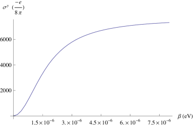
Figure 1: (Color online) $\overline{\sigma^{y}}$ as a function of $\beta$. The parameters are given by $V=0$, $\alpha_{+}=5.5\times 10^{-14}\textrm{eV~{}m}$, $\alpha_{-}=0.45\times 10^{-14}\textrm{eV~{}m}$, $\mu=0.1~{}\textrm{eV}$, $\tau=660~{}\textrm{fs}$ and the effective mass $m=0.065~{}m_{0}$ as in GaAs with $m_{0}$ being the mass of the free electron.

We plot $\overline{\sigma^{y}}$ as a function of the applied gate voltage $V$ with different $\alpha_{-}$ and momentum relaxation time in Fig. 2. It is shown that $\overline{\sigma^{y}}$ is an even function of the gate voltage. For small $\alpha_{-}$, a peak in $\overline{\sigma^{y}}$ appears around $V=0$. As $\alpha_{-}$ increases, this peak begins to split and its height increases. Additionally, the nonmagnetic impurities tend to suppress these peaks, as shown in Fig. 2(b) where the momentum relaxation time is a tenth part of that in Fig. 2(a).

Figure 3 shows the contour-plot projections of $\overline{\sigma^{y}}$ which are plotted as a function of both the gate voltage and $\alpha_{-}$. These figures indicate that the resonant peaks in $\overline{\sigma^{y}}$ begin to converge as $\alpha_{-}$ decreases.

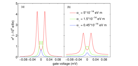
Figure 2: (Color online) Tunneling spin conductivities $\overline{\sigma^{y}}$ are plotted as functions of the gate voltage $V$ with different values of $\alpha_{-}$ given in the legend. The tunneling strength is $\beta=5\times 10^{-6}\textrm{eV}$, the momentum relaxation time are $\tau=660\textrm{fs}$ in panel (a) and $\tau=66\textrm{fs}$ in panel (b) while the other parameters are the same as those in Fig. 1.

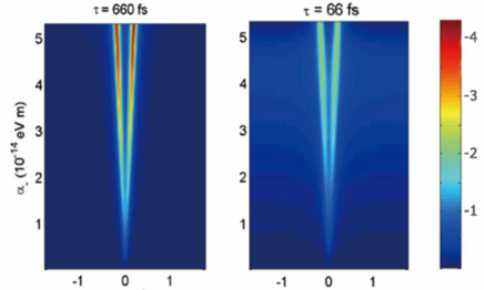
Figure 3: (Color online) Contour plot of $\overline{\sigma^{y}}$ which is a function of both the gate voltage and $\alpha_{-}$. The color bar represents the value of $\overline{\sigma^{y}}$ in unit of $10^{4}e/8\pi$.

IV Tunneling spin current asymmetrical to gate voltage

In realistic samples, the strengthes of impurity potentials in those two layers may not happen to be identical. We thus introduce $u_{\!f}$ and $u_{b}$ to denote the strengthes of impurity potentials in the front and back layers, respectively. Accordingly, the interaction between electrons and impurities is given by

$$\hat{V}_{\text{im}}=\sum_{i}\delta(\mathbf{r}-\mathbf{R}_{i})\left(\begin{array}[]{cc}u_{\!f}&0\\ 0&u_{b}\\ \end{array}\right)\otimes I.$$ (19)

Note that the unit matrix in the layer space is no longer appropriate in the present case. This implies that the line which refers to the impurity potential in the Feynman diagram (see Fig. 4) represents a matrix $\textrm{diag}(u_{f}/A,u_{b}/A)$ rather than a number $u/A$.

Figure 4: The first order Feynman diagram in the expansion of the impurity-averaged Green’s function where the momentum is conserved at the vertex. The vector refers to the free Green’s function. And the dotted line represents the impurity potential which is in the matrix form for the unequal strengthes of impurity potentials between layers.

Accordingly, the Dyson equation for $\overline{G^{R}}$ is then written as

$$\overline{G^{R}}(\mathbf{k},\omega)=G^{R}_{0}(\mathbf{k},\omega)+G^{R}_{0}(\mathbf{k},\omega)N\Big{[}\left(\begin{array}[]{cc}\frac{u_{\!f}}{A}&0\\ 0&\frac{u_{b}}{A}\\ \end{array}\right)\hskip 8.53581pt$$ (22)

$$+\sum_{\mathbf{q}}\left(\begin{array}[]{cc}\frac{u_{\!f}}{A}&0\\ 0&\frac{u_{b}}{A}\\ \end{array}\right)\overline{G^{R}}(\mathbf{q},\omega)\left(\begin{array}[]{cc}\frac{u_{\!f}}{A}&0\\ 0&\frac{u_{b}}{A}\\ \end{array}\right)\Bigr{]}\overline{G^{R}}(\mathbf{k},\omega).$$ (27)

We obtain a self-consistent solution for the above equation

$$\overline{G^{R}_{(ch)}}=\left(\begin{array}[]{cccc}R_{11}&R_{\!f}&0&0\\ R_{\!f}&R_{22}&0&0\\ 0&0&R_{33}&R_{b}\\ 0&0&R_{b}&R_{44}\\ \end{array}\right),$$ (32)

with nonvanishing off-diagonal elements even in the chiral representation. The explicit expressions for those matrix elements are given in the Appendix. The momentum relaxation time for the front and back layers are simply given by $\tau_{\!f}=(2\pi u^{2}_{\!f}n_{\text{im}}N_{F})^{-1}$ and $\tau_{b}=(2\pi u^{2}_{b}n_{\text{im}}N_{F})^{-1}$, respectively.

The difference between the strengthes of impurity potentials in two layers not only modifies the diagonal elements of $\overline{G^{R}_{(ch)}}$ but also requires the appearance of off-diagonal elements inevitably. Now the contributions to $\overline{\sigma^{y}}$ by the diagonal elements can be directly obtained by replacing $g_{i}$ and $a_{i}$, respectively, by $R_{ii}$ and $A_{ii}$ in Eq. (III) and Eq. (A). Here $A_{ii}=R_{ii}^{*}$ denote the diagonal elements of the averaged advanced Green’s function in the chiral representation. And the contributions to $\overline{\sigma^{y}_{0}}$ given by the off-diagonal elements reads

$$\overline{\sigma^{y}_{0,d}}=-2\beta\sum_{\mathbf{k}}\sin^{2}\!\varphi~{}\textrm{Im}\Bigl{[}\hskip 133.72795pt$$

$$\times R_{\textrm{f}}((A_{11}\!-\!A_{22})(\frac{k}{m}\!-\!\alpha_{+})+(A_{11}\!+\!A_{22})\frac{\alpha_{-}(eV\!-\!\alpha_{-}k)}{\lambda_{12}}$$

$$+(A_{33}\!+\!A_{44})\frac{eV\alpha_{-}\!+\!\alpha^{2}_{+}k}{\lambda_{12}}-(A_{33}\!-\!A_{44})\frac{\alpha_{+}\lambda_{34}}{\lambda_{12}})\hskip 28.45274pt$$

$$-R_{\textrm{b}}((A_{33}\!-\!A_{44})(\frac{k}{m}\!+\!\alpha_{+})-(A_{33}\!+\!A_{44})\frac{\alpha_{-}(eV\!+\!\alpha_{-}k)}{\lambda_{34}}$$

$$-(A_{11}\!+\!A_{22})\frac{eV\alpha_{-}\!-\!\alpha^{2}_{+}k}{\lambda_{34}}+(A_{11}\!-\!A_{22})\frac{\alpha_{+}\lambda_{12}}{\lambda_{34}})\Bigr{]}.\hskip 21.33955pt$$

The transfer matrix equation for the vertex $\mathcal{J}^{y}$ is also modified as

$$\mathcal{J}^{y}=N\sum_{\mathbf{q}}\left(\begin{array}[]{cc}\frac{u_{\!f}}{A}&0\\ 0&\frac{u_{b}}{A}\\ \end{array}\right)\overline{G^{A}}(\mathbf{q})\hskip 39.83385pt$$ (35)

$$\times(\hat{j}^{y}_{z}(\mathbf{q})+\mathcal{J}^{y})~{}\overline{G^{R}}(\mathbf{q})\left(\begin{array}[]{cc}\frac{u_{\!f}}{A}&0\\ 0&\frac{u_{b}}{A}\\ \end{array}\right).$$ (38)

And the terms in $\overline{\sigma^{y}_{L}}$ given by the off-diagonal elements is written out in the Appendix.

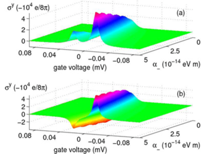
Figure 5: (Color online) $\overline{\sigma^{y}}$ as function of $V$ and $\alpha_{-}$. The relaxation-time differences are $\Delta\tau=8\times 10^{-5}$ in panel (a) and $\Delta\tau=5\times 10^{-4}$ in panel (b) with $\tau_{\textrm{b}}=660~{}\textrm{fs}$.

The influence of the difference of impurity potentials on the tunneling spin conductivity can be observed in Fig. 5. Here we introduce the difference in relaxation times $\Delta\tau=(\tau_{\!f}-\tau_{b})/\tau_{b}$ which is taken to be $8\times 10^{-5}$ and $5\times 10^{-4}$ in Fig. 5(a) and Fig. 5(b), respectively. As the difference $\Delta\tau$ increases, one of the resonant peak in $\overline{\sigma^{y}}$ tends to be suppressed and finally it becomes a valley.

Figure 5 shows that the variation of the strengthes of impurity potentials between layers leads to the asymmetric dependence of the TSC on the gate voltage when the in-plane driven electric field is fixed. This unilateral conduction feature makes the bilayer system with different strengthes of impurity potentials a candidate for the realization of spin diode.

V Summary

We have studied the coherent TSC in the bilayer system with spin-orbit coupling. We first revisited the definition of the tunneling charge current with the help of continuity-like equations in the bilayer system since the tunneling between layers causes the nonconservation of the density in each layer. In additional to the conventional contribution, the tunneling current contains those related to the overlap of wavefunctions for different layers. This is intuitional for us to define the coherent TSC. We showed that the contributions of the wavefunction overlaps for states with spin parallel and anti-parallel to reference axis have opposite signs. Unlike the conventional tunneling Hamiltonian approach, the tunneling strength in our study is not necessarily week since it is treated as a part of the unperturbed Hamiltonian. In the light that only a gate voltage can not induce a nonvanishing result, we studied TSC in response to an in-plane electric field. The spin conductivity was calculated in terms of Kubo formula by taking account of nonmagnetic impurities. We firstly investigated twin-layer systems and then considered the effect caused by the difference between the strengths of impurity potentials in different layers. Meanwhile, we developed the techniques dealing with the impurity-averaged Green’s function in the bilayer system. We showed that there must exist nonvanishing off-diagonal elements in the averaged Green’s function even in the chiral representation if the strengthes of impurity potentials in two layers is different. Sharp cusps in the tunneling spin conductivity appear near the null voltage and are suppressed by the impurities. We found that if the strength of impurity potential in one layer is different from that in the other layer, the TSC exhibits the asymmetrical feature with respect to the gate voltage. This reveals that the spin diode can also be realized in the bilayer system with different strengthes of impurity potentials in different layers.

Appendix A Expressions for some coefficients and the matrices

The concrete expressions for the matrix elements of the averaged retarded Green’s function is given by

$$R_{11} = \frac{\omega-\varepsilon_{2}-w_{+}-\frac{eV-\alpha_{-}k}{\lambda_{12}}w_{-}}{(\omega-\varepsilon_{1})(\omega-\varepsilon_{2})-w_{+}(2\omega-\varepsilon_{1}-\varepsilon_{2})+(\omega_{+}+\omega_{-})(\omega_{+}-\omega_{-})-2\omega_{-}(eV-\alpha_{-}k)},$$

$$R_{22} = \frac{\omega-\varepsilon_{1}-w_{+}+\frac{eV-\alpha_{-}k}{\lambda_{12}}w_{-}}{(\omega-\varepsilon_{1})(\omega-\varepsilon_{2})-w_{+}(2\omega-\varepsilon_{1}-\varepsilon_{2})+(\omega_{+}+\omega_{-})(\omega_{+}-\omega_{-})-2\omega_{-}(eV-\alpha_{-}k)},$$

$$R_{33} = \frac{\omega-\varepsilon_{4}-w_{+}-\frac{eV+\alpha_{-}k}{\lambda_{34}}w_{-}}{(\omega-\varepsilon_{3})(\omega-\varepsilon_{4})-w_{+}(2\omega-\varepsilon_{3}-\varepsilon_{4})+(\omega_{+}+\omega_{-})(\omega_{+}-\omega_{-})-2\omega_{-}(eV+\alpha_{-}k)},$$

$$R_{44} = \frac{\omega-\varepsilon_{3}-w_{+}+\frac{eV+\alpha_{-}k}{\lambda_{34}}w_{-}}{(\omega-\varepsilon_{3})(\omega-\varepsilon_{4})-w_{+}(2\omega-\varepsilon_{3}-\varepsilon_{4})+(\omega_{+}+\omega_{-})(\omega_{+}-\omega_{-})-2\omega_{-}(eV+\alpha_{-}k)},$$

$$R_{\textrm{f}} = -\frac{\frac{\beta}{\lambda_{12}}w_{-}}{(\omega-\varepsilon_{1})(\omega-\varepsilon_{2})-w_{+}(2\omega-\varepsilon_{1}-\varepsilon_{2})+(\omega_{+}+\omega_{-})(\omega_{+}-\omega_{-})-2\omega_{-}(eV-\alpha_{-}k)},$$

$$R_{\textrm{b}} = -\frac{\frac{\beta}{\lambda_{34}}w_{-}}{(\omega-\varepsilon_{3})(\omega-\varepsilon_{4})-w_{+}(2\omega-\varepsilon_{3}-\varepsilon_{4})+(\omega_{+}+\omega_{-})(\omega_{+}-\omega_{-})-2\omega_{-}(eV+\alpha_{-}k)},$$ (39)

with $w_{\pm}=\frac{1}{2}((u_{\!f}\pm u_{b})n_{\text{im}}-\frac{i}{\tau_{\pm}})$ where $\tau_{\pm}=\frac{1}{2}(\tau_{\!f}-\tau_{b})$ are introduced.

When the strengthes of impurities are equal in the two layers, the vertex correction to $\overline{\sigma^{y}}$ in terms of Green’s functions is given by

$$\overline{\sigma^{y}_{L}}=-\sum_{\mathbf{k}}\cos^{2}\!\varphi\Bigl{\{}\textrm{Re}\Bigl{[}(\frac{k}{m}\!-\!\alpha_{+}\!+\!\frac{\alpha_{-}(eV\!-\!\alpha_{-}k)}{\lambda_{12}})a_{1}g_{1}\!+\!(\frac{k}{m}\!+\!\alpha_{+}\!-\!\frac{\alpha_{-}(eV\!-\!\alpha_{-}k)}{\lambda_{12}})a_{2}g_{2}\!-\!\alpha_{+}(a_{1}\!+\!a_{2})(g_{3}\!+\!g_{4})\hskip 8.53581pt$$

$$-\!(\frac{k}{m}\!+\!\alpha_{+}\!-\!\frac{\alpha_{-}(eV\!+\!\alpha_{-}k)}{\lambda_{34}})a_{3}g_{3}\!-\!(\frac{k}{m}\!+\!\alpha_{+}\!+\!\frac{\alpha_{-}(eV\!+\!\alpha_{-}k)}{\lambda_{34}})a_{4}g_{4}\!-\!\alpha_{+}\frac{e^{2}V^{2}\!+\!\beta^{2}\!-\!\alpha^{2}_{-}k^{2}}{\lambda_{12}\lambda_{34}}(a_{1}\!-\!a_{2})(g_{3}\!-\!g_{4})\hskip 4.2679pt$$

$$+\alpha_{-}(\frac{eV-\alpha_{-}k}{\lambda_{12}}(a_{1}-a_{2})(g_{3}+g_{4})+\frac{eV+\alpha_{-}k}{\lambda_{34}}(a_{1}+a_{2})(g_{3}-g_{4}))\Bigr{]}\frac{i(J_{12}+J_{34})}{2}\hskip 105.27519pt$$

$$+\textrm{Re}\Bigl{[}-\frac{eV\!-\!\alpha_{-}k}{\lambda_{12}}((\frac{k}{m}\!-\!\alpha_{+}\!+\!\frac{\alpha_{-}(eV\!-\!\alpha_{-}k)}{\lambda_{12}})a_{1}g_{1}\!-\!(\frac{k}{m}\!-\!\alpha_{+}\!-\!\frac{\alpha_{-}(eV\!-\!\alpha_{-}k)}{\lambda_{12}})a_{2}g_{2}-\alpha_{+}(a_{1}\!-\!a_{2})(g_{3}\!+\!g_{4}))$$

$$\!+\!\frac{eV\!+\!\alpha_{-}k}{\lambda_{34}}((\frac{k}{m}\!+\!\alpha_{+}\!-\!\frac{\alpha_{-}(eV\!+\!\alpha_{-}k)}{\lambda_{34}})a_{3}g_{3}\!-\!(\frac{k}{m}\!+\!\alpha_{+}\!+\!\frac{\alpha_{-}(eV\!+\!\alpha_{-}k)}{\lambda_{34}})a_{4}g_{4}\!+\!\alpha_{+}(a_{1}\!+\!a_{2})(g_{3}\!-\!g_{4}))\hskip 29.87538pt$$

$$-\alpha_{-}(a_{1}\!+\!a_{2})(g_{3}\!+\!g_{4})\!-\!2\beta^{2}\alpha_{-}(\frac{a_{1}g_{2}}{\lambda^{2}_{12}}\!+\!\frac{a_{3}g_{4}}{\lambda^{2}_{34}})\!-\!\frac{\alpha_{-}(e^{2}V^{2}\!-\!\beta^{2}\!-\!\alpha^{2}_{-}k^{2})}{\lambda_{12}\lambda_{34}}(a_{1}\!-\!a_{2})(g_{3}\!-\!g_{4})\Bigr{]}\frac{i(J_{12}-J_{34})}{2}\hskip 28.45274pt$$

$$+\textrm{Re}\Bigl{[}-(\frac{k}{m}-\alpha_{+}+\frac{\alpha_{-}(eV-\alpha_{-}k)}{\lambda_{12}})\frac{a_{1}g_{1}}{\lambda_{12}}+(\frac{k}{m}-\alpha_{+}-\frac{\alpha_{-}(eV-\alpha_{-}k)}{\lambda_{12}})\frac{a_{2}g_{2}}{\lambda_{12}}+\frac{\alpha_{+}}{\lambda_{12}}(a_{1}-a_{2})(g_{3}+g_{4})\hskip 12.80373pt$$

$$+(\frac{k}{m}+\alpha_{+}-\frac{\alpha_{-}(eV+\alpha_{-}k)}{\lambda_{34}})\frac{a_{3}g_{3}}{\lambda_{34}}-(\frac{k}{m}+\alpha_{+}+\frac{\alpha_{-}(eV+\alpha_{-}k)}{\lambda_{34}})\frac{a_{4}g_{4}}{\lambda_{34}}+\frac{\alpha_{+}}{\lambda_{34}}(a_{1}+a_{2})(g_{3}-g_{4})\hskip 36.98857pt$$

$$+2\alpha_{-}(\frac{eV-\alpha_{-}k}{\lambda^{2}_{12}}a_{1}g_{2}+\frac{eV+\alpha_{-}k}{\lambda^{2}_{34}}a_{3}g_{4}-\frac{eV}{\lambda_{12}\lambda_{34}}(a_{1}-a_{2})(g_{3}-g_{4}))\Bigr{]}\frac{i\beta(J_{14}+J_{32})}{2}\hskip 91.04881pt$$

$$+\textrm{Im}\Bigl{[}\frac{a_{1}g_{2}}{\lambda_{12}}\!-\!\frac{(a_{3}\!+\!a_{4})(g_{1}\!-\!g_{2})}{2\lambda_{12}}\!+\!\frac{a_{3}g_{4}}{\lambda_{34}}\!-\!\frac{(a_{1}+a_{2})(g_{3}-g_{4})}{2\lambda_{34}}\!-\!\frac{\alpha_{+}k}{\lambda_{12}\lambda_{34}}(a_{1}\!-\!a_{2})(g_{3}\!-\!g_{4})\Bigr{]}\alpha_{-}\beta(J_{14}-J_{32})\Bigr{\}},\hskip 11.38109pt$$ (40)

where $J_{12},J_{14},J_{32},J_{34}$ are the matrix elements of the vertex $\mathcal{J}^{y}$ which can be obtained by solving Eq. (16).

The difference of strengthes of impurity potentials in each layer brings the off-diagonal elements to the Green’s function in the chiral representation. The corresponding contribution to the vertex correction of the conductivity is given by

$$\overline{\sigma^{y}_{L,d}}=-\sum_{\mathbf{k}}\cos^{2}\!\varphi\Bigl{\{}\textrm{Re}\Bigl{[}A_{\textrm{f}}R_{\textrm{f}}(\frac{k}{m}-\alpha_{+})-A_{\textrm{b}}R_{\textrm{b}}(\frac{k}{m}+\alpha_{+})+\beta\alpha_{-}(R_{11}+R_{22}+R_{33}+R_{44})(\frac{A_{\textrm{f}}}{\lambda_{12}}+\frac{A_{\textrm{b}}}{\lambda_{34}})\hskip 39.83385pt$$

$$-\frac{2\alpha_{+}}{\lambda_{12}\lambda_{34}}(A_{\textrm{f}}R_{\textrm{b}}(e^{2}V^{2}+\beta^{2}-\alpha^{2}_{-}k^{2})+(A_{\textrm{f}}(R_{33}-R_{44})-A_{\textrm{b}}(R_{11}-R_{22}))\beta\alpha_{-}k)\Bigr{]}i(J_{12}+J_{34})\hskip 65.44133pt$$

$$+\textrm{Re}\Bigl{[}-\frac{\beta}{\lambda_{12}}A_{\textrm{f}}((R_{11}+R_{22})(\frac{k}{m}-\alpha_{+})-(R_{33}+R_{44})\alpha_{+})+\frac{\beta}{\lambda_{34}}A_{\textrm{b}}((R_{33}+R_{44})(\frac{k}{m}+\alpha_{+})+(R_{11}+R_{22})\alpha_{+})$$

$$+\frac{2\alpha_{-}}{\lambda_{12}}(A_{\textrm{f}}R_{\textrm{b}}\frac{e^{2}V^{2}-\beta^{2}-\alpha^{2}_{-}k^{2}}{\lambda_{34}}-(A_{\textrm{f}}(R_{33}-R_{44})+A_{\textrm{b}}(R_{11}-R_{22}))\frac{eV\beta}{\lambda_{34}}+A_{\textrm{f}}R_{\textrm{f}}\frac{(eV-\alpha_{-}k)^{2}-\beta^{2}}{2\lambda_{12}})\hskip 27.0301pt$$

$$-A_{\textrm{f}}(R_{11}\!-\!R_{22})\frac{2\alpha_{-}\beta(eV\!-\!\alpha_{-}k)}{\lambda^{2}_{12}}+A_{\textrm{b}}R_{\textrm{b}}\frac{\alpha_{-}((eV\!+\!\alpha_{-}k)^{2}\!-\!\beta^{2})}{\lambda^{2}_{34}}\!-\!A_{\textrm{b}}(R_{33}\!-\!R_{44})\frac{2\beta(eV\!+\!\alpha_{-}k)}{\lambda^{2}_{34}}\Bigr{]}i(J_{12}-J_{34})\hskip 2.84526pt$$

$$+\textrm{Re}\Bigl{[}\frac{eV\!-\!\alpha_{-}k}{\lambda_{12}}A_{\textrm{f}}((R_{11}\!+\!R_{22})(\frac{k}{m}\!-\!\alpha_{+})\!-\!\alpha_{+}(R_{33}\!+\!R_{44})\!+\!R_{\textrm{f}}\frac{2\alpha_{-}\beta}{\lambda_{12}})\!+\!\alpha_{-}A_{\textrm{f}}(R_{11}\!-\!R_{22})\frac{(eV\!-\!\alpha_{-}k)^{2}\!-\!\beta^{2}}{\lambda^{2}_{12}}\hskip 17.07164pt$$

$$+\frac{eV\!+\!\alpha_{-}k}{\lambda_{34}}A_{\textrm{b}}((R_{33}\!+\!R_{44})(\frac{k}{m}\!+\!\alpha_{+})\!-\!\alpha_{+}(R_{11}\!+\!R_{22})\!+\!R_{\textrm{b}}\frac{2\alpha_{-}\beta}{\lambda_{34}})\!+\!\alpha_{-}A_{\textrm{b}}(R_{33}\!-\!R_{44})\frac{(eV\!+\!\alpha_{-}k)^{2}\!-\!\beta^{2}}{\lambda^{2}_{34}}\hskip 27.0301pt$$

$$+\frac{\alpha_{-}}{\lambda_{12}\lambda_{34}}(4eV\beta A_{\textrm{f}}R_{\textrm{b}}+(A_{\textrm{f}}(R_{33}-R_{44})+A_{\textrm{b}}(R_{11}-R_{22}))(e^{2}V^{2}-\beta^{2}-\alpha^{2}_{-}k^{2}))\Bigr{]}i(J_{14}+J_{32})\hskip 66.86397pt$$

$$-\textrm{Im}\Bigl{[}\frac{\alpha_{+}}{\lambda_{12}\lambda_{34}}(4\beta\alpha_{-}kA_{\textrm{f}}R_{\textrm{b}}\!-\!(A_{\textrm{f}}(R_{33}\!-\!R_{44})\!-\!(A_{11}\!-\!A_{22})R_{\textrm{b}})(e^{2}V^{2}\!+\!\beta^{2}\!-\!\alpha^{2}_{-}k^{2}))\!+\!A_{\textrm{f}}(R_{11}\!-\!R_{22})(\frac{k}{m}\!-\!\alpha_{+})\hskip 11.38109pt$$

$$+\alpha_{-}(R_{11}\!+\!R_{22}\!+\!R_{33}\!+\!R_{44})(\frac{(eV\!-\!\alpha_{-}k)A_{\textrm{f}}}{\lambda_{12}}\!+\!\frac{(eV\!+\!\alpha_{-}k)A_{\textrm{b}}}{\lambda_{34}})\!-\!A_{\textrm{b}}(R_{33}\!-\!R_{44})(\frac{k}{m}\!+\!\alpha_{+})\Bigr{]}(J_{14}-J_{32})\Bigr{\}}.\hskip 29.87538pt$$ (41)

References

• (1) R. Fitzgerald, Phys. Today 55, No. 6, 14 (2002).
• (2) J. Q. You and F. Nori, Phys. Today 58, No. 11, 42 (2005).
• (3) M. I. Dyakonov and V. I. Perel, JETP Lett. 13, 467 (1971).
• (4) S. A. Wolf, D. D. Awschalom, R. A. Buhrman, J. M. Daughton, S. von Molnar, M. L. Roukes, A. Y. Chtchelkanova, and D. M. Tresger, Science 294, 1488 (2001).
• (5) I. Zutic, J. Fabian, and S. DasSarma, Rev. Mod. Phys. 76, 323 (2004).
• (6) Mahn-Soo Choi, C. Bruder, and D. Loss, Phys. Rev. B 62, 13569 (2000).
• (7) M. S. Grønsleth, J. Linder, J.-M. Børven, and A. Sudbø, Phys. Rev. Lett. 97, 147002 (2006).
• (8) Erhai Zhao and J. A. Sauls, Phys. Rev. Lett. 98, 206601 (2007).
• (9) Yu-Li Lee and Yu-Wen Lee, Phys. Rev. B 68, 184413 (2003).
• (10) I. B. Spielman, J. P. Eisenstein, L. N. Pfeiffer, and K. W. West, Phys. Rev. Lett. 84, 5808 (2000).
• (11) P. Q. Jin and Y. Q. Li, Phys. Rev. B 76, 235311 (2007).
• (12) M. H. Cohen, L. M. Falicov and J. C. Phillips, Phys. Rev. Lett. 8, 316 (1962).
• (13) R. E. Prange, Phys. Rev. 131, 1083 (1963).
• (14) A. Zawadowski, Phys. Rev. 163, 341 (1967).
• (15) C. Caroli, R. Combescot, D. Lederer, P. Nozi$\grave{e}$res, and D. Saint-James, Phys. Rev. B 12, 3977 (1975).
• (16) P. Q. Jin, Y. Q. Li, and F. C. Zhang, J. Phys. A 39, 7115 (2006); ibid., Phys. Rev. B 77, 155304 (2008).
• (17) S. Murakami, N. Nagaosa, and S. C. Zhang, Science 301, 1348 (2003); J. Sinova, D. Culcer, Q. Niu, N. A. Sinitsyn, T. Jungwirth, and A. H. MacDonald, Phys. Rev. Lett. 92, 126603 (2004).
• (18) G. D. Mahan, Many-Particle Physics (Plenum Press, New York, 2000).
• (19) J. I. Inoue, G. E. W. Bauer, and L. W. Molenkamp, Phys. Rev. B 67, 033104 (2003); ibid. 70, 041303(R) (2004).
• (20) E. G. Mishchenko, A. V. Shytov, and B. I. Halperin, Phys. Rev. Lett. 93, 226602 (2004).
• (21) Ol’ga V. Dimitrova, Phys. Rev. B 71, 245327 (2005).
• (22) H.-A. Engel, E. I. Rashba, and B. I. Halperin, Handbook of Magnetism and Advanced Magnetic Materials (Wiley, New York,2006), Vol. V.
• (23) J. I. Inoue, T. Kato, Y. Ishikawa, H. Itoh, G. E. W. Bauer, and L. W. Molenkamp, Phys. Rev. Lett. 97, 046604 (2006).
• (24) P. Wang, Y. Q. Li, and X. Zhao, Phys. Rev. B 75, 075326 (2007).
• (25) H. Haug and A.-P. Jauho, Quantum Kinetics in Transport and Optics of Semiconductors (Springer-Verlag, Berlin, 1996).
• (26) A. A. Abrikosov, L. P. Gorkov and I. E. Dzyaloshinski, Methods of Quantum Field Theory in Statistical Physics (Dover, New York, 1975).