A Theoretical Model of Chaotic Attractor
in Tumor Growth and Metastasis

Abstract

This paper proposes a novel chaotic reaction-diffusion model of cellular tumor growth and metastasis. The model is based on the multiscale diffusion cancer-invasion model (MDCM) and formulated by introducing strong nonlinear coupling into the MDCM. The new model exhibits temporal chaotic behavior (which resembles the classical Lorenz strange attractor) and yet retains all the characteristics of the MDCM diffusion model. It mathematically describes both the processes of carcinogenesis and metastasis, as well as the sensitive dependence of cancer evolution on initial conditions and parameters. On the basis of this chaotic tumor-growth model, a generic concept of carcinogenesis and metastasis is formulated.

Keywords: reaction-diffusion tumor growth model, chaotic attractor, sensitive dependence on initial tumor characteristics

1 Introduction

Cancer is one of the main causes of morbidity and mortality in the world. There are several different stages in the growth of a tumor before it becomes so large that it causes the patient to die or reduces permanently their quality of life. Developed countries are investing large sums of money into cancer research in order to find cures and improve existing treatments. In comparison to molecular biology, cell biology, and drug delivery research, mathematics has so far contributed relatively little to the area [1].

A number of mathematical models of avascular (solid) tumor growth were reviewed in [2]. These were generally divided into continuum cell population models described by diffusion partial differential equations (PDEs) of continuum mechanics [3, 4] combined with chemical kinetics, and discrete cell population models described by ordinary differential equations (ODEs).

On the other hand, in many biological systems it is possible to empirically demonstrate the presence of attractors that operate starting from different initial conditions [5]. Some of these attractors are points, some are closed curves, while the others have non–integer, fractal dimension and are termed “strange attractors” [6]. It has been proposed that a prerequisite for proper simulating tumor growth by computer is to establish whether typical tumor growth patterns are fractal. The fractal dimension of tumor outlines was empirically determined using the box-counting method [7]. In particular, fractal analysis of a breast carcinoma was performed using a morphometric method, which is the box-counting method applied to the mammogram as well as to the histologic section of a breast carcinoma [8].

If tumor growth is chaotic, this could explain the unreliability of treatment and prediction of tumor evolution. More importantly, if chaos is established, this could be used to adjust strategies for fighting cancer. Treatment could include some form of chaos control and/or anti-control.

In this paper, a plausible chaotic diffusion model of tumor growth and metastasis is presented. The approach is a combination of theoretical modelling and empirical search.

2 A multiscale diffusion cancer-invasion model

Recently, a multiscale diffusion cancer-invasion model (MDCM) was presented in [9, 10, 11, 12, 13, 14, 15, 16, 17], which considers cellular and microenvironmental factors simultaneously and interactively. The model was classified as hybrid, since a continuum deterministic model (based on a system of reaction–diffusion chemotaxis equations) controls the chemical and extracellular matrix (ECM) kinetics and a discrete cellular automata-like model (based on a biased random-walk model) controls the cell migration and interaction. The interactions of the tumor cells, matrix–metalloproteinases (MMs), matrix-degradative enzymes (MDEs) and oxygen are described by the four coupled rate PDEs:

$$\frac{\partial n}{\partial t} = D_{n}\nabla^{2}n-\chi\nabla\cdot(n\nabla f),$$ (1)

$$\frac{\partial f}{\partial t} = -\delta mf,$$ (2)

$$\frac{\partial m}{\partial t} = D_{m}\nabla^{2}m+\mu n-\lambda m,$$ (3)

$$\frac{\partial c}{\partial t} = D_{c}\nabla^{2}c+\beta f-\gamma n-\alpha c,$$ (4)

where $n$ denotes the tumor cell density, $f$ is the MM–concentration, $m$ corresponds to the MDE–concentration, and $c$ denotes the oxygen concentration. The four variables, $n,m,f,c$, are all functions of the 3-dimensional spatial variable $x$ and time $t$. All equations represent diffusion except (2), which shows only temporal evolution of the MM–concentration coupled to the MDE–concentration. $D_{n}$ is the tumor cell coefficient, $D_{m}$ is the MDE coefficient and $D_{c}>0$ is the oxygen diffusion coefficient, while $\chi,\mu$, $\lambda$, $\delta$, $\alpha$, $\gamma$, $\beta$ are positive constants. The other terms respectively denote:

$\chi\nabla\cdot(n\nabla f)-$haptotaxis;

$\mu N-$production of MDE by tumor cell;

$\lambda m-$decay of MDE;

$\delta mf-$degradation of MM by MDE;

$\alpha c-$natural decay of oxygen;

$\gamma n-$oxygen uptake; and

$\beta f-$production of oxygen by MM.

Because of its hybrid nature (cells treated as discrete entities and microenvironmental parameters treated as continuous concentrations), the 4–dimensional (4D) model (1)–(4) can be directly linked to experimental measurements of those cellular and microenvironmental parameters recognized by cancer biologists as important in cancer invasion. Furthermore, the fundamental unit of the model is the cell, and the complex collective behavior of the tumor emerges as a consequence of interactions between factors influencing the life cycle and movement of individual cells [9, 11, 12, 15, 16, 17].

In order to use realistic parameter values, the system of rate equations (1)–(4) was non-dimensionalised. The resulting 4D scaled system of rate PDEs [11] is given by

$$\frac{\partial n}{\partial t} = d_{n}\nabla^{2}n-\rho\nabla\cdot(n\nabla f),$$ (5)

$$\frac{\partial f}{\partial t} = -\eta mf,$$ (6)

$$\frac{\partial m}{\partial t} = d_{m}\nabla^{2}m+\kappa n-\sigma m,$$ (7)

$$\frac{\partial c}{\partial t} = d_{c}\nabla^{2}c+\nu f-\omega n-\phi c.$$ (8)

In [11] the values of the non-dimensional parameters were given as:

$$d_{n}=0.0005,~{}~{}d_{m}=0.0005,~{}~{}d_{c}=0.5,~{}~{}\rho=0.01,~{}~{}\eta=50,$$

$$\kappa=1,~{}~{}\sigma=0,~{}~{}\nu=0.5,~{}~{}\omega=0.57,~{}~{}\phi=0.025.$$ (9)

The 4D hybrid PDE–model (1)–(4) can be seen as a special case of a general multi–phase tumor growth PDE ([2] equation (12)),

$$\frac{\partial\Phi_{i}}{\partial t}+\nabla\cdot(\mathbf{v}_{i}\Phi_{i})=\nabla\cdot(D_{i}\Phi_{i})+\lambda_{i}(\Phi_{i},C_{i})-\mu_{i}(\Phi_{i},C_{i}),$$ (10)

where for phase $i$, $\Phi_{i}$ is the volume fraction ($\sum_{i}\Phi_{i}=1$), $\mathbf{v}_{i}$ is the velocity, $D_{i}$ is the random motility or diffusion, $\lambda_{i}(\Phi_{i},C_{i})$ is the chemical and phase dependent production, and $\mu_{i}(\Phi_{i},C_{i})$ is the chemical and phase dependent degradation/death. The multi-phase model (10) has been derived from the basic conservation equations for the different chemical species,

$$\frac{\partial C_{i}}{\partial t}+\nabla\cdot\mathbf{N}_{i}=P_{i},$$

where $C_{i}$ are the concentrations of the chemical species, subindex $a$ for oxygen, $b$ for glucose, $c$ for lactate ion, $d$ for carbon dioxide, $e$ for bicarbonate ion, $f$ for chloride ion, and $g$ for hydrogen ion concentration; $\mathbf{N}_{i}$ is the flux of each of the chemical species inside the tumor spheroid; and $P_{i}$ is the net rate of consumption/production of the chemical species both by tumor cells and due to the chemical reactions with other species.

In this paper we will search for a temporal 3D cancer chaotic attractor ‘buried’ within the 4D hybrid spatio-temporal model (1)–(4).

3 A chaotic multi-scale cancer-invasion model

From the non–dimensional spatio-temporal AC model (5)–(8), discretization was performed by neglecting all the spatial derivatives resulting in the following simple 4D temporal dynamical system.

$$\dot{n} = 0,$$ (12)

$$\dot{f} = -\eta mf,$$ (13)

$$\dot{m} = \kappa n-\sigma m,$$ (14)

$$\dot{c} = \nu f-\omega n-\phi c.$$ (15)

When simulated, the temporal system (12)–(15) with the set of parameters (9) exhibits a virtually linear temporal behavior with almost no coupling between the four concentrations that have very different quantitative values (all phase plots between the four concentrations, not shown here, are virtually one-dimensional). To see if a modified version of the system (12)–(15) could lead to a chaotic description of tumor growth, four new parameters, $\alpha$, $\beta$, $\gamma$, and $\delta$ were introduced. The resulting model is

$$\dot{n} = 0,$$ (16)

$$\dot{f} = \alpha\eta(m-f),$$ (17)

$$\dot{m} = \beta\kappa n+f(\gamma-c)-m,$$ (18)

$$\dot{c} = \nu fm-\omega n-\delta\phi c.$$ (19)

The introduction of the parameters $(\alpha,\beta,\gamma,\delta)$ was motivated by the fact that tumor cell shape (see Figures 6 and 7) represents a visual manifestation of an underlying balance of forces and chemical reactions [32]. Specifically, the parameters represent the following quantities:

$\alpha~{}~{}{\rm=}$  tumor cell volume (proliferation/non-proliferation fraction),

$\beta~{}~{}{\rm=}$  glucose level,

$\gamma~{}~{}{\rm=}$  number of tumor cells,

$\delta~{}~{}{\rm=}$  diffusion from the surface (saturation level).

A tumor is composed of proliferating ($P$) and quiescent (or non-proliferating) ($Q$) cells. Tumor cells shift from class $P$ to class $Q$ as the tumor grows in size [33]. Model dependence on the ratio of proliferation to non-proliferation is introduced via the first parameter, $\alpha$. The discretization of equation (5) leads to cell density being modelled as a constant in equation (12). Accordingly, cell density does not play a role in the dynamics. In (16)–(19) the cell density is re-introduced into the dynamics via the cell number, $\gamma$. The importance of introducing $\gamma$ also appears in connection with the cyclin-dependent kinase (Cdk) inhibitor p27, the level and activity of which increase in response to cell density. Levels and activity of Cdk inhibitor p27 also increase with differentiation following loss of adhesion to the ECM [29].

The ability to estimate the growth pattern of an individual tumor cell type on the basis of morphological measurements should have general applicability in cellular investigations, cell–growth kinetics, cell transformation and morphogenesis [34].

Cell spreading alone is conducive to proliferation and increases in DNA synthesis, indicating that cell morphology is a critical determinant of cell function, at least in the presence of optimal growth factors and extracellular matrix (ECM) binding [35]. In many cells, the changes in morphology can stimulate cell proliferation through integrin-mediated signaling, indicating that cell shape may govern how individual cells will respond to chemical signals [36].

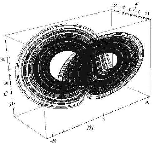
Figure 1: A 3D Lorenz-like chaotic attractor (see [22, 23]) from the modified tumor growth model (16)-(19). The attractor effectively couples the MM–concentration $f$, the MDE–concentration $m$, and the oxygen concentration $c$ in a mask–like fashion.

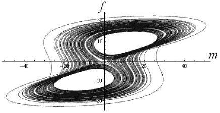
Figure 2: The $m-f$ phase plot of the 3D attractor.

Parameters $(\alpha,\beta,\gamma,\delta)$, introduced in connection with cancer cells morphology and dynamics could also influence the very important factor chromatin associated with aggressive tumor phenotype and shorter patient survival time.

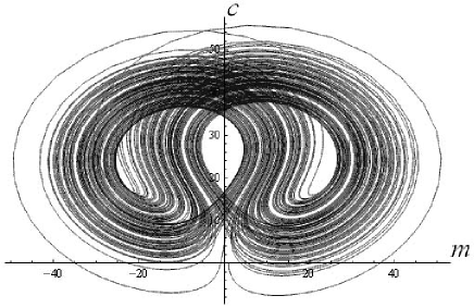
Figure 3: The $m-c$ phase plot of the 3D attractor.

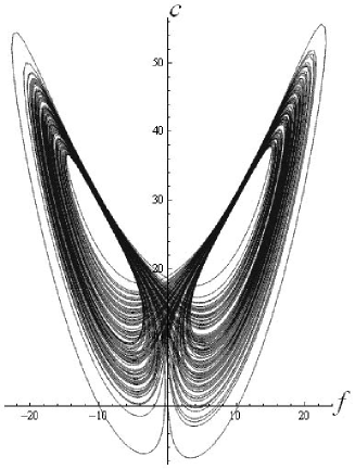
Figure 4: The $f-c$ phase plot of the 3D attractor.

For computations, the parameters were set to $\alpha$ = 0.06, $\beta$ = 0.05, $\gamma$ = 26.5 and $\delta$ = 40. Small variation of these chosen values would not affect the qualitative behavior of the new temporal model (16)–(19). Simulations of (16)–(19), using the same initial conditions and the same non-dimensional parameters as before, show chaotic behavior in the form of Lorenz-like strange attractor in the 3D ($f-m-c$) subspace of the full 4D ($n-f-m-c$) phase-space (Figures 1–4).

The spatio-temporal system of rate PDEs corresponding to the system in (15)–(18) provides the following multi-scale cancer invasion model.

$$\frac{\partial n}{\partial t} = d_{n}\nabla^{2}n-\rho\nabla\cdot(n\nabla f),$$ (20)

$$\frac{\partial f}{\partial t} = \alpha\eta(m-f),$$ (21)

$$\frac{\partial m}{\partial t} = d_{m}\nabla^{2}m+\kappa n-\sigma m,$$ (22)

$$\frac{\partial c}{\partial t} = d_{c}\nabla^{2}c+\nu f-\omega n-\phi c.$$ (23)

The new tumor–growth model (20)–(23) retains all the qualities of the original AC model (5)–(8) plus includes the temporal chaotic ‘butterfly’–attractor. This chaotic behavior may be a more realistic view on the tumor growth, including stochastic–like long–term unpredictability and uncontrollability, as well as sensitive dependence of a tumor growth on its initial conditions.

Based on the new tumor growth model (20)–(23), we have re-formulated the following generic concept of carcinogenesis and metastasis (see scheme on the following page). With the model of strongly coupled PDEs, remodelling of extracellular matrix (ECM) causes a whole process of the movement of invading cells with increased haptotaxis, and at the same time decreased enzyme productions level. This can alter chromatin structure, which plays an important role in initiating, propagating and terminating cellular response to DNA damage [28]. The effect of haptotaxis in the process of cells invading could be modelled with travelling-wave (Fisher) equation [18].

Extracellular matrix [ECM]

$\qquad\ \ \ \downarrow$

Carcinogenesis – nonlinearly coupled diffusion PDEs

$\ \ \ \downarrow\qquad\qquad\qquad\qquad\qquad\qquad\qquad\qquad\downarrow$

Mutation of p53 gene “Guardian of the Genome”        Subpopulations of tumor cells initiate tumor growth (cancer stem cells) [26]

$\qquad\ \ \ \downarrow$

$\begin{array}[]{c}\begin{tabular}[]{c}{ECM}\\ {Remodelling}\end{tabular}\\ \ \framebox{\ \begin{tabular}[]{c}ECM\\ primary tumor cell\\ $\framebox{\begin{tabular}[]{c}Extracellular\\ matrix\end{tabular} }$\\ $\downarrow$\\ $\framebox{\begin{tabular}[]{c}ECM\\ mutation cell\end{tabular} }$\end{tabular} }\\ \downarrow\text{escape}\\ \framebox{\begin{tabular}[]{c}Spontaneous\\ cell-cell fusion\end{tabular} }\\ \downarrow\\ \framebox{\begin{tabular}[]{c}Travelling through\\ the bloodstream\end{tabular} }\\ \downarrow\\ \framebox{\begin{tabular}[]{c}Stopping at a\\ distant site\end{tabular} }\\ \downarrow\\ \framebox{\begin{tabular}[]{c}Bone\\ marrow\end{tabular} }\end{array}$            $\begin{array}[]{c}\begin{tabular}[]{c}{Bone marrow:}\\ {Tumor--specific}\\ {premetastatic site}\\ {before metastasis}\\ ({pre-metastatic niches} \cite[cite]{[\@@bibref{}{Sleeman}{}{}]})\end{tabular}\\ \begin{array}[]{c}\framebox{\begin{tabular}[]{c}Bone marrow--derived\\ haematopoetic\\ progenitor cell express\end{tabular} }\\ \downarrow\end{array}\\ \framebox{\begin{tabular}[]{c}Vascular endotelial\\ growth--factor receptor 1\\ (VEGFR1) home\\ to tumor--specific\\ premetastatic site\end{tabular} }\\ \downarrow\\ \framebox{\begin{tabular}[]{c}Form cellar clusters\\ before the arrival\\ of tumor cells\end{tabular} }\\ \downarrow\\ \framebox{\begin{tabular}[]{c}VEGFR1 + cells\\ $\Rightarrow$ integrin $\alpha 4\beta 1$\\ -- adhesion molecule\\ which joins the cell\\ and ECM\end{tabular} }\\ \mathbf{Metastasis-Chaos}\end{array}$

Solution for cancer control:
Celular retraining of cancer stem cells [27] and/or activation of positive function of cyclin-dependent kinase inhibitor p27 [29] and/or decreased expression of SATB1 [30, 31]

The proposed model (20)–(23) describes chaotic behavior relevant to the invasion of cancer cells (see Figures 5 and 6). As devices for controlling metastasis/chaos we suggest the following processes: Cellular retraining of cancer stem cells and/or activation of positive function of cyclin-dependent kinase inhibitor p27 and/or decreased expression of SATB1, which is correlated with aggressive tumor phenotype in breast cancer and shorter patient survival time [27, 29, 30, 31].

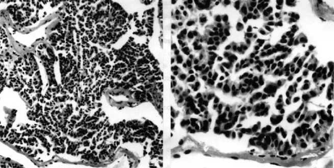
Figure 5: Carcinoma intraductale mamae: magnification at 160 $\times$ (left) and 420 $\times$ (right).

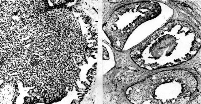
Figure 6: Carcinoma ductale in situ mamae with magnification at 80 $\times$ (left) and carcinoma comedo mamae with magnification at 420 $\times$ (right).

To connect the new parameters $(\alpha,\beta,\gamma,\delta)$ to the therapeutic regime we note the fact that significant factor of any therapy is tumor re-growth during the rest periods between therapy applications, which is again dependent on proliferation fraction dynamics $\alpha$ [33].

Also, the age of the tumor may translate to different levels of response to a standard therapy. As mentioned earlier, the number of cells, $\gamma$, is connected with the Cdk inhibitor p27, for which levels and activity increase in response with the cell density $\gamma$, differentiation following loss of adhesion to the ECM. Cdk inhibitor p27 regulates cell proliferation, cell motility and apoptosis and is the essential element for understanding transduction pathways in the regulation of normal and malignant cell proliferation as well as it is new hope for therapeutic intervention [29].

Introducing the parameter set $(\alpha,\beta,\gamma,\delta)$ into the model of tumor cell morphology and function could lead to insight into the relationship between these parameters and chromatin. By varying these parameters, it may be possible to predict situations that result in dangerous levels of chromatin. High levels of chromatin are associated with cancer metastasis and some of the most aggressive cancer types [30, 31].

The new temporal model (16)–(19) (as well as the corresponding spatio-temporal tumor-growth model (20)–(23)) is not sensitive to variation of the $(\alpha,\beta,\gamma,\delta)-$values, but is sensitive to their corresponding places in the equations.

4 Conclusion

A plausible chaotic multi-scale cancer-invasion model has been presented. The new model was formulated by introducing nonlinear coupling into the existing hybrid multiscale Anderson-Chaplain model. The new model describes chaotic behavior, as well as sensitive dependence of a tumor evolution on its initial conditions. On the basis of this chaotic tumor-growth model, a generic concept of carcinogenesis and metastasis was described. Effective cancer control is reflected in progressive reduction in cancer mortality [27]. The proposed model suggests a possible solution to carcinogenesis and metastasis, by combining mathematical modelling with latest medical discoveries.

Acknowledgment

The authors are grateful to Professor Nada Sljapic, MD, PhD, from the Medical School, University of Novi Sad, for expert advice and breast cancer slides.

The first author gratefully acknowledges the support of the Knowledge-Based Engineering Centre of University of South Australia.

5 Appendix

5.1 Vector Operators, PDEs and Diffusion Processes

5.1.1 The Hamilton operator $\nabla$

The core vector differential operator $\nabla$, called ‘nabla’ or ‘del’ operator, having properties analogous to those of ordinary vectors, invented by Sir William Rowan Hamilton (1805–1865), is defined in Cartesian ($x,y,z$)–coordinates as

$$\nabla=\frac{\partial}{\partial x}\mathbf{i}+\frac{\partial}{\partial y}\mathbf{j}+\frac{\partial}{\partial z}\mathbf{k},$$

where ($\mathbf{i,j,k}$) are the unit vectors of the coordinate axes ($x,y,z$), respectively.

Using Hamilton’s $\nabla-$operator, we can define the following three quantities (fundamental for vector calculus and its various applications):

The gradient.

Let $\phi(x,y,z)$ define a smooth scalar field. Then the gradient of $\phi$, denoted $\nabla\phi$ or grad $\phi$, is a vector field defined by

$$\text{{grad}}\,\phi=\nabla\phi=\frac{\partial\phi}{\partial x}\mathbf{i}+\frac{\partial\phi}{\partial y}\mathbf{j}+\frac{\partial\phi}{\partial z}\mathbf{k}.$$

The gradient $\text{{grad}}\,\phi$ is a vector field which points in the direction of the greatest rate of increase of the scalar field $\phi(x,y,z)$, and whose magnitude is the greatest rate of change.

The divergence.

Let $\mathbf{V}(x,y,z)=V_{1}\mathbf{i}+V_{2}\mathbf{j}+V_{3}\mathbf{k}$ define a smooth vector field. Then the divergence of $\mathbf{V}$, denoted $\nabla\cdot\mathbf{V}$ or div $\mathbf{V}$, is a scalar field defined by

$$\text{{div}}\,\mathbf{V}=\nabla\cdot\mathbf{V}=\frac{\partial V_{1}}{\partial x}+\frac{\partial V_{2}}{\partial y}+\frac{\partial V_{3}}{\partial z}.$$

The divergence $\text{{div}}\,\mathbf{V}(x,y,z)$ measures the magnitude of a vector field’s source or sink at a given point $(x,y,z)$. A vector field that has zero divergence everywhere is called solenoidal.

The curl.

If $\mathbf{V}(x,y,z)$ is a smooth vector field as above, then the curl or rotation of $\mathbf{V}$, denoted $\nabla\times\mathbf{V}$ or rot $\mathbf{V}$, is a vector field defined by the following determinant

$$\text{{rot}}\,\mathbf{V}=\nabla\times\mathbf{V}=\left|\begin{array}[]{ccc}\mathbf{i}&\mathbf{j}&\mathbf{k}\\ \frac{\partial}{\partial x}&\frac{\partial}{\partial y}&\frac{\partial}{\partial z}\\ V_{1}&V_{2}&V_{3}\end{array}\right|.$$

The curl shows a vector field’s rate of rotation, that is, the direction of the axis of rotation and the magnitude of the rotation. It can also be described as the circulation density. A vector field which has zero curl everywhere is called irrotational.

5.1.2 The Laplacian operator $\nabla^{2}$ and the fundamental PDEs

The Laplacian operator is the dot–product of the Hamilton operator by itself, that is $\nabla^{2}=\nabla\cdot\nabla$ (or, div grad, the divergence of the gradient), defined by

$$\nabla^{2}=\frac{\partial^{2}}{\partial x^{2}}+\frac{\partial^{2}}{\partial y^{2}}+\frac{\partial^{2}}{\partial z^{2}}.$$

When applied to a smooth scalar field $\phi(x,y,z)$, the Laplacian gives

$$\nabla^{2}\phi=\text{{div\,grad}}\,\phi=\nabla\cdot(\nabla\phi)=\frac{\partial^{2}\phi}{\partial x^{2}}+\frac{\partial^{2}\phi}{\partial y^{2}}+\frac{\partial^{2}\phi}{\partial z^{2}}.$$ (24)

If the expression (24) is equal to zero, we get the (elliptic) Laplace PDE,

$$\nabla^{2}\phi=0\text{, \ \ \ \ \ \ \ or \ \ \ \ \ \ }\frac{\partial^{2}\phi}{\partial x^{2}}+\frac{\partial^{2}\phi}{\partial y^{2}}+\frac{\partial^{2}\phi}{\partial z^{2}}=0.$$

The Laplace PDE describes various stationary fields: thermostatic, electrostatic, magnetostatic, etc. It is always solved subject to certain boundary conditions.

If the expression (24) is proportional (with the constant $c$) to the first time derivative $\partial\phi/\partial t$ of the scalar field $\phi$, we get the (parabolic) heat PDE,

$$\nabla^{2}\phi=c\frac{\partial\phi}{\partial t}\text{, \ \ \ \ \ \ \ or \ \ \ \ \ \ }\frac{\partial^{2}\phi}{\partial x^{2}}+\frac{\partial^{2}\phi}{\partial y^{2}}+\frac{\partial^{2}\phi}{\partial z^{2}}=c\frac{\partial\phi}{\partial t}.$$ (25)

The heat PDE describes heat conduction, as well as diffusion processes of various biophysical natures. It is always solved subject to certain initial and boundary conditions.

If the expression (24) is equal to the second time derivative $\partial^{2}\phi/\partial t^{2}$ of the scalar field $\phi$, we get the (hyperbolic) wave PDE,

$$\nabla^{2}\phi=c\frac{\partial^{2}\phi}{\partial t^{2}}\text{, \ \ \ \ \ \ \ or \ \ \ \ \ \ }\frac{\partial^{2}\phi}{\partial x^{2}}+\frac{\partial^{2}\phi}{\partial y^{2}}+\frac{\partial^{2}\phi}{\partial z^{2}}=c\frac{\partial^{2}\phi}{\partial t^{2}}.$$

The wave PDE describes wave processes of various biophysical natures. It is always solved subject to certain initial and boundary conditions.

5.1.3 General Diffusion PDE

Density fluctuations in a material undergoing diffusion are described by the diffusion PDE,

$$\frac{\partial\phi}{\partial t}=\nabla\cdot\left(D(\phi,\mathbf{r})\,\nabla\phi(\mathbf{r},t)\right),$$ (26)

where $\phi(\mathbf{r},t)$ denotes the density of the diffusing material at location $\mathbf{r}=(x,y,z)$ and time $t$ and $D(\phi,\mathbf{r})$ is the collective diffusion coefficient for density $f$ at location $\mathbf{r}$. If the diffusion coefficient $D$ depends on the density then the equation is nonlinear, otherwise it is linear. If $D=1/c$ is constant, then the equation reduces to the heat equation (25).

The diffusion equation (26) can be derived from the continuity PDE,

$$\frac{\partial\phi}{\partial t}+\nabla\cdot\mathbf{f}=0,\qquad\text{where ~{}}\mathbf{f}\text{$~{}$ is the \emph{flux} of the diffusing material},$$ (27)

which states that a change in density in any part of the system is due to inflow and outflow of material into and out of that part of the system. The diffusion equation (26) can be obtained easily from the continuity equation (27) when combined with the phenomenological Fick’s first law, which assumes that the flux of the diffusing material in any part of the system is proportional to the local density gradient,

$$\mathbf{f}=-D\,(\phi)\,\nabla\,\phi\,(\,\mathbf{r},t\,).$$

The general (scalar) transport PDE,

$$\frac{\partial\phi}{\partial t}+\nabla\cdot\mathbf{f}(t,\mathbf{r},\phi,\nabla\phi)=\mathbf{g}(t,\mathbf{r},\phi),\qquad\text{where $\mathbf{g}$ is called the \emph{source,}}$$ (28)

describes transport phenomena such as heat transfer, mass transfer, fluid dynamics, etc. All the transfer processes express a certain conservation principle. In this respect, any differential equation addresses a certain quantity as its dependent variable and thus expresses the balance between the phenomena affecting the evolution of this quantity. For example, the temperature of a fluid in a heated pipe is affected by convection due to the solid–fluid interface, and due to the fluid–fluid interaction. Furthermore, temperature is also diffused inside the fluid. For a steady–state problem, with the absence of sources, a differential equation governing the temperature will express a balance between convection and diffusion.

If the dependent variable (scalar or vector field) is denoted by $\phi$, the general transport PDE (28) can be rewritten as

$$\underbrace{\frac{\partial{\rho\phi}}{\partial t}}_{\text{Transient term}}+\underbrace{\nabla\cdot(\rho\mathbf{u}\phi)}_{\text{Convection term}}=~{}\underbrace{\nabla\cdot(D\nabla\phi)}_{\text{Diffusion term}}~{}+\underbrace{S_{\phi}}_{\text{Source term}}.$$ (29)

The terms in (29) have the following meaning:

the transient term,

$\frac{\partial{\rho\phi}}{\partial t},$ accounts for the accumulation of $\phi$ in the concerned control volume;

the convection term,

accounts for the transport of $\phi$ due to the existence of the velocity field (note the velocity $\mathbf{u}$ multiplying $\phi$);

the diffusion term,

$\nabla\cdot(D\nabla\phi),$ accounts for the transport of $\phi$ due to its gradients;

the source term,

$S_{\phi},$ accounts for any sources or sinks that either create or destroy $\phi$. Any extra terms that cannot be cast into the convection or diffusion terms are considered as source terms.

5.2 A paradigm of a strange attractor

Chaos theory, of which turbulence is the most extreme form, started in 1963, when Ed Lorenz from MIT took the Navier–Stokes equations from viscous fluid dynamics and reduced them into three first–order coupled nonlinear ODEs, to demonstrate the idea of sensitive dependence upon initial conditions and associated chaotic behavior.

5.2.1 Turbulence and chaos theory

Viscous fluids evolve according to the nonlinear Navier–Stokes PDEs

$$\frac{\partial\mathbf{u}}{\partial t}+\mathbf{u}\cdot\nabla\mathbf{u}+{\nabla p}/\rho=\nu\nabla^{2}\mathbf{u}+\mathbf{f},$$ (30)

where $\mathbf{u}=\mathbf{u}(x^{i},t),\,(i=1,2,3)$  is the fluid 3D velocity, $p=p(x^{i},t)$ is the pressure field, $\rho,\nu$ are the fluid density and viscosity coefficient, while $\mathbf{f}=\mathbf{f}(x^{i},t)$ is the nonlinear external energy source. To simplify the problem, we can impose to $\mathbf{f}$ the so–called Reynolds condition, $\langle\mathbf{f}\cdot\mathbf{u}\rangle=\varepsilon$, where $\varepsilon$ is the average rate of energy injection. Fluid dynamicists believe that Navier–Stokes equations (30) accurately describe turbulence.

5.2.2 ‘Lorenz mask’ attractor

Turbulence is a spatio-temporal chaotic attractor. In general, an attractor is a set of system’s states (i.e., points in the system’s phase–space), invariant under the dynamics, towards which neighboring states in a given basin of attraction asymptotically approach in the course of dynamic evolution. An attractor is defined as the smallest unit which cannot be itself decomposed into two or more attractors with distinct basins of attraction. This restriction is necessary since a dynamical system may have multiple attractors, each with its own basin of attraction (see, e.g., [20]).

Conservative systems do not have attractors, since the motion is periodic. For dissipative dynamical systems, however, volumes shrink exponentially, so attractors have 0 volume in $n$D phase–space.

In particular, a stable fixed–point surrounded by a dissipative region is an attractor known as a map sink. Regular attractors (corresponding to 0 Lyapunov exponents) act as limit cycles, in which trajectories circle around a limiting trajectory which they asymptotically approach, but never reach. The so–called strange attractors are bounded regions of phase–space (corresponding to positive Lyapunov characteristic exponents) having zero measure in the embedding phase–space and a fractal dimension. Trajectories within a strange attractor appear to skip around randomly.

In 1963, Ed Lorenz from MIT was trying to improve weather forecasting. Using a primitive computer of those days, he discovered the first chaotic attractor. Lorenz used three Cartesian variables, $(x,y,z)$, to define atmospheric convection. Changing in time, these variables gave him a trajectory in a (Euclidean) 3D–space. From all starts, trajectories settle onto a chaotic, or strange attractor. More precisely, Lorenz reduced the Navier–Stokes equations (30) for convective Bénard fluid flow into three first order coupled nonlinear ODEs and demonstrated with these the idea of sensitive dependence upon initial conditions and chaos (see [22, 23]).

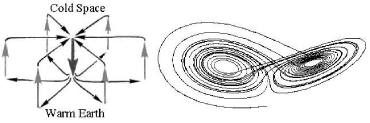
Figure 7: Bénard cells, showing a typical vortex of a rolling air, with a warm air rising in a ring and a cool air descending in the center (left). A simple model of a pair of Bénard cells given by the celebrated ‘Lorenz–butterfly’ (or, ‘Lorenz–mask’) strange attractor (right) [25].

The celebrated Lorenz ODEs read

$$\dot{x}=a(y-x),\qquad\dot{y}=bx-y-xz,\qquad\dot{z}=xy-cz,$$ (31)

where $x$, $y$ and $z$ are dynamical variables, constituting the 3D phase–space of the Lorenz system; and $a$, $b$ and $c$ are the parameters of the system. Originally, Lorenz used this model to describe the unpredictable behavior of the weather, where $x$ is the rate of convective overturning (convection is the process by which heat is transferred by a moving fluid), $y$ is the horizontal temperature overturning, and $z$ is the vertical temperature overturning; the parameters are: $a\equiv P-$proportional to the Prandtl number (ratio of the fluid viscosity of a substance to its thermal conductivity, usually set at $10$), $b\equiv R-$proportional to the Rayleigh number (difference in temperature between the top and bottom of the system, usually set at $28$), and $c\equiv K-$a number proportional to the physical proportions of the region under consideration (width to height ratio of the box which holds the system, usually set at $8/3$). The Lorenz system (31) has the properties:

1. Symmetry: $(x,y,z)\rightarrow(-x,-y,z)$ for all values of the parameters, and

2. The $z-$axis $(x=y=0)$ is invariant (i.e., all trajectories that start on it also end on it).

Nowadays it is well–known that the Lorenz model is a paradigm for low–dimensional chaos in dynamical systems in meteorology, hydrodynamics, laser physics, superconductivity, electronics, oil industry, chemical and biological kinetics, etc.

The 3D phase–portrait of the Lorenz system (7) shows the celebrated ‘Lorenz mask’, a special type of chaotic, strange, or, fractal attractor (see Figure 7). It depicts the famous ‘butterfly effect’, (i.e., sensitive dependence on initial conditions, that is, a tiny difference in initial conditions is amplified until two outcomes are totally different), so that the long term behavior becomes impossible to predict (e.g., long term weather forecasting). The Lorenz mask has the following characteristics: (i) trajectory does not intersect itself in three dimensions; (ii) trajectory is not periodic or transient; (iii) general form of the shape does not depend on initial conditions; and (iv) exact sequence of loops is very sensitive to the initial conditions.

References

- [1] R.A. Gatenby, P.K. Maini, Mathematical oncology: Cancer summed up. Nature, 421, 321, (2003)
- [2] T. Roose, S.J. Chapman, P.K. Maini, Mathematical Models of Avascular Tumor Growth. SIAM Rev. 49(2), 179–208, (2007).
- [3] V. Ivancevic, T. Ivancevic, Geometrical Dynamics of Complex Systems. Springer, Dordrecht, (2006)
- [4] V. Ivancevic, T. Ivancevic, Complex Dynamics: Advanced System Dynamics in Complex Variables. Springer, Dordrecht, (2007)
- [5] T. Ivancevic, L. Jain, J. Pattison, A. Hariz, Nonlinear Dynamics and Chaos Methods in Neurodynamics and Complex Data Analysis. Nonl. Dyn. (Springer) (to appear)
- [6] G. Guarini, E. Onofri, E. Menghetti, New horizons in medicine. The attractors. Recenti Prog. Med. (in Italian) 84(9), 618-623, (1993).
- [7] R. Sedivy, Fractal tumours: their real and virtual images. Wien Klin. Wochenschr. (in German) 108(17), 547-551, (1996).
- [8] R. Sedivy, C. Windischberger, Fractal analysis of a breast carcinoma–presentation of a modern morphometric method. Wien Klin. Wochenschr. (in German) 148(14), 335-337, (1998).
- [9] A.R.A. Anderson, M.A.J. Chaplain, Continuous and discrete mathematical models of tumor-induced angiogenesis. Bul. Math. Biol. 60, 857-000, (1998).
- [10] A.R.A. Anderson, M.A.J. Chaplain, E.L. Newman, R.J.C. Steele, A.M. Thompson, Mathematical modelling of tumour invasion and metastasis. J. Theor. Med. 2, 129 154, (2000).
- [11] A.R.A. Anderson, A hybrid mathematical model of solid tumour invasion: The importance of cell adhesion. Math. Med. Biol. 22, 163–186, (2005).
- [12] A.R.A. Anderson, A.M. Weaver, P.T.Cummings, V. Quaranta, Tumor Morphology and Phenotypic Evolution Driven by Selective Pressure from the Microenvironment. Cell 127, 905–915, (2006).
- [13] M.A.J. Chaplain, S.R. Mc Dougal, A.R.A. Anderson, Mathematical modelling of tumor-induced angiogenesis. Ann. Rev. Biomed. Eng. 8, 233-257, (2006).
- [14] H. Enderling, A.R.A. Anderson, M.A.J. Chaplain, Visualisation of the numerical solution of partial differential equation systems in three space dimensions and its importance for mathematical models in biology. Math. Biosci. Eng. 3(4), 571-582, (2006).
- [15] H. Enderling, M.A.J. Chaplain, A.R.A. Anderson, J.S. Vaidya, A mathematical model of breast cancer development, local treatment and recurrence. J. Th. Biol. 246, 245 259, (2007).
- [16] I. Ramis-Conde, M.A.J. Chaplain, A.R.A. Anderson, Mathematical modelling of cancer cell invasion of tissue. Math. Comp. Mod. 47, 533-545, (2008).
- [17] A. Gerish, M.A.J. Chaplain, Mathematical modelling of cancer cell invasion of tissue: Local and non-local models and the effect of adhesion. J. Th. Biol. 250, 684-704, (2008).
- [18] B.P. Marchant, J. Norbury, J.A. Sherratt, Travelling wave solutions to a haptotaxis-dominated model of malignant invasion. Nonlinearity, 14, 1653 1671, (2001)
- [19] E. Ott, C. Grebogi, J.A. Yorke, Controlling chaos. Phys. Rev. Lett., 64, 1196–1199, (1990).
- [20] V. Ivancevic, T. Ivancevic, High–Dimensional Chaotic and Attractor Systems. Springer, Berlin, (2006).
- [21] V. Ivancevic, T. Ivancevic, Complex Nonlinearity: Chaos, Phase Transitions, Topology Change and Path Integrals, Springer, Series: Understanding Complex Systems, Berlin, (in press).
- [22] E.N. Lorenz, Deterministic Nonperiodic Flow. J. Atmos. Sci., 20, 130–141, (1963).
- [23] C. Sparrow, The Lorenz Equations: Bifurcations, Chaos and Strange Attractors. Springer, New York, (1982).
- [24] V. Ivancevic, T. Ivancevic, Neuro-Fuzzy Associative Machinery for Comprehensive Brain and Cognition Modelling. Springer, Berlin, (2007)
- [25] V. Ivancevic, T. Ivancevic, Computational Mind: A Complex Dynamics Perspective. Springer, Berlin, (2007).
- [26] J.P. Sleeman, N. Cremers, New concepts in breast cancer metastasis: tumor initiating cells and the microenvironment. Clin. Exp. Metastasis. 24(8), 707–15, (2007).
- [27] I.P. Janecka, Cancer control through principles of systems science, complexity, and chaos theory: A model. Int. J. Med. Sci. 4(3), 164-173, (2007).
- [28] J.A. Downs, M.C. Nussenzweig, A. Nussenzweig, Chromatin dynamics and the preservation of genetic information. Nature, 447, 951-958, 21 June 2007.
- [29] I.M. Chu, L. Hengst, J.M. Slingerland, The Cdk inhibitor p27 in human cancer: prognostic potential and relevance to anticancer therapy. Nature Rev. Cancer, 8, 253-287, April 2008.
- [30] S. Cai, C.C. Lee, T. Kohwi-Shigematsu, SATB1 packages densely looped, transcriptionally active chromatin for coordinated expression of cytokine genes. Nature Genet. 38, 1278-1288, (2006).
- [31] H.-J. Han, J. Russo, Y. Kohwi, T. Kohwi-Shigematsu, SATB1 reprograms gene expression to promote breast tumor growth and metastasis. Nature, 452, 187 193, (2008).
- [32] Olive, P.L., Durand, R.E., Drug and radiation resistance in spheroids: cell contact and kinetics. Cancer Metastasis Rev. 13, 121, (1994).
- [33] Kozusko, F., Bourdeau, M., A unified model of sigmoid tumour growth based on cell proliferation and quiescence, Cell Prolif. 40(6), 824-834, (2007).
- [34] Castro, M.A.A., Klamt, F., Grieneisen, V.A., Grivicich, I., Moreira, J.C.F., Gompertzian growth pattern correlated with phenotypic organization of colon carcinoma, malignant glioma and non-small cell lung carcinoma cell lines. Cell Prolif. 36(2), 65-73, (2003).
- [35] Ingber, D.E., Fibronectin controls capillary endothelial cell growth by modulating cell shape. Proc. Natl. Acad. Sci. USA 87, 3579, (1990).
- [36] Boudreau, N., Jones, P.L., Extracellular matrix and integrin signaling: the shape of things to come. Biochem. J. 339, 481, (1999).