Branching ratios and CP asymmetries of $B\to K\eta^{(\prime)}$ decays in the pQCD approach

Abstract

We calculate the branching ratios and CP violating asymmetries of the four $B\to K\eta^{(\prime)}$ decays in the perturbative QCD (pQCD) factorization approach. Besides the full leading order contributions, the partial next-to-leading order (NLO) contributions from the QCD vertex corrections, the quark loops, and the chromo-magnetic penguins are also taken into account. The NLO pQCD predictions for the CP-averaged branching ratios are $Br(B^{+}\to K^{+}\eta)\approx 3.2\times 10^{-6}$, $Br(B^{\pm}\to K^{\pm}\eta^{\prime})\approx 51.0\times 10^{-6}$, $Br(B^{0}\to K^{0}\eta)\approx 2.1\times 10^{-6}$, and $Br(B^{0}\to K^{0}\eta^{\prime})\approx 50.3\times 10^{-6}$. The NLO contributions can provide a $70\%$ enhancement to the LO $Br(B\to K\eta^{\prime})$, but a $30\%$ reduction to the LO $Br(B\to K\eta)$, which play the key role in understanding the observed pattern of branching ratios. The NLO pQCD predictions for the CP-violating asymmetries, such as ${\cal A}_{CP}^{dir}(K^{0}_{S}\eta^{\prime})\sim 2.3\%$ and ${\cal A}_{CP}^{mix}(K^{0}_{S}\eta^{\prime})\sim 63\%$, agree very well with currently available data. This means that the deviation $\Delta S={\cal A}_{CP}^{mix}(K^{0}_{S}\eta^{\prime})-\sin{2\beta}$ in pQCD approach is also very small.

I Introduction

The $B\to K\eta^{(\prime)}$ decays are very interesting two-body charmless hadronic B meson decays. In 1997, CLEO collaboration firstly reported unexpectedly large branching ratios for $B\to K\eta^{\prime}$ decays cleo97 . Eleven years later, three of the four $B\to K\eta^{(\prime)}$ decays have been measured with high precision. The world averages as given by HFAG hfag are the following (in unit of $10^{-6}$)

$$Br(B^{\pm}\to K^{\pm}\eta) = 2.7\pm 0.3,$$

$$Br(B^{\pm}\to K^{\pm}\eta^{\prime}) = 70.2\pm 2.5,$$

$$Br(B^{0}\to K^{0}\eta) < 1.9,$$

$$Br(B^{0}\to K^{0}\eta^{\prime}) = 64.9\pm 3.1.$$ (1)

From above data one can see that: (a) the measured $Br(B\to K\eta^{\prime})$ are much larger than the early standard model (SM) expectations, i.e., the so-called $k\eta^{\prime}$-puzzle; and (b) the large disparity between the branching ratios for $B\to K\eta^{\prime}$ and $B\to K\eta$ decays: $Br(B\to K\eta^{\prime})\gg Br(B\to K\eta)$.

Besides the branching ratios, the CP violating asymmetries for $B^{\pm}\to K^{\pm}\eta^{(\prime)}$ and $B^{0}\to K^{0}\eta^{(\prime)}$ decays have been measured very recently hfag ; acpketap :

$${\cal A}_{CP}^{dir}(B^{\pm}\to K^{\pm}\eta) = -0.27\pm 0.09,$$

$${\cal A}_{CP}^{dir}(B^{\pm}\to K^{\pm}\eta^{\prime}) = 0.016\pm 0.019,$$ (2)

$${\cal A}_{CP}^{dir}(B^{0}\to K^{0}\eta^{\prime}) = 0.09\pm 0.06,$$

$${\cal A}_{CP}^{mix}(B^{0}\to K^{0}\eta^{\prime}) = 0.61\pm 0.07,$$ (3)

It may be noted that the average of the measured ${\cal A}_{CP}^{mix}(B^{0}\to K^{0}\eta^{\prime})$ is now more than $8\sigma$ away from zero, so that CP violation in this decay is well established; while ${\cal A}_{CP}^{dir}(B^{0}\to K^{0}\eta^{\prime})$ is not conflict with zero as expected in the SM. The data for ${\cal A}_{CP}^{dir}(B^{\pm}\to K^{\pm}\eta^{(\prime)})$ have less precision, but are consistent with general expectations.

The measurements of time-dependent CP asymmetries in $B^{0}$ meson decays, such as $B^{0}\to J/\Psi K^{0}$ via $b\to c\bar{c}s$ “tree” transition and $B^{0}\to K^{0}\eta^{\prime}$ via $b\to sq\bar{q}$ penguin transition, have provided crucial tests of the mechanism of CP violation in the SM. Within the SM the mixing induced CP violating asymmetry ${\cal A}_{CP}^{mix}(B^{0}\to K^{0}\eta^{\prime})=-\eta_{f}S_{f}$ should be comparable with $\sin 2\beta=0.685$ obtained from the tree dominated $B^{0}\to J/\Psi K^{0}$ decay, this point has been confirmed by the data in Eq. (3).

In the SM the decay $B\to K\eta^{(\prime)}$ is believed to proceed dominantly through gluonic penguin processeslipkin91 ; grossman and has been evaluated by employing various methods as97 ; chao97 ; ali98 ; du426 ; yy01 ; ahmady98 ; kagan ; xiao99 ; bn651 ; npb675 ; kou02 . Although great progress have been made during the past decade, but the predictions for $Br(B\to K\eta^{\prime})$ from both the QCD factorization (QCDF) approach bn651 ; bbns99 and the perturbative QCD (pQCD) approach kou02 ; li2003 in the Feldmann-Kroll-Stech (FKS) mixing scheme of $\eta-\eta^{\prime}$ system fks98 ; jhep0506 are smaller than the data.

For the pattern of branching ratios in Eq. (1), many possible solutions have been proposed. These include, for example,

• (a) Conventional $b\to sq\bar{q}$ with constructive (destructive) interference between the $u\bar{u},d\bar{d}$ and $s\bar{s}$ components of $\eta^{\prime}$ ($\eta$) lipkin91 ;

• (b) Large intrinsic charm content of $\eta^{\prime}$ through the chain $b\to sc\bar{c}\to s\eta^{\prime}$ chao97 or through $b\to sc\bar{c}\to sg^{*}g^{*}\to s(\eta,\eta^{\prime})$ due to the QCD anomaly ali98 ;

• (c) The spectator hard-scattering mechanism through the anomalous coupling of $gg\to\eta^{\prime}$ du426 ; yy01 ; ahmady98 ;

• (d) A significant flavor-singlet contribution yy01 ; bn651 ;

• (e) A strong penguin $b\to sg$ enhanced by new physics kagan ; xiao99 .

But the data of branching ratio in Eq. (1) are still not completely understood. For the CP violation of $B\to K\eta^{(\prime)}$ decays, the theoretical studies is still under way.

In Ref. kou02 , the authors calculated the branching ratios of $B\to K\eta^{(\prime)}$ decays by employing the pQCD approach at leading order. They considered the large corrections from $SU(3)$ flavor symmetry breaking as well as the possible gluonic component of $\eta^{\prime}$ meson, but their prediction for $Br(B^{0}\to K^{0}\eta^{\prime})$ ( $Br(B^{0}\to K^{0}\eta)$ ) is much smaller ( larger) than the measured value.

A sizable gluonic content in $\eta^{\prime}$ meson may provide a large enhancement to the decay rate of $B\to K\eta^{\prime}$. In Ref. li0609 , the authors examined the possible gluonic contribution to the $B\to\eta^{\prime}$ transition form factor and found that such contribution is constructive with those from quark-content of $\eta^{\prime}$, but numerically very small and can be neglected safely. This point has also been confirmed by the QCD sum-rule analysisbj0706

In the quark-flavor mixing scheme, the physical $\eta$ and $\eta^{\prime}$ meson are linear combinations of flavor state $\eta_{q}=(u\bar{u}+d\bar{d})/\sqrt{2}$ and $\eta_{s}=s\bar{s}$ with the ”mass” of $m_{qq}$ and $m_{ss}$ respectively. In Ref. acg07 , the effect of a large chiral scale $m_{0}^{q}=m_{qq}^{2}/(2m_{q})$ with $q=(u,d)$ for the meson $\eta_{q}$ has been evaluated although we do not know which mechanism is responsible to achieve a large value of $m_{qq}$. When one uses $m_{qq}=0.22$ GeV acg07 instead of its generally accepted value of $m_{qq}=0.11$ GeV, a larger $B\to K\eta_{q}$ decay amplitude can be obtained. Consequently, the LO pQCD predictions for $Br(B\to K\eta^{\prime})$ become consistent with the data.

In Ref. hsu07 , the authors examined the possible way to increase the value of $m_{qq}$. They found that few-percent violation of Okubo-Zweig-Iizuka (OZI) rule can enhance $m_{qq}$ few times, which then leads to the consistency of the LO predictions with the data for $B\to K\eta^{(\prime)}$ decays.

Besides the possible mechanisms mentioned above, we here consider a new and natural solution: the effects of the next-to-leading order (NLO) contributions in the pQCD approach. As shown in Ref. nlo05 , the NLO contributions to $B\to K\pi$ decays can play the key rule to explain the so-called $``K\pi"-$ puzzle. We expect here the NLO contributions could help us to resolve the $``K\eta^{\prime}"-$puzzle.

For the CP asymmetries of $B^{0}\to K^{0}\eta^{\prime}$, the deviation $\Delta S_{f}=-\eta_{f}S_{f}-\sin 2\beta$ has been estimated, for example, in the QCDF approach npb675 ; qcdf1 and the soft collinear effective theoryscet06 . The resultant bound is $|\Delta S_{f}|\lesssim 0.05$. Since the source of the CP violation in the pQCD approach is very different from those in the QCDF/SCET approach, we here try to calculate the CP asymmetries of $B\to K\eta^{(\prime)}$ decays by employing the pQCD approach at LO and NLO level, to check if we can accommodate the data of CP asymmetries.

In this paper we will calculate the next-to-leading order contributions to the branching ratios and CP violating asymmetries of the four $B\to K\eta^{(\prime)}$ decays. We firstly calculate the decay amplitudes of the $B\to K\eta^{(\prime)}$ decays by employing the pQCD factorization approach at the leading order (LO), as have been done in previous studies for other two-body charmless B meson decays kls01 ; luy01 ; xiao06 ; xiao07 . And then we evaluate the NLO contributions to these decays.

The NLO contributions considered here include: QCD vertex corrections, the quark-loops and the chromo-magnetic penguins. We wish that they are the major part of the full NLO contributions in pQCD approach nlo05 . Of course, remaining NLO contributions in pQCD approach, such as those from factorizable emission diagrams, hard-spectator and annihilation diagrams, should be calculated as soon as possible.

This paper is organized as follows. In Sec.II, we give a brief review about the pQCD factorization approach. In Sec. III, we calculate analytically the relevant Feynman diagrams and present the various decay amplitudes for the studied decay modes in leading-order. In Sec. IV, the NLO contributions from the vertex corrections, the quark loops and the chromo-magnetic penguin amplitudes are evaluated. We calculate and show the pQCD predictions for the branching ratios and CP violating asymmetries of $B\to K\eta^{(\prime)}$ decays in Sec. V. The summary and some discussions are included in the final section.

II Theoretical framework

II.1 Theoretical framework

In the pQCD approach, the decay amplitude is separated into soft ($\Phi_{M_{i}}$), hard ( $H(k_{i},t)$ ), and harder( $C(M_{W})$ ) dynamics characterized by different energy scales $(\Lambda_{QCD},t,m_{b},M_{W})$ li2003 . The decay amplitude ${\cal A}(B\to M_{2}M_{3})$ can be written conceptually as the convolution,

$${\cal A}(B\to M_{2}M_{3})\sim\int\!\!d^{4}k_{1}d^{4}k_{2}d^{4}k_{3}\ \mathrm{Tr}\left[C(t)\Phi_{B}(k_{1})\Phi_{M_{2}}(k_{2})\Phi_{M_{3}}(k_{3})H(k_{1},k_{2},k_{3},t)\right],$$ (4)

where $k_{i}$’s are momenta of light quarks included in each meson, and $\mathrm{Tr}$ denotes the trace over Dirac and color indices. $C(t)$ is the Wilson coefficient evaluated at scale $t$. In the above convolution, the Wilson coefficient $C(t)$ includes the harder dynamics at scale higher than $M_{B}$ and describes the evolution of local $4$-Fermi operators from $m_{W}$ ( the $W$ boson mass) down to $t\sim\mathcal{O}(\sqrt{\bar{\Lambda}M_{B}})$ scale, where $\bar{\Lambda}\equiv M_{B}-m_{b}$. The function $H(k_{1},k_{2},k_{3},t)$ describes the four quark operator and the spectator quark connected by a hard gluon whose $q^{2}$ is in the order of $\bar{\Lambda}M_{B}$, and includes the $\mathcal{O}(\sqrt{\bar{\Lambda}M_{B}})$ hard dynamics. Therefore, this hard kernel $H$ can be perturbatively calculated. The function $\Phi_{M_{i}}$ is the wave function which describes hadronization of the quark and anti-quark in the meson $M_{i}$. While the hard kernel $H$ depends on the processes considered, the wave function $\Phi_{M_{i}}$ is independent of the specific processes. Using the wave functions determined from other well measured processes, one can make quantitative predictions here.

Since the b quark inside the B meson is rather heavy, we consider the $B$ meson at rest for simplicity. It is then convenient to use light-cone coordinate $(p^{+},p^{-},{\bf p}_{\rm T})$ to describe the meson’s momenta: $p^{\pm}=\frac{1}{\sqrt{2}}(p^{0}\pm p^{3})$ and ${\bf p}_{\rm T}=(p^{1},p^{2})$ . Using the light-cone coordinates the $B$ meson momentum $P_{B}$ and the two final state meson’s momenta $P_{2}$ and $P_{3}$ (for $M_{2}$ and $M_{3}$ respectively) can be written as

$$P_{B}=\frac{M_{B}}{\sqrt{2}}(1,1,{\bf 0}_{\rm T}),\quad P_{2}=\frac{M_{B}}{\sqrt{2}}(1-r_{3}^{2},r^{2}_{2},{\bf 0}_{\rm T}),\quad P_{3}=\frac{M_{B}}{\sqrt{2}}(r_{3}^{2},1-r^{2}_{2},{\bf 0}_{\rm T}),$$ (5)

where $r_{i}=m_{i}/M_{B}$. $m_{2}$ and $m_{3}$ are the mass of the two final state mesons. For the case of $B\to PP$ decays, $r_{2}$ and $r_{3}$ are small and could be neglected safely.

Putting the anti-quark momenta in $B$, $M_{2}$ and $M_{3}$ meson as $k_{1}$, $k_{2}$, and $k_{3}$, respectively, we can choose

$$k_{1}=(x_{1}P_{1}^{+},0,{\bf k}_{\rm 1T}),\quad k_{2}=(x_{2}P_{2}^{+},0,{\bf k}_{\rm 2T}),\quad k_{3}=(0,x_{3}P_{3}^{-},{\bf k}_{\rm 3T}).$$ (6)

Then, the integration over $k_{1}^{-}$, $k_{2}^{-}$, and $k_{3}^{+}$ in eq.(4) will lead to

$${\cal A}(B\to PV) \sim \int\!\!dx_{1}dx_{2}dx_{3}b_{1}db_{1}b_{2}db_{2}b_{3}db_{3}$$ (7)

$$\cdot\mathrm{Tr}\left[C(t)\Phi_{B}(x_{1},b_{1})\Phi_{M_{2}}(x_{2},b_{2})\Phi_{M_{3}}(x_{3},b_{3})H(x_{i},b_{i},t)S_{t}(x_{i})\,e^{-S(t)}\right],\quad$$

where $b_{i}$ is the conjugate space coordinate of $k_{iT}$. The large logarithms ($\ln m_{W}/t$) coming from QCD radiative corrections to four quark operators are included in the Wilson coefficients $C(t)$. The large double logarithms ($\ln^{2}x_{i}$) on the longitudinal direction are summed by the threshold resummation, and they lead to $S_{t}(x_{i})$ which smears the end-point singularities on $x_{i}$. The last term, $e^{-S(t)}$, is the Sudakov form factor which suppresses the soft dynamics effectively li2003 .

II.2 Effective Hamiltonian and Wilson coefficients

For the studied $B\to K\eta^{(\prime)}$ decays, the weak effective Hamiltonian $H_{eff}$ for $b\to s$ transition can be written as buras96

$${\cal H}_{eff}=\frac{G_{F}}{\sqrt{2}}\,\sum_{q=u,c}V_{qb}V_{qs}^{*}\left\{\left[C_{1}(\mu)O_{1}^{q}(\mu)+C_{2}(\mu)O_{2}^{q}(\mu)\right]+\sum_{i=3}^{10}C_{i}(\mu)\;O_{i}(\mu)\right\}\;.$$ (8)

where $G_{F}=1.16639\times 10^{-5}GeV^{-2}$ is the Fermi constant, and $V_{ij}$ is the CKM matrix element, $C_{i}(\mu)$ are the Wilson coefficients evaluated at the renormalization scale $\mu$ and $O_{i}(\mu)$ are the four-fermion operators. For the case of $b\to d$ transition, simply makes a replacement of $s$ by $d$ in Eq. (8) and in the expressions of $O_{i}(\mu)$ operators, which can be found easily for example in Refs.xiao06 ; xiao07 ; buras96 .

In PQCD approach, the energy scale $``t"$ is chosen as the largest energy scale in the hard kernel $H(x_{i},b_{i},t)$ of a given Feynman diagram, in order to suppress the higher order corrections and improve the reliability of the perturbative calculation. Here, the scale $``t"$ may be larger or smaller than the $m_{b}$ scale. In the range of $t<m_{b}$ or $t\geq m_{b}$, the number of active quarks is $N_{f}=4$ or $N_{f}=5$, respectively. For the Wilson coefficients $C_{i}(\mu)$ and their renormalization group (RG) running, they are known at NLO level currently buras96 . The explicit expressions of the LO and NLO $C_{i}(m_{W})$ can be found easily, for example, in Refs. luy01 ; buras96 .

When the pQCD approach at leading-order are employed, the leading order Wilson coefficients $C_{i}(m_{W})$, the leading order RG evolution matrix $U(t,m)^{(0)}$ from the high scale $m$ down to $t<m$ ( for details see Eq. (3.94) in Ref. buras96 ), and the leading order $\alpha_{s}(t)$ are used:

$$\alpha_{s}(t)=\frac{4\pi}{\beta_{0}\ln\left[t^{2}/\Lambda_{QCD}^{2}\right]},$$ (9)

where $\beta_{0}=(33-2N_{f})/3$, $\Lambda_{QCD}^{(5)}=0.225GeV$ and $\Lambda_{QCD}^{(4)}=0.287$ GeV.

When the NLO contributions are taken into account, however, the NLO Wilson coefficients $C_{i}(m_{W})$, the NLO RG evolution matrix $U(t,m,\alpha)$ ( for details see Eq. (7.22) in Ref. buras96 ) and the $\alpha_{s}(t)$ at two-loop level are used:

$$\alpha_{s}(t)=\frac{4\pi}{\beta_{0}\ln\left[t^{2}/\Lambda_{QCD}^{2}\right]}\cdot\left\{1-\frac{\beta_{1}}{\beta_{0}^{2}}\cdot\frac{\ln\left[\ln\left[t^{2}/\Lambda_{QCD}^{2}\right]\right]}{\ln\left[t^{2}/\Lambda_{QCD}^{2}\right]}\right\},$$ (10)

where $\beta_{0}=(33-2N_{f})/3$, $\beta_{1}=(306-38N_{f})/3$, $\Lambda_{QCD}^{(5)}=0.225$ GeV and $\Lambda_{QCD}^{(4)}=0.326$ GeV.

From the general knowledge, the hard scale $t$ must be much larger than $\Lambda_{QCD}\approx 0.2$ GeV in order to guarantee the reliability of perturbative calculations. In previous calculations based on the pQCD approach $\mu_{0}=0.5$ GeV is chosen as the lower cut-off of the scale $t$. In our opinion, it is indeed too low, because it may be conceptually incorrect to evaluate the Wilson coefficients at scales down to $0.5$ GeV  beneke07 . The explicit numerical checks as done in Ref. xiao08a also show that (a) the Wilson coefficient $C_{1}(0.5)$ is close to $-1$ and clearly too large in size! (b) the values of the Wilson coefficients $C_{3,4,5,6}(\mu)$ at $\mu=0.5$ GeV are about four to seven times larger than those at $\mu=1.0$ GeV; and (c) the $\mu_{0}-$dependence of all Wilson coefficients become relatively weak for $\mu_{0}\geq 1.0$ GeV. We therefore believe that it is reasonable to choose $\mu_{0}=1.0$ GeV as the lower cut-off of the hard scale $t$, which is also close to the hard-collinear scale $\sqrt{\bar{\Lambda}m_{B}}\sim 1.3$ GeV in SCET. In the numerical integrations we will fix the values $C_{i}(t)$ at $C_{i}(1.0)$ whenever the scale $t$ runs below the scale $\mu_{0}=1.0$ GeV xiao08a ; xiao08b .

II.3 Wave functions

Since the b-quark is much heavier than the up or down quark, the $B$ meson is treated as a very good heavy-light system. Although there are in general two Lorentz structures in the B meson distribution amplitudes, they obey to the following normalization conditions

$$\int\frac{d^{4}k_{1}}{(2\pi)^{4}}\phi_{B}({\bf k_{1}})=\frac{f_{B}}{2\sqrt{2N_{c}}},~{}~{}~{}\int\frac{d^{4}k_{1}}{(2\pi)^{4}}\bar{\phi}_{B}({\bf k_{1}})=0.$$ (11)

However, it can be argued that the contribution of $\bar{\phi}_{B}$ is numerically small  luyang , thus its contribution can be numerically neglected. In this approximation, we only consider the contribution of Lorentz structure

$$\Phi_{B}=\frac{1}{\sqrt{2N_{c}}}(P/_{B}+m_{B})\gamma_{5}\phi_{B}({\bf k_{1}}),$$ (12)

with

$$\phi_{B}(x,b) = N_{B}x^{2}(1-x)^{2}\mathrm{exp}\left[-\frac{M_{B}^{2}\ x^{2}}{2\omega_{b}^{2}}-\frac{1}{2}(\omega_{b}b)^{2}\right],$$ (13)

where $\omega_{b}$ is a free parameter and we take $\omega_{b}=0.4\pm 0.04$ GeV in numerical calculations, and $N_{B}=101.445$ is the normalization factor for $\omega_{b}=0.4$.

The Kaon mesons are treated as a light-light system. The wave function of $K$ meson is defined as ball98

$$\Phi_{K}(P,x,\zeta)\equiv\frac{1}{\sqrt{2N_{C}}}\gamma_{5}\left[P/\phi_{K}^{A}(x)+m_{0}^{K}\phi_{K}^{P}(x)+\zeta m_{0}^{K}(v/n/-v\cdot n)\phi_{K}^{T}(x)\right],$$ (14)

where $P$ and $x$ are the momentum and the momentum fraction of $K$, respectively. The parameter $\zeta$ is either $+1$ or $-1$ depending on the assignment of the momentum fraction $x$.

For $\eta^{(\prime)}$ meson, the wave function for $\eta_{q}$ components of $\eta^{\prime}$ meson are given as

$$\Phi_{\eta_{q}}(P,x,\zeta)\equiv\frac{1}{\sqrt{2N_{C}}}\gamma_{5}\left[P/\phi_{\eta_{q}}^{A}(x)+m_{0}^{q}\phi_{\eta_{q}}^{P}(x)+\zeta m_{0}^{q}(v/n/-v\cdot n)\phi_{\eta_{q}}^{T}(x)\right],$$ (15)

where $P$ and $x$ are the momentum and the momentum fraction of $\eta_{q}$, respectively. We assumed here that the wave function of $\eta_{q}$ is same as the $\pi$ wave function. The parameter $\zeta$ is either $+1$ or $-1$ depending on the assignment of the momentum fraction $x$. The $\eta_{s}=s\bar{s}$ component of the wave function can be defined in the same way.

The expressions of the relevant distribution amplitudes (DA’s) of K meson are the following ball98 :

$$\phi_{K}^{A}(x) = \frac{f_{K}}{2\sqrt{2N_{c}}}6x(1-x)\left[1+a_{1}^{K}C^{3/2}_{1}(t)+a^{K}_{2}C^{3/2}_{2}(t)+a^{K}_{4}C^{3/2}_{4}(t)\right],$$ (16)

$$\phi_{K}^{P}(x) = \frac{f_{K}}{2\sqrt{2N_{c}}}\left\{1+(30\eta_{3}-\frac{5}{2}\rho^{2}_{K})C^{1/2}_{2}(t)-3\left[\eta_{3}\omega_{3}+\frac{9}{20}\rho^{2}_{K}(1+6a^{K}_{2})\right]C^{1/2}_{4}(t)\right\},\ \$$ (17)

$$\phi_{K}^{T}(x) = -\frac{f_{K}}{2\sqrt{2N_{c}}}t\left[1+6(5\eta_{3}-\frac{1}{2}\eta_{3}\omega_{3}-\frac{7}{20}\rho^{2}_{K}-\frac{3}{5}\rho^{2}_{K}a_{2}^{K})(1-10x+10x^{2})\right],\quad\quad$$ (18)

with the mass ratio $\rho_{K}=m_{K}/m_{0K}$. The Gegenbauer moments can be given as ball98 :

$$a^{K}_{1}=0.2,\quad a^{K}_{2}=0.25,\quad a^{K}_{4}=-0.015.$$ (19)

The values of other parameters are $\eta_{3}=0.015$ and $\omega=-3.0$. At last the Gegenbauer polynomials $C^{\nu}_{n}(t)$ are given as:

$$C^{1/2}_{2}(t) = \frac{1}{2}(3t^{2}-1),\qquad C^{1/2}_{4}(t)=\frac{1}{8}(3-30t^{2}+35t^{4}),$$

$$C^{3/2}_{1}(t) = 3t,\qquad C^{3/2}_{2}(t)=\frac{3}{2}(5t^{2}-1),$$

$$C^{3/2}_{4}(t) = \frac{15}{8}(1-14t^{2}+21t^{4}),$$ (20)

with $t=2x-1$.

In the quark-flavor mixing scheme, the physical states $\eta$ and $\eta^{\prime}$ are related to the flavor states $\eta_{q}=(u\bar{u}+d\bar{d})/\sqrt{2}$ and $\eta_{s}=s\bar{s}$ through a single mixing angle $\phi$,

$$\left(\begin{array}[]{c}\eta\\ \eta^{\prime}\end{array}\right)=\left(\begin{array}[]{cc}\cos{\phi}&-\sin{\phi}\\ \sin{\phi}&\cos{\phi}\\ \end{array}\right)\left(\begin{array}[]{c}\eta_{q}\\ \eta_{s}\end{array}\right)=\left(\begin{array}[]{c}F_{1}(\phi)(u\bar{u}+d\bar{d})+F_{2}(\phi)\;s\bar{s}\\ F_{1}^{\prime}(\phi)(u\bar{u}+d\bar{d})+F_{2}^{\prime}(\phi)\;s\bar{s}\\ \end{array}\right)$$ (29)

with

$$F_{1}(\phi) = \frac{\cos\phi}{\sqrt{2}},\quad F_{2}(\phi)=-\sin\phi,$$

$$F_{1}^{\prime}(\phi) = \frac{\sin\phi}{\sqrt{2}},\quad F_{2}^{\prime}(\phi)=\cos\phi.$$ (30)

The relation between the decay constants $(f_{\eta}^{q},f_{\eta}^{s},f_{\eta^{\prime}}^{q},f_{\eta^{\prime}}^{s})$ and $(f_{q},f_{s},)$ can be written as

$$\left(\begin{array}[]{cc}f^{q}_{\eta}&f^{s}_{\eta}\\ f^{q}_{\eta^{\prime}}&f^{s}_{\eta^{\prime}}\end{array}\right)=\left(\begin{array}[]{cc}\cos{\phi}&-\sin{\phi}\\ \sin{\phi}&\cos{\phi}\\ \end{array}\right)\left(\begin{array}[]{cc}f_{q}&0\\ 0&f_{s}\end{array}\right),$$ (37)

The chiral enhancement $m_{0}^{q}$ and $m_{0}^{s}$ associated with the two-parton twist-3 $\eta_{q}$ and $\eta_{s}$ meson distribution amplitudes have been defined as nlo05

$$m^{q}_{0} = \frac{m^{2}_{qq}}{2m_{q}}=\frac{1}{2m_{q}}[m^{2}_{\eta}\cos^{2}\phi+m^{2}_{\eta^{\prime}}\sin^{2}\phi-\frac{\sqrt{2}f_{s}}{f_{q}}(m^{2}_{\eta^{\prime}}-m^{2}_{\eta})\cos\phi\sin\phi],$$ (38)

$$m^{s}_{0} = \frac{m^{2}_{ss}}{2m_{s}}=\frac{1}{2m_{s}}[m^{2}_{\eta^{\prime}}\cos^{2}\phi+m^{2}_{\eta}\sin^{2}\phi-\frac{\sqrt{2}f_{q}}{f_{s}}(m^{2}_{\eta^{\prime}}-m^{2}_{\eta})\cos\phi\sin\phi],$$ (39)

by assuming the exact isospin symmetry $m_{q}=m_{u}=m_{d}$. The three input parameters $f_{q},f_{s}$ and $\phi$ have been extracted from the data of the relevant exclusive processes fks98 :

$$f_{q}=(1.07\pm 0.02)f_{\pi},\quad f_{s}=(1.34\pm 0.06)f_{\pi},\quad\phi=39.3^{\circ}\pm 1.0^{\circ},$$ (40)

The distribution amplitudes $\phi_{\eta_{q}}^{A,P,T}$ represent the axial vector, pseudoscalar and tensor component of the wave function respectively ball98 . They are given as:

$$\phi_{\eta_{q}}^{A}(x) = \frac{f_{q}}{2\sqrt{2N_{c}}}6x(1-x)\left[1+a^{\eta_{q}}_{1}C^{3/2}_{1}(2x-1)+a^{\eta_{q}}_{2}C^{3/2}_{2}(2x-1)\right.$$ (41)

$$\left.+a^{\eta_{q}}_{4}C^{3/2}_{4}(2x-1)\right],$$

$$\phi_{\eta_{q}}^{P}(x) = \frac{f_{q}}{2\sqrt{2N_{c}}}\left[1+(30\eta_{3}-\frac{5}{2}\rho^{2}_{\eta_{q}})C^{1/2}_{2}(2x-1)\right.$$ (42)

$$\left.-3\left\{\eta_{3}\omega_{3}+\frac{9}{20}\rho^{2}_{\eta_{q}}(1+6a^{\eta_{q}}_{2})\right\}C^{1/2}_{4}(2x-1)\right],$$

$$\phi_{\eta_{q}}^{T}(x) = \frac{f_{q}}{2\sqrt{2N_{c}}}(1-2x)\left[1+6\left(5\eta_{3}-\frac{1}{2}\eta_{3}\omega_{3}-\frac{7}{20}\rho^{2}_{\eta_{q}}-\frac{3}{5}\rho^{2}_{\eta_{q}}a_{2}^{\eta_{q}}\right)\right.$$ (43)

$$\left.\cdot\left(1-10x+10x^{2}\right)\right],\quad\quad$$

where $\rho_{\eta_{q}}=2m_{q}/m_{qq}$,$a^{\eta_{q}}_{1}=a_{1}^{\pi}=0$, $a^{\eta_{q}}_{2}=a_{2}^{\pi}=0.44\pm 0.22$, $a^{\eta_{q}}_{4}=a_{4}^{\pi}=0.25$, and the Gegenbauer polynomials $C^{\nu}_{n}(t)$ have been given in Eq. (20). As to the wave function and the corresponding DA’s of the $s\bar{s}$ components, we also use the same form as $q\bar{q}$ but with some parameters changed: $\rho_{\eta_{s}}=2m_{s}/m_{ss}$, $a^{\eta_{s}}_{i}=a^{\eta_{q}}_{i}$ for $i=1,2,4$.

The transverse momentum $k_{T}$ is usually converted to the $b$ parameter by Fourier transformation. The initial conditions of leading twist $\phi_{i}(x)$, $i=B,K,\eta,\eta^{\prime}$, are of non-perturbative origin, satisfying the normalization

$$\int_{0}^{1}\phi_{i}(x,b=0)dx=\frac{1}{2\sqrt{6}}{f_{i}}\;,$$ (44)

with $f_{i}$ the meson decay constant.

III Decay amplitudes at leading order

Figure 1: Feynman diagrams which may contribute to the $B\to K\eta^{(\prime)}$ decays at leading order.

In the pQCD approach, the Feynman diagrams as shown in Fig. 1 may contribute to $B\to K\eta^{(\prime)}$ decays at leading order. As mentioned previously, $B^{0}\to K^{0}\eta^{(\prime)}$ decays have been studied in Ref. kou02 by employing the LO pQCD approach. In this section, we firstly calculate the LO decay amplitudes for four $B\to K\eta^{(\prime)}$ decays, but in a rather different way to treat the Feynman diagrams from that in Ref. kou02 .

At the leading order in pQCD approach, there are three type diagrams contributing to the $B\to K\eta^{(\prime)}$ decays, the factorizable emission diagrams, the hard-spectator diagrams and the annihilation diagrams, as illustrated in Fig.1. From the factorizable emission diagrams, the corresponding form factors can be extracted by perturbative calculation. First, we consider the $B\to K\eta$ decay modes, and then extend the calculation to $B\to K\eta^{\prime}$ decays.

For the usual factorizable emission diagrams 1(a) and 1(b) with the $B\to K$ transition, i.e., it is the K meson pick up the spectator quark, the operators $O_{1}$, $O_{2}$, $O_{3,4}$ and $O_{9,10}$ are $(V-A)(V-A)$ currents, the sum of the individual amplitudes is given as

$$F_{eK} = \frac{8}{\sqrt{2}}\pi G_{F}C_{F}m_{B}^{4}\;\int_{0}^{1}dx_{1}dx_{2}\,\int_{0}^{\infty}b_{1}db_{1}b_{2}db_{2}\,\phi_{B}(x_{1},b_{1})$$ (45)

$$\times\left\{\left[(1+x_{2})\phi_{K}^{A}(\bar{x}_{2})+(1-2x_{2})r_{K}(\phi_{K}^{P}(\bar{x}_{2})-\phi_{K}^{T}(\bar{x}_{2}))\right]\cdot E_{e}(t_{a})h_{e}(x_{1},x_{2},b_{1},b_{2})\right.$$

$$\left.+2r_{K}\phi_{K}^{P}(\bar{x}_{2})\cdot E_{e}(t_{a}^{\prime})h_{e}(x_{2},x_{1},b_{2},b_{1})\right\},$$

where $r_{K}=m_{0}^{K}/m_{B}$ with $m_{0}^{K}$ is the chiral scale; $C_{F}=4/3$ is a color factor, and $\bar{x}_{2}=1-x_{2}$. The evolution function $E_{e}(t)$ and hard function $h_{e}$ are displayed in Appendix A. In the above equation, we do not include the Wilson coefficients of the corresponding operators, which are process dependent. They will be shown later in the expressions of total decay amplitude.

Also for diagrams 1(a) and 1(b), the operators $O_{5,6}$ and $O_{7,8}$ have a structure of $(V-A)(V+A)$ currents. In some decay channels, some of these operators contribute to the decay amplitude in a factorizable way. Since only the axial-vector part of $(V+A)$ current contribute to the pseudo-scaler meson production, $\langle K|V-A|B\rangle\langle\eta^{(\prime)}|V+A|0\rangle=-\langle K|V-A|B\rangle\langle\eta^{(\prime)}|V-A|0\rangle,$ that is

$$F_{eK}^{P1}=-F_{eK}\;.$$ (46)

In some other cases, we need to do Fierz transformation for those operators to get right color structure for factorization to work. In this case, we get $(S-P)(S+P)$ operators from $(V-A)(V+A)$ ones. For these $(S-P)(S+P)$ operators, the corresponding decay amplitude is

$$F_{eK}^{P2} = \frac{16}{\sqrt{2}}\pi G_{F}C_{F}m_{B}^{4}\int_{0}^{1}dx_{1}dx_{2}\,\int_{0}^{\infty}b_{1}db_{1}b_{2}db_{2}\,\phi_{B}(x_{1})$$ (47)

$$\times\left\{r_{\eta}\left[\phi_{K}^{A}(\bar{x}_{2})+r_{K}((2+x_{2})\phi_{K}^{P}(\bar{x}_{2})+x_{2}\phi_{K}^{T}(\bar{x}_{2}))\right]\cdot E_{e}(t_{a})h_{e}(x_{1},x_{2},b_{1},b_{2})\right.$$

$$\left.\ +2r_{K}r_{\eta}\phi_{K}^{P}(\bar{x}_{2})\cdot E_{e}(t_{a}^{\prime})h_{e}(x_{2},x_{1},b_{2},b_{1})\right\}\;.$$

where $r_{\eta}=m_{0}^{q}/m_{B}$, and $m_{0}^{q}=m_{0}^{\eta_{q}}$ is the chiral scale defined in Eq. (38).

For the non-factorizable diagrams 1(c) and 1(d), all three meson wave functions are involved. The integration of $b_{2}$ can be performed using $\delta$ function $\delta(b_{3}-b_{2})$, leaving only integration of $b_{1}$ and $b_{3}$. For the $(V-A)(V-A)$ operators, the result is

$$M_{eK} = \frac{16}{\sqrt{3}}\pi G_{F}C_{F}m_{B}^{4}\;\int_{0}^{1}dx_{1}dx_{2}\,dx_{3}\,\int_{0}^{\infty}b_{1}db_{1}b_{3}db_{3}\,\phi_{B}(x_{1},b_{1})\phi_{\eta}^{A}(\bar{x}_{3})$$ (48)

$$\times\left\{\left[-r_{K}x_{2}\left(\phi_{K}^{P}(\bar{x}_{2})+\phi_{K}^{T}(\bar{x}_{2})\right)+(1-x_{3})\phi_{K}^{A}(\bar{x}_{2})\right]\right.$$

$$\left.\ \ \ \cdot E_{e}^{\prime}(t_{b})h_{n}(x_{1},x_{2},1-x_{3},b_{1},b_{3})\right.$$

$$\left.+\left[-(x_{2}+x_{3})\phi_{K}^{A}(\bar{x}_{2})+r_{K}x_{2}\left(\phi_{K}^{P}(\bar{x}_{2})-\phi_{K}^{T}(\bar{x}_{2})\right)\right]\right.$$

$$\left.\ \ \ \cdot E_{e}^{\prime}(t_{b}^{\prime})h_{n}(x_{1},x_{2},x_{3},b_{1},b_{3})\right\},$$

where $\phi_{\eta}$ denotes $\phi_{\eta_{q}}$ or $\phi_{\eta_{s}}$.

There are two kinds of contributions from $(V-A)(V+A)$ operators: $M_{eK}^{P1}$ and $M_{eK}^{P2}$, corresponding to the $(V-A)(V+A)$ and $(S-P)(S+P)$ type operators respectively:

$$M_{eK}^{P1} = \frac{16}{\sqrt{3}}\pi G_{F}C_{F}m_{B}^{4}\;\int_{0}^{1}dx_{1}dx_{2}\,dx_{3}\,\int_{0}^{\infty}b_{1}db_{1}b_{3}db_{3}\,\phi_{B}(x_{1},b_{1})$$ (49)

$$\cdot\left\{\left[(1-x_{3})\phi_{K}^{A}(\bar{x}_{2})\left(\phi_{\eta}^{P}(\bar{x}_{3})-\phi_{\eta}^{T}(\bar{x}_{3})\right)\right.\right.$$

$$\left.\left.+r_{K}(1-x_{3})\left(\phi_{K}^{P}(\bar{x}_{2})+\phi_{K}^{T}(\bar{x}_{2})\right)\left(\phi_{\eta}^{P}(\bar{x}_{3})-\phi_{\eta}^{T}(\bar{x}_{3})\right)\right.\right.$$

$$\left.\left.+r_{K}x_{2}\left(\phi_{K}^{P}(\bar{x}_{2})-\phi_{K}^{T}(\bar{x}_{2})\right)\left(\phi_{\eta}^{P}(\bar{x}_{3})+\phi_{\eta}^{T}(\bar{x}_{3})\right)\right]\right.$$

$$\left.\ \ \cdot E_{e}^{\prime}(t_{b})h_{n}(x_{1},x_{2},1-x_{3},b_{1},b_{3})\right.$$

$$\left.-\left[\;x_{3}\phi_{K}^{A}(\bar{x}_{2})\left(\phi_{\eta}^{P}(\bar{x}_{3})+\phi_{\eta}^{T}(\bar{x}_{3})\right)\right.\right.$$

$$\left.\left.+r_{2}x_{3}\left(\phi_{K}^{P}(\bar{x}_{2})+\phi_{K}^{T}(\bar{x}_{2})\right)\left(\phi_{\eta}^{P}(\bar{x}_{3})+\phi_{\eta}^{T}(\bar{x}_{3})\right)\right.\right.$$

$$\left.\left.+r_{2}x_{2}\left(\phi_{K}^{P}(\bar{x}_{2})-\phi_{K}^{T}(\bar{x}_{2})\right)\left(\phi_{\eta}^{P}(\bar{x}_{3})-\phi_{\eta}^{T}(\bar{x}_{3})\right)\;\right]\right.$$

$$\left.\ \ \cdot E_{e}^{\prime}(t_{b}^{\prime})h_{n}(x_{1},x_{2},x_{3},b_{1},b_{3})\right\},$$

$$M_{eK}^{P2} = \frac{16}{\sqrt{3}}\pi G_{F}C_{F}m_{B}^{4}\int_{0}^{1}dx_{1}dx_{2}\,dx_{3}\,\int_{0}^{\infty}b_{1}db_{1}b_{3}db_{3}\,\phi_{B}(x_{1},b_{1})\phi_{\eta}^{A}(\bar{x}_{3})$$ (50)

$$\cdot\left\{\left[-(1+x_{2}-x_{3})\phi_{K}^{A}(\bar{x}_{2})+x_{2}r_{K}\left(\phi_{K}^{P}(\bar{x}_{2})-\phi_{K}^{T}(\bar{x}_{2})\right)\right]\right.$$

$$\left.\ \ \cdot E_{e}^{\prime}(t_{b})h_{n}(x_{1},x_{2},1-x_{3},b_{1},b_{3})\right.$$

$$\left.+\left[x_{3}\phi_{K}^{A}(\bar{x}_{2})-x_{2}r_{K}\left(\phi_{K}^{P}(\bar{x}_{2})+\phi_{K}^{T}(\bar{x}_{2})\right)\right]\cdot E_{e}^{\prime}(t_{b}^{\prime})h_{n}(x_{1},x_{2},x_{3},b_{1},b_{3})\right\}.$$

For the non-factorizable annihilation diagrams 1(e) and 1(f), again all three wave functions are involved. Here we have two kinds of contributions: $M_{aK}^{P2}=0$, $M_{aK}$ and $M_{aK}^{P1}$ describe the contributions from the $(V-A)(V-A)$ and $(V-A)(V+A)$ type operators, respectively,

$$M_{aK} = \frac{16}{\sqrt{3}}\pi G_{F}C_{F}m_{B}^{4}\;\int_{0}^{1}dx_{1}dx_{2}\,dx_{3}\,\int_{0}^{\infty}b_{1}db_{1}b_{3}db_{3}\,\phi_{B}(x_{1},b_{1})$$ (51)

$$\cdot\left\{\left[(1-x_{2})\phi_{K}^{A}(\bar{x}_{2})\phi_{\eta}^{A}(\bar{x}_{3})+r_{K}r_{\eta}(1-x_{2})\left(\phi_{K}^{P}(\bar{x}_{2})+\phi_{K}^{T}(\bar{x}_{2})\right)\left(\phi_{\eta}^{P}(\bar{x}_{3})-\phi_{\eta}^{T}(\bar{x}_{3})\right)\right.\right.$$

$$\left.\left.+r_{K}r_{\eta}x_{3}\left(\phi_{K}^{P}(\bar{x}_{2})-\phi_{K}^{T}(\bar{x}_{2})\right)\left(\phi_{\eta}^{P}(\bar{x}_{3})+\phi_{\eta}^{T}(\bar{x}_{3})\right)\right]\cdot E_{a}^{\prime}(t_{c})h_{na}(x_{1},x_{2},x_{3},b_{1},b_{3})\right.$$

$$\left.-\left[x_{3}\phi_{K}^{A}(\bar{x}_{2})\phi_{\eta}^{A}(\bar{x}_{3})+4r_{K}r_{\eta}\phi_{K}^{P}(\bar{x}_{2})\phi_{\eta}^{P}(\bar{x}_{3})-r_{K}r_{\eta}(1-x_{3})\left(\phi_{K}^{P}(\bar{x}_{2})+\phi_{K}^{T}(\bar{x}_{2})\right)\right.\right.$$

$$\cdot\left.\left.\left(\phi_{\eta}^{P}(\bar{x}_{3})-\phi_{\eta}^{T}(\bar{x}_{3})\right)-r_{K}r_{\eta}x_{2}\left(\phi_{K}^{P}(\bar{x}_{2})-\phi_{K}^{T}(\bar{x}_{2})\right)\left(\phi_{\eta}^{P}(\bar{x}_{3})+\phi_{\eta}^{T}(\bar{x}_{3})\right)\right]\right.$$

$$\times\left.\ \ \cdot E_{a}^{\prime}(t_{c}^{\prime})h_{na}(x_{1},x_{2},x_{3},b_{1},b_{3})\right\}\;,$$

$$M_{aK}^{P1} = \frac{16}{\sqrt{3}}\pi G_{F}C_{F}m_{B}^{4}\int_{0}^{1}dx_{1}dx_{2}\,dx_{3}\,\int_{0}^{\infty}b_{1}db_{1}b_{3}db_{3}\,\phi_{B}(x_{1},b_{1})$$ (52)

$$\times\left\{\left[-(1-x_{2})r_{K}\phi_{\eta}^{A}(\bar{x}_{3})\left(\phi_{K}^{P}(\bar{x}_{2})+\phi_{K}^{T}(\bar{x}_{2})\right)+r_{\eta}x_{3}\phi_{K}^{A}(\bar{x}_{2})\left(\phi_{\eta}^{P}(\bar{x}_{3})-\phi_{\eta}^{T}(\bar{x}_{3})\right)\right]\right.$$

$$\left.\times E_{a}^{\prime}(t_{c})h_{na}(x_{1},x_{2},x_{3},b_{1},b_{3})-\left[(x_{2}+1)r_{K}\phi_{\eta}^{A}(\bar{x}_{3})\left(\phi_{K}^{P}(\bar{x}_{2})+\phi_{K}^{T}(\bar{x}_{2})\right)\right.\right.$$

$$\left.\left.+r_{\eta}(x_{3}-2)\phi_{K}^{A}(\bar{x}_{2})\left(\phi_{\eta}^{P}(\bar{x}_{3})-\phi_{\eta}^{T}(\bar{x}_{3})\right)\right]E_{a}^{\prime}(t_{c}^{\prime})h_{na}(x_{1},x_{2},x_{3},b_{1},b_{3})\right\}\;.$$

The factorizable annihilation diagrams 1(g) and 1(h) involve only $K$ and $\eta^{(\prime)}$ wave functions. There are also three kinds of decay amplitudes for these two diagrams. $F_{aK}$, $F_{aK}^{P1}$ and $F_{aK}^{P2}$:

$$F_{aK} = F_{aK}^{P1}=\frac{8}{\sqrt{2}}\pi G_{F}C_{F}m_{B}^{4}\;\int_{0}^{1}dx_{2}\,dx_{3}\,\int_{0}^{\infty}b_{2}db_{2}b_{3}db_{3}\,\left\{-\left[(1-x_{2})\phi_{K}^{A}(\bar{x}_{2})\phi_{\eta}^{A}(\bar{x}_{3})\right.\right.$$ (53)

$$\left.\left.+4r_{\eta}r_{K}\phi_{K}^{P}(\bar{x}_{2})\phi_{\eta}^{P}(\bar{x}_{3})-2r_{K}r_{\eta}x_{2}\phi_{\eta}^{P}(\bar{x}_{3})\left(\phi_{K}^{P}(\bar{x}_{2})+\phi_{K}^{T}(\bar{x}_{2})\right)\right]\right.$$

$$\left.\ \ \cdot E_{a}(t_{d})h_{a}(x_{3},1-x_{2},b_{3},b_{2})\right.$$

$$\left.+\left[x_{3}\phi_{K}^{A}(\bar{x}_{2})\phi_{\eta}^{A}(\bar{x}_{3})+2r_{\eta}r_{K}\phi_{K}^{P}(\bar{x}_{2})\left(\phi_{\eta}^{P}(\bar{x}_{3})+\phi_{\eta}^{T}(\bar{x}_{3})\right)\right.\right.$$

$$\left.\left.+2r_{\eta}r_{K}x_{3}\phi_{K}^{P}(\bar{x}_{2})\left(\phi_{\eta}^{P}(\bar{x}_{3})-\phi_{\eta}^{T}(\bar{x}_{3})\right)\right]\cdot E_{a}(t_{d}^{\prime})h_{a}(1-x_{2},x_{3},b_{2},b_{3})\right\}\;,$$

$$F_{aK}^{P2} = \frac{16}{\sqrt{2}}\pi G_{F}C_{F}m_{B}^{4}\int_{0}^{1}dx_{2}\,dx_{3}\,\int_{0}^{\infty}b_{2}db_{2}b_{3}db_{3}\,$$ (54)

$$\cdot\left\{\left[r_{K}(1-x_{2})\left(\phi_{K}^{P}(\bar{x}_{2})-\phi_{K}^{T}(\bar{x}_{2})\right)\phi_{\eta}^{A}(\bar{x}_{3})+2r_{\eta}\phi_{K}^{A}(\bar{x}_{2})\phi_{\eta}^{P}(\bar{x}_{3})\right]\right.$$

$$\left.\ \ \cdot E_{a}(t_{d})h_{a}(x_{3},1-x_{2},b_{3},b_{2})\right.$$

$$\left.+\left[2r_{K}\phi_{K}^{P}(\bar{x}_{2})\phi_{\eta}^{A}(\bar{x}_{3})+x_{3}r_{\eta}\phi_{K}^{A}(\bar{x}_{2})(\phi_{\eta}^{P}(\bar{x}_{3})+\phi_{\eta}^{T}(\bar{x}_{3}))\right]\right.$$

$$\left.\ \ \cdot E_{a}(t_{d}^{\prime})h_{a}(1-x_{2},x_{3},b_{2},b_{3})\right\}\;.$$

The evolution function $E_{i}(t_{j})$ and hard function $h_{i}$ appeared in Eqs. (47-54) are given explicitly in Appendix A.

If we exchange the $K$ and $\eta^{(\prime)}$ in Fig. 1, the corresponding decay amplitudes for new diagrams will be similar with those as given in Eqs.(45-54), since the $K$ and $\eta^{(\prime)}$ are all pseudoscalar mesons and have the similar wave functions. The decay amplitudes for new diagrams, say $F_{e\eta}$, $F_{e\eta}^{P1,P2}$, $M_{e\eta}$, $M_{e\eta}^{P1,P2}$, $M_{a\eta}$,$M_{a\eta}^{P1}$, $F_{a\eta}$,$F_{a\eta}^{P1,P2}$, can be obtained from those those as given in Eqs.(45-54) by the following replacements

$$\phi_{K}^{A}\leftrightarrow\phi^{A}_{\eta^{(\prime)}},\quad\phi_{K}^{P}\leftrightarrow\phi^{P}_{\eta^{(\prime)}},\quad\phi_{K}^{T}\leftrightarrow\phi^{T}_{\eta^{(\prime)}},\quad r_{K}\leftrightarrow r_{\eta^{(\prime)}}.$$ (55)

For $B^{0}\to K^{0}\eta$ decay, by combining the contributions from all possible configuration of Feynman diagrams, one finds the total decay amplitude with the inclusion of the corresponding Wilson coefficients as follows

$${\cal M}(K^{0}\eta) = <K^{0}\eta|H_{eff}|B^{0}>=F_{eK}\left\{\left[\xi_{u}a_{2}-\xi_{t}\left(2a_{3}-2a_{5}-\frac{1}{2}a_{7}+\frac{1}{2}a_{9}\right)\right]f_{\eta}^{q}\right.$$ (56)

$$\left.-\xi_{t}\left(a_{3}+a_{4}-a_{5}+\frac{1}{2}a_{7}-\frac{1}{2}a_{9}-\frac{1}{2}a_{10}\right)f^{s}_{\eta}\right\}$$

$$-F_{e\eta}\xi_{t}\left(a_{4}-\frac{1}{2}a_{10}\right)f_{K}F_{1}(\phi)$$

$$-\left[F_{eK}^{P_{2}}f^{s}_{\eta}+F_{e\eta}^{P_{2}}f_{K}F_{1}(\phi)\right]\xi_{t}\left(a_{6}-\frac{1}{2}a_{8}\right)$$

$$-\left[F_{ak}F_{2}(\phi)+F_{a\eta}F_{1}(\phi)\right]\;\xi_{t}\;\left(a_{4}-\frac{1}{2}a_{10}\right)$$

$$+\left[F_{aK}^{P_{2}}F_{2}(\phi)+F_{a\eta}^{P_{2}}F_{1}(\phi)\right]\;\xi_{t}\;\left(a_{6}-\frac{1}{2}a_{8}\right)\;f_{B}$$

$$+M_{eK}\left\{\left[\xi_{u}C_{2}-\xi_{t}\cdot\left(2C_{4}+\frac{1}{2}C_{10}\right)\right]F_{1}(\phi)\right.$$

$$\left.-\xi_{t}\left(C_{3}+C_{4}-\frac{1}{2}C_{9}-\frac{1}{2}C_{10}\right)F_{2}(\phi)\right\}$$

$$-M_{e\eta}\xi_{t}\left(C_{3}-\frac{1}{2}C_{9}\right)F_{1}(\phi)-\left[M_{eK}^{P1}F_{2}(\phi)+M_{e\eta}^{P1}F_{1}(\phi)\right]\xi_{t}\left(C_{5}-\frac{1}{2}C_{7}\right)$$

$$-M_{eK}^{P_{2}}\xi_{t}\left[\left(2C_{6}+\frac{1}{2}C_{8}\right)F_{1}(\phi)+(C_{6}-\frac{1}{2}C_{8})F_{2}(\phi)\right]$$

where $\xi_{u}=V_{ub}^{*}V_{us}$, $\xi_{t}=V_{tb}^{*}V_{ts}$, and $F_{1}(\phi),F_{2}(\phi)$ are the mixing factors as given in Eq. (30).

The coefficients $a_{i}$ in Eq. (56) are the combinations of the Wilson coefficients $C_{i}$, and have been defined as usual

$$a_{1} = C_{2}+\frac{C_{1}}{3},\quad a_{2}=C_{1}+\frac{C_{2}}{3},$$

$$a_{i} = C_{i}+\frac{C_{i+1}}{3},\ \ {\rm for}\ \ i=3,5,7,9,$$

$$a_{i} = C_{i}+\frac{C_{i-1}}{3},\ \ {\rm for}\ \ i=4,6,8,10.$$ (57)

Similarly, the decay amplitude for $B^{+}\to K^{+}\eta$ can be written as

$${\cal M}(K^{+}\eta) = <K^{+}\eta|H_{eff}|B^{0}>$$ (58)

$$= F_{eK}\left\{\left[\xi_{u}a_{2}-\xi_{t}\left(2a_{3}-2a_{5}-\frac{1}{2}a_{7}+\frac{1}{2}a_{9}\right)\right]f_{\eta}^{q}\right.$$

$$\left.-\xi_{t}\left(a_{3}+a_{4}-a_{5}+\frac{1}{2}a_{7}-\frac{1}{2}a_{9}-\frac{1}{2}a_{10}\right)f^{s}_{\eta}\right\}$$

$$+\left[F_{e\eta}F_{1}(\phi)f_{K}+\left(F_{a\eta}F_{1}(\phi)+F_{aK}F_{2}(\phi)\right)f_{B}\right]\xi_{u}a_{1}$$

$$-\left[F_{e\eta}F_{1}(\phi)f_{K}+\left(F_{a\eta}F_{1}(\phi)+F_{aK}F_{2}(\phi)\right)f_{B}\right]\xi_{t}\left(a_{4}+a_{10}\right)$$

$$-\left[F^{P2}_{e\eta}F_{1}(\phi)f_{K}+\left(F^{P2}_{a\eta}F_{1}(\phi)+F_{aK}^{P2}F_{2}(\phi)\right)f_{B}\right]\xi_{t}\left(a_{6}+a_{8}\right)$$

$$-F^{P2}_{eK}f_{\eta}^{s}\xi_{t}\left(a_{6}-\frac{1}{2}a_{8}\right)-M_{eK}^{P1}\xi_{t}\left(C_{5}-\frac{1}{2}C_{7}\right)$$

$$+M_{eK}\left\{\left[\xi_{u}C_{2}-\xi_{t}\left(2C_{4}+\frac{1}{2}C_{10}\right)\right]F_{1}(\phi)\right.$$

$$\left.-\xi_{t}\left(C_{3}+C_{4}-\frac{1}{2}C_{9}-\frac{1}{2}C_{10}\right)F_{2}(\phi)\right\}$$

$$+\left[M_{aK}F_{2}(\phi)+\left(M_{e\eta}+M_{a\eta}\right)F_{1}(\phi)\right]\left[\xi_{u}C_{1}-\xi_{t}\left(C_{3}+C_{9}\right)\right]$$

$$-\left[M^{P1}_{aK}F_{2}(\phi)+\left(M_{e\eta}^{P1}+M_{a\eta}^{P1}\right)F_{1}(\phi)\right]\xi_{t}(C_{5}+C_{7})$$

$$-M_{eK}^{P2}\xi_{t}\left[\left(2C_{6}+\frac{1}{2}C_{8}\right)F_{1}(\phi)+\left(C_{6}-\frac{1}{2}C_{8}\right)F_{2}(\phi)\right].$$

The total decay amplitude for $B^{0}\to K^{0}\eta^{\prime}$ and $B^{+}\to K^{+}\eta^{\prime}$ can be obtained easily from Eqs.(56) and (58) by the following replacements

$$f_{\eta}^{d} \to f_{\eta^{\prime}}^{d},\quad f_{\eta}^{s}\to f_{\eta^{\prime}}^{s},$$

$$F_{1}(\phi) \to F^{\prime}_{1}(\phi),\quad F_{2}(\phi)\to F^{\prime}_{2}(\phi).$$ (59)

IV NLO contributions in pQCD approach

IV.1 General discussion

The power counting in the pQCD factorization approach nlo05 is different from that in the QCD factorizationbbns99 ; bn651 . When compared with the previous LO calculations in pQCD li2003 ; xiao06 ; xiao07 , the following NLO contributions should be considered:

1. The LO Wilson coefficients $C_{i}(m_{W})$ will be replaced by those at NLO level in NDR scheme buras96 , and the NLO RG evolution matrix $U(t,m,\alpha)$ instead of $U(m_{1},m_{2})^{(0)}$, as defined in Ref. buras96 , will be used here:

   $$U(m_{1},m_{2},\alpha)=U(m_{1},m_{2})+\frac{\alpha}{4\pi}R(m_{1},m_{2})$$ (60)

   where the function $U(m_{1},m_{2})$ and $R(m_{1},m_{2})$ represent the QCD and QED evolution and have been defined in Eq. (6.24) and (7.22) in Ref. buras96 . We also introduce a cut-off $\mu_{0}=1.0$ GeV for the QCD running of $C_{i}(t)$ in the final integration.

2. The strong coupling constant $\alpha_{s}(t)$ at two-loop level as given in Eq. (10) will be used.

3. Besides the LO hard kernel $H^{(0)}(\alpha_{s})$, the NLO hard kernel $H^{(1)}(\alpha_{s}^{2})$ should be included. All the Feynman diagrams, which lead to the decay amplitudes proportional to $\alpha^{2}_{s}(t)$, should be considered. Such Feynman diagrams can be grouped into following classes:

   • I: The vertex corrections, as illustrated in Fig. 2, the same set as that studied in the QCDF approach.

   • II: The NLO contributions from quark-loops, as illustrated in Fig. 3.

   • III: The NLO contributions from chromo-magnetic penguins, i.e. the operator $O_{8g}$, as illustrated in Fig. 4. There are totally nine relevant Feynman diagrams as given in Ref. o8g2003 , if the Feynman diagrams involving three-gluon vertex are also included. We here show the first two only, and they provide the dominant NLO contributions, according to Ref. o8g2003 .

   • IV: The NLO contributions to the Feynman diagrams (1a,1b) corresponding to the extraction of from factors, as illustrated in Fig. 5. There are totally 13 relevant Feynman diagrams, we here show four of them only.

   • V: The NLO contributions to the hard-spectator Feynman diagrams (1c,1d), as illustrated in Fig. 6. There are totally 56 relevant Feynman diagrams, we here show four only.

   • VI: The NLO contributions to the annihilation Feynman diagrams (1e,1h), as illustrated in Fig. 7. we here show only four such diagrams.

For the last four classes (III-VI), the Feynman diagrams involving three-gluon vertex should be included. At present, the calculations for the vertex corrections, the quark-loops and chromo-magnetic penguins have been available and will be considered here. For the Feynman diagrams as shown in Figs. 5-7, however, the analytical calculations have not been completed yet. What we can do here is to include the NLO contributions to the hard kernel $H$.

Figure 2: NLO vertex corrections to the factorizable amplitudes.

Figure 3: Quark-loop amplitudes.

Figure 4: Chromo-magnetic penguin amplitudes ($O_{8g}$). There are nine relevant Feynman diagrams as shown in Ref. o8g2003 . Here we show the first two only, which provide dominant contribution of such diagrams.

Figure 5: The four typical Feynman diagrams, which contributes to the form factors at NLO level.

Figure 6: The four typical hard-spectator Feynman diagrams, which contributes at NLO level.

Figure 7: The four typical annihilation Feynman diagrams, which contributes at NLO level.

IV.2 Vertex corrections

The vertex corrections to the factorizable emission diagrams, as illustrated by Fig. 2, have been calculated years ago in the QCD factorization appeoachbbns99 ; bn651 ; npb675 .

For the emission diagram, there are 4 kinds of single gluon exchange responsible for the effective vertex as labeled in Fig.2. The contributions from the soft gluons and collinear gluons are power suppressed, that is to say the total contributions of these four figures are infrared finite. For charmless B meson decays, these corrections can be calculated without considering the transverse momentum effects of the quark at the end-point in collinear factorization theorem. Therefore, there is no need to employ the $k_{T}$ factorization theorem. In fact, the difference of the calculations induced by considering or not considering the parton transverse momentum is rather small nlo05 , say less than $10\%$, and therefore can be neglected. Consequently, one can use the vertex corrections as given in Ref. npb675 directly. The vertex corrections can then be absorbed into the re-definition of the Wilson coefficients $a_{i}(\mu)$ by adding a vertex-function $V_{i}(M)$ to them bbns99 ; npb675

$$a_{i}(\mu) \to a_{i}(\mu)+\frac{\alpha_{s}(\mu)}{4\pi}C_{F}\frac{C_{i}(\mu)}{3}V_{i}(M),\ \ for\ \ i=1,2;$$

$$a_{j}(\mu) \to a_{j}(\mu)+\frac{\alpha_{s}(\mu)}{4\pi}C_{F}\frac{C_{j+1}(\mu)}{3}V_{j}(M),\ \ for\ \ j=3,5,7,9,$$

$$a_{j}(\mu) \to a_{j}(\mu)+\frac{\alpha_{s}(\mu)}{4\pi}C_{F}\frac{C_{j-1}(\mu)}{3}V_{j}(M),\ \ for\ \ j=4,6,8,10,$$ (61)

where M is the meson emitted from the weak vertex. When $M$ is a pseudo-scalar meson, the vertex functions $V_{i}(M)$ are given ( in the NDR scheme) in Refs. nlo05 ; npb675 :

$$V_{i}(M) = \left\{\begin{array}[]{cc}12\ln\frac{m_{b}}{\mu}-18+\frac{2\sqrt{6}}{f_{M}}\int_{0}^{1}dx\phi_{M}^{A}(x)g(x),&{\rm for}\quad i=1-4,9,10,\\ -12\ln\frac{m_{b}}{\mu}+6-\frac{2\sqrt{6}}{f_{M}}\int_{0}^{1}dx\phi_{M}^{A}(x)g(1-x),&{\rm for}\quad i=5,7,\\ -6+\frac{2\sqrt{6}}{f_{M}}\int_{0}^{1}dx\phi_{M}^{P}(x)h(x),&{\rm for}\quad i=6,8,\\ \end{array}\right.$$ (65)

where $f_{M}$ is the decay constant of the meson M; $\phi_{M}^{A}(x)$ and $\phi_{M}^{P}(x)$ are the twist-2 and twist-3 distribution amplitude of the meson M, respectively. The hard-scattering functions $g(x)$ and $h(x)$ in Eq. (65) are:

$$g(x) = 3\left(\frac{1-2x}{1-x}\ln x-i\pi\right)$$ (66)

$$+\left[2Li_{2}(x)-\ln^{2}x+\frac{2\ln x}{1-x}-\left(3+2i\pi\right)\ln x-(x\leftrightarrow 1-x)\right],$$

$$h(x) = 2Li_{2}(x)-\ln^{2}x-(1+2i\pi)\ln x-(x\leftrightarrow 1-x),$$ (67)

where $Li_{2}(x)$ is the dilogarithm function. As shown in Ref. nlo05 , the $\mu$-dependence of the Wilson coefficients $a_{i}(\mu)$ will be improved generally by the inclusion of the vertex corrections.

IV.3 Quark loops

The contribution from the so-called “quark-loops” is a kind of penguin correction with the four quark operators insertion, as illustrated by Fig. 3. In fact this is generally called the BSS mechanismbss79 , which provide the strong phase needed to induce the CP violation in QCDF approach. We here include quark-loop amplitude from the operators $O_{1,2}$ and $O_{3-6}$ only. The quark loops from $O_{7-10}$ will be neglected due to their smallness.

For the $b\to s$ transition, the contributions from the various quark loops are given by:

$$H_{eff}^{(ql)} = -\sum\limits_{q=u,c,t}\sum\limits_{q{\prime}}\frac{G_{F}}{\sqrt{2}}V_{qb}V_{qs}^{*}\frac{\alpha_{s}(\mu)}{2\pi}C^{q}(\mu,l^{2})\left(\bar{s}\gamma_{\rho}\left(1-\gamma_{5}\right)T^{a}b\right)\left(\bar{q}^{\prime}\gamma^{\rho}T^{a}q^{\prime}\right),$$ (68)

where $l^{2}$ is the invariant mass of the gluon, which attaches the quark loops in Fig.3. The functions $C^{q}(\mu,l^{2})$ are written as

$$C^{q}(\mu,l^{2}) = \left[G^{q}(\mu,l^{2})-\frac{2}{3}\right]C_{2}(\mu),$$ (69)

for $q=u,c$ and

$$C^{(t)}(\mu,l^{2}) = \left[G^{(s)}(\mu,l^{2})-\frac{2}{3}\right]C_{3}(\mu)+\sum\limits_{q{\prime\prime}=u,d,s,c}G(q^{\prime\prime})(\mu,l^{2})\left[C_{4}(\mu)+C_{6}(\mu)\right].$$ (70)

The function $G^{(c)}(\mu,l^{2})$ for the loop of the massive $q(q=u,d,s,c)$ quark is given by nlo05

$$G^{(q)}(\mu,l^{2}) = -4\int_{0}^{1}dxx(1-x)\ln\frac{m_{q}^{2}-x(1-x)l^{2}}{\mu^{2}}$$ (71)

$m_{q}$ is the possible quark mass. The explicit expressions of the function $G^{(q)}(\mu,l^{2})$ after the integration can be found, for example, in Ref. nlo05 .

It is straightforward to calculate the decay amplitude for Fig.3a and 3b. We find two kinds of topological decay amplitudes:

$$M^{(q)}_{K\eta_{s}} = -\frac{8}{\sqrt{6}}C_{F}^{2}m_{B}^{4}\;\int_{0}^{1}dx_{1}dx_{2}\,dx_{3}\,\int_{0}^{\infty}b_{1}db_{1}b_{2}db_{2}\,\phi_{B}(x_{1},b_{1})$$ (72)

$$\cdot\left\{\left[\left(1+x_{2}\right)\phi_{K}^{A}(\bar{x}_{2})\phi_{\eta_{s}}^{A}(\bar{x}_{3})+r_{K}\left(1-2x_{2}\right)\left(\phi_{K}^{P}(\bar{x}_{2})-\phi_{K}^{T}(\bar{x}_{2})\right)\phi_{\eta_{s}}^{A}(\bar{x}_{3})\right.\right.$$

$$\left.\left.+2r_{\eta_{s}}\phi_{K}^{A}(\bar{x}_{2})\phi_{\eta_{s}}^{P}(\bar{x}_{3})+2r_{K}r_{\eta_{s}}\left(\left(2+x_{2}\right)\phi_{K}^{P}(\bar{x}_{2})+x_{2}\phi_{K}^{T}(\bar{x}_{2})\right)\phi_{\eta_{s}}^{P}(\bar{x}_{3})\right]\right.$$

$$\left.\ \ \cdot E^{(q)}(t_{q},l^{2})h_{e}(x_{2},x_{1},b_{2},b_{1})\right.$$

$$\left.+\left[2r_{K}\phi_{K}^{P}(\bar{x}_{2})\phi_{\eta_{s}}^{A}(\bar{x}_{3})+4r_{K}r_{\eta_{s}}\phi_{K}^{P}(\bar{x}_{2})\phi_{\eta_{s}}^{P}(\bar{x}_{3})\right]\right.$$

$$\left.\ \ \cdot E^{(q)}(t^{\prime}_{q},l^{\prime 2})h_{e}(x_{1},x_{2},b_{1},b_{2})\right\},$$

for $B\to K$ transition, and

$$M^{(q)}_{\eta_{q}K} = -\frac{8}{\sqrt{6}}C_{F}^{2}m_{B}^{4}\;\int_{0}^{1}dx_{1}dx_{2}\,dx_{3}\,\int_{0}^{\infty}b_{1}db_{1}b_{2}db_{2}\,\phi_{B}(x_{1},b_{1})$$ (73)

$$\cdot\left\{\left[\left(1+x_{2}\right)\phi_{\eta_{q}}^{A}(\bar{x}_{2})\phi_{K}^{A}(\bar{x}_{3})+r_{\eta}\left(1-2x_{2}\right)\left(\phi_{\eta_{q}}^{P}(\bar{x}_{2})-\phi_{\eta_{q}}^{T}(\bar{x}_{2})\right)\phi_{K}^{A}(\bar{x}_{3})\right.\right.$$

$$\left.\left.+2r_{K}\phi_{\eta_{q}}^{A}(\bar{x}_{2})\phi_{K}^{P}(\bar{x}_{3})+2r_{\eta}r_{K}\left(\left(2+x_{2}\right)\phi_{\eta_{q}}^{P}(\bar{x}_{2})+x_{2}\phi_{\eta_{q}}^{T}(\bar{x}_{2})\right)\phi_{K}^{P}(\bar{x}_{3})\right]\right.$$

$$\left.\ \ \cdot E^{(q)}(t_{q},l^{2})h_{e}(x_{2},x_{1},b_{2},b_{1})\right.$$

$$\left.+\left[2r_{\eta}\phi_{\eta_{q}}^{P}(\bar{x}_{2})\phi_{K}^{A}(\bar{x}_{3})+4r_{\eta}r_{K}\phi_{\eta_{q}}^{P}(\bar{x}_{2})\phi_{K}^{P}(\bar{x}_{3})\right]\right.$$

$$\left.\ \ \cdot E^{(q)}(t^{\prime}_{q},l^{\prime 2})h_{e}(x_{1},x_{2},b_{1},b_{2})\right\},$$

for $B\to\eta$ transition. Here $r_{\eta}=m_{0}^{q}/m_{B}$ and $r_{\eta_{s}}=m_{0}^{s}/m_{B}$. The evolution factors in Eqs. (72,73) take the form of

$$E^{(q)}(t,l^{2}) = C^{(q)}(t,l^{2})\;\alpha_{s}^{2}(t)\cdot\exp\left[-S_{ab}\right],$$ (74)

with the Sudakov factor $S_{ab}$ and the hard function $h_{e}(x_{1},x_{2},b_{1},b_{2})$ as given in Eq. (115) and Eq. (108) respectively, and finally the hard scales and the gluon invariant masses are

$$t_{q} = {\rm max}(\sqrt{x_{2}}m_{B},\sqrt{x_{1}x_{2}}m_{B},\sqrt{(1-x_{2})x_{3}}m_{B},1/b_{1},1/b_{2});,$$

$$t_{q}^{\prime} = {\rm max}(\sqrt{x_{1}}m_{B},\sqrt{x_{1}x_{2}}m_{B},\sqrt{|x_{3}-x_{1}|}m_{B},1/b_{1},1/b_{2}),$$ (75)

$$l^{2} = (1-x_{2})x_{3}m_{B}^{2}-|{\bf k}_{\rm 2T}-{\bf k}_{\rm 3T}|^{2}\approx(1-x_{2})x_{3}m_{B}^{2},$$

$$l^{\prime 2} = (x_{3}-x_{1})m_{B}^{2}-|{\bf k}_{\rm 1T}-{\bf k}_{\rm 3T}|^{2}\approx(x_{3}-x_{1})m_{B}^{2}.$$ (76)

For $B\to K\eta^{\prime}$ decays, we find the same decay amplitude. Finally, the total “quark-loop” contribution to the considered $B\to K\eta^{(\prime)}$ ($K=K^{0},K^{+}$) decays can be written as

$$M_{K\eta}^{(ql)} = <K\eta|{\cal H}_{eff}^{ql}|B>=\frac{G_{F}}{\sqrt{2}}\;\sum_{q=u,c,t}\lambda_{q}\;\left[M^{(q)}_{K\eta_{s}}\;F_{2}(\phi)+M^{(q)}_{\eta_{q}K}\;F_{1}(\phi)\right],$$ (77)

$$M_{K\eta^{\prime}}^{(ql)} = <K\eta^{\prime}|{\cal H}_{eff}^{(ql)}|B>=\frac{G_{F}}{\sqrt{2}}\;\sum_{q=u,c,t}\lambda_{q}\;\left[M^{(q)}_{K\eta_{s}}\;F_{2}^{\prime}(\phi)+M^{(q)}_{\eta_{q}K}\;F_{1}^{\prime}(\phi)\right],$$ (78)

where $\lambda_{q}=V_{qb}V_{qs}^{*}$. The mixing parameters $F_{1}(\phi)$, $F_{1}^{\prime}(\phi)$, $F_{2}(\phi)$ and $F_{2}^{\prime}(\phi)$ have been defined in Eqs. (30).

It is note that the quark-loop corrections are mode dependent. The assumption of a constant gluon invariant mass in FA introduces a large theoretical uncertainty as making predictions. In the pQCD approach, however, the gluon invariant mass is related to the parton momenta unambiguously and will disappear after the integration.

IV.4 Magnetic penguins

This is another kind penguin correction but with the magnetic-penguin operator insertion. The corresponding weak effective Hamiltonian contains the $b\to sg$ transition,

$$H_{eff}^{cmp} = -\frac{G_{F}}{\sqrt{2}}V_{tb}V_{ts}^{*}\;C_{8g}^{eff}O_{8g},$$ (79)

with the chromo-magnetic penguin operator,

$$O_{8g} = \frac{g_{s}}{8\pi^{2}}m_{b}\;\bar{d}_{i}\;\sigma^{\mu\nu}\;(1+\gamma_{5})\;T^{a}_{ij}\;G^{a}_{\mu\nu}\;b_{j},$$ (80)

where $i,j$ being the color indices of quarks. The corresponding effective Wilson coefficient $C_{8g}^{eff}=C_{8g}+C_{5}$ nlo05 .

The decay amplitudes obtained by evaluating the Feynman diagrams Fig.4a and Fig.4b can be written as:

$$M^{(g)}_{K\eta_{s}} = \frac{8}{\sqrt{6}}C_{F}^{2}m^{6}\;\int_{0}^{1}dx_{1}dx_{2}\,dx_{3}\,\int_{0}^{\infty}b_{1}db_{1}b_{2}db_{2}\,\phi_{B}(x_{1},b_{1})$$ (81)

$$\cdot\left\{\left\{-\left(1-x_{2}\right)\left[2\phi_{K}^{A}(\bar{x}_{2})+r_{K}\left(3\phi_{K}^{P}(\bar{x}_{2})-\phi_{K}^{T}(\bar{x}_{2})\right)\right.\right.\right.$$

$$\left.\left.\left.+r_{K}x_{2}\left(\phi_{K}^{P}(\bar{x}_{2})+\phi_{K}^{T}(\bar{x}_{2})\right)\right]\phi_{\eta_{s}}^{A}(\bar{x}_{3})\right.\right.$$

$$\left.\left.-r_{\eta_{s}}\left(1+x_{2}\right)x_{3}\phi_{K}^{A}(\bar{x}_{2})\left(3\phi_{\eta_{s}}^{P}(\bar{x}_{3})+\phi_{\eta_{s}}^{T}(\bar{x}_{3})\right)\right.\right.$$

$$\left.\left.-r_{K}r_{\eta_{s}}\left(1-x_{2}\right)\left(\phi_{K}^{P}(\bar{x}_{2})+\phi_{K}^{T}(\bar{x}_{2})\right)\left(3\phi_{\eta_{s}}^{P}(\bar{x}_{3})-\phi_{\eta_{s}}^{T}(\bar{x}_{3})\right)\right.\right.$$

$$\left.\left.-r_{K}r_{\eta_{s}}x_{3}\left(1-2x_{2}\right)\left(\phi_{K}^{P}(\bar{x}_{2})-\phi_{K}^{T}(\bar{x}_{2})\right)\left(3\phi_{\eta_{s}}^{P}(\bar{x}_{3})+\phi_{\eta_{s}}^{T}(\bar{x}_{3})\right)\right\}\right.$$

$$\left.\ \ \cdot E_{g}(t_{q})h_{g}(A,B,C,b_{1},b_{2},b_{3},x_{2})\right.$$

$$\left.-\left[4r_{K}\phi_{K}^{P}(\bar{x}_{2})\phi_{\eta_{s}}^{A}(\bar{x}_{3})+2r_{K}r_{\eta_{s}}x_{3}\phi_{K}^{P}(\bar{x}_{2})\left(3\phi_{\eta_{s}}^{P}(\bar{x}_{3})+\phi_{\eta_{s}}^{T}(\bar{x}_{3})\right)\right]\right.$$

$$\left.\ \ \cdot E_{g}(t_{q}^{\prime})h_{g}(A^{\prime},B^{\prime},C^{\prime},b_{2},b_{1},b_{3},x_{1})\right\},$$

$$M^{(g)}_{\eta_{q}K} = \frac{8}{\sqrt{6}}C_{F}^{2}m^{6}\;\int_{0}^{1}dx_{1}dx_{2}\,dx_{3}\,\int_{0}^{\infty}b_{1}db_{1}b_{2}db_{2}\,\phi_{B}(x_{1},b_{1})$$ (82)

$$\cdot\left\{\left\{-\left(1-x_{2}\right)\left[2\phi_{\eta_{q}}^{A}(\bar{x}_{2})+r_{\eta}\left(3\phi_{\eta_{q}}^{P}(\bar{x}_{2})-\phi_{\eta_{q}}^{T}(\bar{x}_{2})\right)\right.\right.\right.$$

$$\left.\left.\left.+r_{\eta}x_{2}\left(\phi_{\eta_{q}}^{P}(\bar{x}_{2})+\phi_{\eta_{q}}^{T}(\bar{x}_{2})\right)\right]\phi_{K}^{A}(\bar{x}_{3})\right.\right.$$

$$\left.\left.-r_{K}\left(1+x_{2}\right)x_{3}\phi_{\eta_{q}}^{A}(\bar{x}_{2})\left(3\phi_{K}^{P}(\bar{x}_{3})+\phi_{K}^{T}(\bar{x}_{3})\right)\right.\right.$$

$$\left.\left.-r_{\eta}r_{K}\left(1-x_{2}\right)\left(\phi_{\eta_{q}}^{P}(\bar{x}_{2})+\phi_{\eta_{q}}^{T}(\bar{x}_{2})\right)\left(3\phi_{K}^{P}(\bar{x}_{3})-\phi_{K}^{T}(\bar{x}_{3})\right)\right.\right.$$

$$\left.\left.-r_{\eta}r_{K}x_{3}\left(1-2x_{2}\right)\left(\phi_{\eta_{q}}^{P}(\bar{x}_{2})-\phi_{\eta_{q}}^{T}(\bar{x}_{2})\right)\left(3\phi_{K}^{P}(\bar{x}_{3})+\phi_{K}^{T}(\bar{x}_{3})\right)\right\}\right.$$

$$\left.\ \ \cdot E_{g}(t_{q})h_{g}(A,B,C,b_{1},b_{2},b_{3},x_{2})\right.$$

$$\left.-\left[4r_{\eta}\phi_{\eta_{q}}^{P}(\bar{x}_{2})\phi_{K}^{A}(\bar{x}_{3})+2r_{\eta}r_{K}x_{3}\phi_{\eta_{q}}^{P}(\bar{x}_{2})\left(3\phi_{K}^{P}(\bar{x}_{3})+\phi_{K}^{T}(\bar{x}_{3})\right)\right]\right.$$

$$\left.\ \ \cdot E_{g}(t_{q}^{\prime})h_{g}(A^{\prime},B^{\prime},C^{\prime},b_{2},b_{1},b_{3},x_{1})\right\}.$$

Here $r_{\eta}=m_{0}^{q}/m_{B}$, $r_{\eta_{s}}=m_{0}^{s}/m_{B}$. The evolution factors in Eqs. (81,82) take the form of

$$E^{(g)}(t,l^{2}) = \alpha^{2}_{s}(t)\;C^{eff}_{8g}(t)\;\exp[-S_{mg}(t)],$$ (83)

with the Sudakov factor $S_{mg}$

$$S_{mg}(t) = s\left(x_{1}m_{B}/\sqrt{2},b_{1}\right)+s\left(x_{2}m_{B}/\sqrt{2},b_{2}\right)+s\left((1-x_{2})m_{B}/\sqrt{2},b_{2}\right)$$ (84)

$$+s\left(x_{3}m_{B}/\sqrt{2},b_{3}\right)+s\left((1-x_{3})m_{B}/\sqrt{2},b_{3}\right)$$

$$-\frac{1}{\beta_{1}}\left[\ln\frac{\ln(t/\Lambda)}{-\ln(b_{1}\Lambda)}+\ln\frac{\ln(t/\Lambda)}{-\ln(b_{2}\Lambda)}+\ln\frac{\ln(t/\Lambda)}{-\ln(b_{3}\Lambda)}\right],.$$

The hard function $h_{g}$ in the chromo-magnetic penguin amplitude is given by

$$h_{g}(A,B,C,b_{1},b_{2},b_{3},x_{i}) = -S_{t}(x_{i})\,K_{0}(Bb_{1})\,K_{0}(Cb_{3})\int_{0}^{\pi/2}d\theta\tan\theta$$ (85)

$$\times J_{0}(Ab_{1}\tan\theta)J_{0}(Ab_{2}\tan\theta)J_{0}(Ab_{3}\tan\theta)$$

with the index $i=1,2$, the threshold re-summation function $S_{t}(x_{i})$ is given in Eq. (113), and

$$A = \sqrt{x_{2}}m_{B},\quad B=B^{\prime}=\sqrt{x_{1}x_{2}}m_{B},\quad C=i\sqrt{(1-x_{2})x_{3}}m_{B},$$

$$A^{\prime} = \sqrt{x_{1}}m_{B},\quad B^{\prime}=B,\quad C^{\prime}=\sqrt{|x_{1}-x_{3}|}m_{B}.$$ (86)

Here The scale $t_{q}$, $t_{q}^{\prime}$, and the gluon invariant mass $l^{2}$ and $l^{\prime 2}$ have been given in Eqs. (75) and (76).

Finally, the total chromo-magnetic penguin contribution to the considered $B\to K\eta^{(\prime)}$ ($K=K^{0},K^{+}$) decays can be written as

$$M_{K\eta}^{(cmp)} = <K\eta|{\cal H}_{eff}^{cmp}|B>=-\frac{G_{F}}{\sqrt{2}}\;\lambda_{t}\;\left[M^{(g)}_{K\eta_{s}}\;F_{2}(\phi)+M^{(g)}_{\eta_{q}K}\;F_{1}(\phi)\right],$$ (87)

$$M_{K\eta^{\prime}}^{(cmp)} = <K\eta^{\prime}|{\cal H}_{eff}^{cmp}|B>=-\frac{G_{F}}{\sqrt{2}}\;\lambda_{t}\;\left[M^{(g)}_{K\eta_{s}}\;F_{2}^{\prime}(\phi)+M^{(g)}_{\eta_{q}K}\;F_{1}^{\prime}(\phi)\right].$$ (88)

The mixing parameters $F_{1}(\phi)$, $F_{1}^{\prime}(\phi)$, $F_{2}(\phi)$ and $F_{2}^{\prime}(\phi)$ have been defined in Eqs. (30) and (59).

V Numerical results and Discussions

V.1 Input parameters

We use the following input parameters hfag ; pdg2006 in the numerical calculations

$$f_{B} = 0.21{\rm GeV},\quad f_{K}=0.16{\rm GeV},\quad m_{\eta}=547.5{\rm MeV},$$

$$m_{\eta^{\prime}} = 957.8{\rm MeV},\quad m_{K}=0.49{\rm GeV},\quad m_{0K}=1.7{\rm GeV},$$

$$M_{B} = 5.279{\rm GeV},m_{b}=4.8{\rm GeV},\quad M_{W}=80.41{\rm GeV},$$

$$\tau_{B^{0}} = 1.527{\rm ps},\quad\tau_{B^{+}}=1.643{\rm ps}.$$ (89)

For the CKM quark-mixing matrix, we use the Wolfenstein parametrization as given in Ref.hfag ; pdg2006 .

$$V_{ud} = 0.9745,\quad V_{us}=\lambda=0.2200,\quad|V_{ub}|=4.31\times 10^{-3},$$

$$V_{cd} = -0.224,\quad V_{cd}=0.996,\quad V_{cb}=0.0413,$$

$$|V_{td}| = 7.4\times 10^{-3},\quad V_{ts}=-0.042,\quad V_{tb}=0.9991,$$ (90)

with the CKM angles $\beta=21.6^{\circ}$, $\gamma=60^{\circ}\pm 20^{\circ}$ and $\alpha=100^{\circ}\pm 20^{\circ}$.

V.2 Branching ratios

Using the known wave functions and the central values of relevant input parameters, we find the numerical values of the corresponding form factors at zero momentum transfer:

$$F^{B\to\eta^{(\prime)}}_{0}(q^{2}=0) = 0.27^{+0.04}_{-0.03}(\omega_{b}),$$

$$F^{B\to K}_{0}(q^{2}=0) = 0.37^{+0.06}_{-0.05}(\omega_{b}),$$ (91)

for $\omega_{b}=0.40\pm 0.04$GeV, which agree well with those obtained in QCD sum rule calculations.

In the B-rest frame, the branching ratio of a general $B\to PP$ decay can be written as

$$Br(B\to M_{2}M_{3}) = \tau_{B}\;\frac{1}{16\pi m_{B}}\;\chi\;\left|{\cal M}(B\to M_{2}M_{3})\right|^{2},$$ (92)

where $\tau_{B}$ is the lifetime of the B meson, $\chi\approx 1$ is the phase space factor and equals to unit when the masses of final state light mesons are neglected. The total decay amplitude in Eq. (92) is defined as

$${\cal M}(B\to M_{2}M_{3})=<M_{2}M_{3}|{\cal H}_{eff}+{\cal H}_{eff}^{(ql)}+{\cal H}_{eff}^{(cmp)}|B>.$$ (93)

Using the wave functions and the input parameters as specified in previous sections, it is straightforward to calculate the CP-averaged branching ratios for the considered four $B\to K\eta^{(\prime)}$ decays, which are listed in Table 1. For comparison, we also list the corresponding updated experimental results hfag and numerical results evaluated in the framework of the QCDF approach npb675 .

Table 1: The pQCD predictions for the branching ratios (in unit of $10^{-6}$). The label $\rm{LO_{NLOWC}}$ means the LO results with the NLO Wilson coefficients, and +VC, +QL, +MP, NLO means the inclusion of the vertex corrections, the quark loops, the magnetic penguin, and all the considered NLO corrections, respectively.

Mode	LO	$LO_{{\rm NLOWC}}$	+VC	+QL	+MP	NLO	Data	QCDF
$B^{+}\to K^{+}\eta$	4.7	4.7	4.3	4.9	3.1	3.2	$2.6\pm 0.6$	$1.9^{+3.0}_{-1.9}$
$B^{+}\to K^{+}\eta^{\prime}$	30.2	46.8	74.6	48.1	30.2	51.0	$70.5\pm 3.5$	$49.1^{+45.2}_{-23.6}$
$B^{0}\to K^{0}\eta$	3.2	3.4	3.1	3.8	2.3	2.1	$<2.0$	$1.1^{+2.4}_{-1.5}$
$B^{0}\to K^{0}\eta^{\prime}$	31.3	46.5	69.7	48.5	20.7	50.3	$68\pm 4$	$46.5^{+41.9}_{-22.0}$

It is worth stressing that the theoretical predictions in the pQCD approach have relatively large theoretical errors induced by the still large uncertainties of many input parameters, such as quark masses($m_{u,d},m_{s}$), chiral scales ($m_{0K},m_{0}^{q},m_{0}^{s}$), Gegenbauer coefficients ($a_{i}^{(K,\eta)},\cdots$), $\omega_{b}$ and the CKM angles ($\alpha,\gamma$), etc. The NLO pQCD predictions for the CP-averaged branching ratios with the major theoretical errors are the following

$$Br(\ B^{+}\to K^{+}\eta) = \left[3.2^{+1.2}_{-0.9}(\omega_{b})^{+2.7}_{-1.2}(m_{s})^{+1.1}_{-1.0}(a^{\eta}_{2})\right]\times 10^{-6},$$ (94)

$$Br(\ B^{+}\to K^{+}\eta^{\prime}) = \left[51.0^{+13.5}_{-8.2}(\omega_{b})^{+11.2}_{-6.2}(m_{s})^{+4.2}_{-3.5}(a^{\eta}_{2})\right]\times 10^{-6},$$ (95)

$$Br(\ B^{0}\to K^{0}\eta) = \left[2.1^{+0.8}_{-0.6}(\omega_{b})^{+2.3}_{-1.0}(m_{s})^{+1.0}_{-0.9}(a^{\eta}_{2})\right]\times 10^{-6},$$ (96)

$$Br(\ B^{0}\to K^{0}\eta^{\prime}) = \left[50.3^{+11.8}_{-8.2}(\omega_{b})^{+11.1}_{-6.2}(m_{s})^{+4.5}_{-2.7}(a^{\eta}_{2})\right]\times 10^{-6},$$ (97)

The major errors are induced by the uncertainties of $\omega_{b}=0.4\pm 0.04$ GeV, $m_{s}=130\pm 30$ MeV and Gegenbauer coefficient $a^{\eta}_{2}=0.44\pm 0.22$ (here $a_{2}^{\eta}$ denotes $a_{2}^{\eta_{q}}$ or $a_{2}^{\eta_{s}}$), respectively.

In Figs. 8 and 9, we show the parameter dependence of the pQCD predictions for the branching ratios of $B^{+}\to K^{+}\eta^{(\prime)}$ and $B^{0}\to K^{0}\eta^{(\prime)}$ decays for $\omega_{b}=0.4\pm 0.04$ GeV, $\gamma=[0^{\circ},180^{\circ}]$.

From the numerical results about the branching ratios, one can see that

• The decay amplitude $B\to K\eta_{q}$ and $B\to K\eta_{s}$ interfere constructively for $B\to K\eta^{\prime}$ decays, but destructively for $B\to K\eta$ decays. This mechanism results in a factor of $6-10$ disparity for the branching ratios of $B\to K^{+}\eta^{\prime}$ and $B\to K^{0}\eta$ decays.

• The LO pQCD predictions for branching ratios are much smaller (larger ) than the measured values for $B\to K\eta^{\prime}$ ($B\to K\eta$) decays, show the same tendency as found in Ref. kou02 .

• The NLO contributions can interfere constructively (destructively) with the corresponding LO parst for $B\to K\eta^{\prime}$ ( $B\to K\eta$) decays. For $B^{0}\to K^{0}\eta^{\prime}$ and $B^{+}\to K^{+}\eta^{\prime}$ decays, the NLO contributions provide a $70\%$ enhancement to their branching ratios . For $B^{0}\to K^{0}\eta$ and $B^{+}\to K^{+}\eta$ decays, on the other hand, the NLO contributions give rise to a $30\%$ reduction to their branching ratios and result in the good agreement between the pQCD predictions and the data.

• The NLO pQCD predictions for branching ratios $Br(B\to K\eta^{(\prime)})$ agree very well with the measured values within one standard deviation. The NLO contributions play an important role in understanding the observed pattern of branching ratios of the four $B\to K\eta^{(\prime)}$ decays.

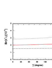
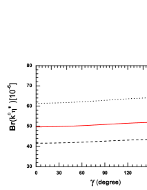
Figure 8: The $\gamma$ dependence of the branching ratios (in units of $10^{-6}$) of $B^{0}\to K^{0}\eta^{(\prime)}$ decays for $\omega_{b}=0.36$ GeV (dotted curve), 0.40 GeV (solid curve) and 0.44 GeV (dashed curve).

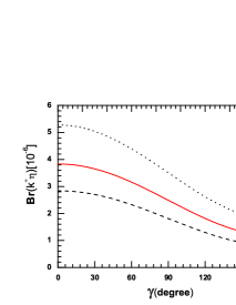
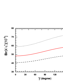
Figure 9: The $\gamma$ dependence of the branching ratios (in units of $10^{-6}$) of $B^{+}\to K^{+}\eta^{(\prime)}$ decays for $\omega_{b}=0.36$ GeV (dotted curve), 0.40 GeV (solid curve) and 0.44 GeV (dashed curve).

V.3 CP-violating asymmetries

Now we turn to the evaluations of the CP-violating asymmetries of $B\to K\eta^{(\prime)}$ decays in pQCD approach. For $B^{+}\to K^{+}\eta^{(\prime)}$ decays, the direct CP-violating asymmetries ${\cal A}_{CP}$ can be defined as:

$${\cal A}_{CP}^{dir}=\frac{|\overline{\cal M}_{f}|^{2}-|{\cal M}_{f}|^{2}}{|\overline{\cal M}_{f}|^{2}+|{\cal M}_{f}|^{2}},$$ (98)

Using Eq. (98), it is easy to calculate the direct CP-violating asymmetries for the considered decays, which are listed in Table 2. As a comparison, we also list currently available data hfag and the corresponding QCDF predictions npb675 .

Table 2: The pQCD predictions for the direct CP asymmetries in the NDR scheme (in units of $10^{-2}$), the QCDF predictions npb675 and the world average as given by HFAG hfag .

Mode	LO	$LO_{\rm{NLOWC}}$	+VC	+QL	+MP	NLO	Data	QCDF
${\cal A}_{CP}^{dir}(B^{\pm}\to K^{\pm}\eta)$	$9.3$	$10.3$	$31.1$	$7.8$	$7.6$	$-11.7$	$-27\pm 9$	$-18.9^{+29.0}_{-30.0}$
${\cal A}_{CP}^{dir}(B^{\pm}\to K^{\pm}\eta^{\prime})$	$-10.1$	$-7.3$	$-10.6$	$-5.9$	$-10.4$	$-6.2$	$1.6\pm 1.9$	$-9.0^{+10.6}_{-16.2}$

The NLO pQCD predictions for ${\cal A}_{CP}^{dir}(B^{+}\to K^{+}\eta^{(\prime)})$ (in unit of $10^{-2}$) with the major theoretical errors are

$${\cal A}_{CP}^{dir}(B^{\pm}\to K^{\pm}\eta) = -11.7^{+6.8}_{-9.6}(m_{s})^{+3.9}_{-4.2}(\gamma)^{+2.9}_{-5.6}(a^{\eta_{q}}_{2}),\quad$$

$${\cal A}_{CP}^{dir}(B^{\pm}\to K^{\pm}\eta^{\prime}) = -6.2^{+1.2}_{-1.1}(m_{s})^{+1.3}_{-1.0}(\gamma)^{+1.3}_{-1.0}(a^{\eta_{q}}_{2}),$$ (99)

where the dominant errors come from the variations of $m_{s}=130\pm 30$ MeV, $\gamma=60^{\circ}\pm 20^{\circ}$ and Gegenbauer coefficient $a^{\eta_{q}}_{2}=0.115\pm 0.115$, respectively.

As to the CP-violating asymmetries for the neutral decays $B^{0}\to K^{0}\eta^{(\prime)}$, the effects of $B^{0}-\bar{B}^{0}$ mixing should be considered. The CP-violating asymmetry of $B^{0}(\bar{B}^{0})\to K^{0}\eta^{(\prime)}$ decays are time dependent and can be defined as

$$A_{CP} \equiv \frac{\Gamma\left(\overline{B_{d}^{0}}(\Delta t)\to f_{CP}\right)-\Gamma\left(B_{d}^{0}(\Delta t)\to f_{CP}\right)}{\Gamma\left(\overline{B_{d}^{0}}(\Delta t)\to f_{CP}\right)+\Gamma\left(B_{d}^{0}(\Delta t)\to f_{CP}\right)}$$ (100)

$$= A_{CP}^{dir}\cos(\Delta m\Delta t)+A_{CP}^{mix}\sin(\Delta m\Delta t),$$

where $\Delta m$ is the mass difference between the two $B_{d}^{0}$ mass eigenstates, $\Delta t=t_{CP}-t_{tag}$ is the time difference between the tagged $B^{0}$ ($\overline{B}^{0}$) and the accompanying $\overline{B}^{0}$ ($B^{0}$) with opposite b flavor decaying to the final CP-eigenstate $f_{CP}$ at the time $t_{CP}$. The direct and mixing induced CP-violating asymmetries ${\cal A}_{CP}^{dir}$ ( or ${\cal A}_{f}$ in term of Belle Collaboration) and ${\cal A}_{CP}^{mix}$ can be written as

$${\cal A}_{CP}^{dir}={\cal A}_{f}=\frac{\left|\lambda_{CP}\right|^{2}-1}{1+|\lambda_{CP}|^{2}},\qquad{\cal A}_{CP}^{mix}={\cal S}_{f}=\frac{2Im(\lambda_{CP})}{1+|\lambda_{CP}|^{2}},$$ (101)

with the CP-violating parameter $\lambda_{CP}$

$$\lambda_{CP}\equiv\left(\frac{q}{p}\right)_{d}\cdot\frac{\langle f_{CP}|H_{eff}|\overline{B}^{0}\rangle}{\langle f_{CP}|H_{eff}|B^{0}\rangle}.$$ (102)

By integrating the time variable $t$, one finds the total CP asymmetries for $B^{0}\to K^{0}\eta^{(\prime)}$ decays,

$${\cal A}_{CP}^{tot}=\frac{1}{1+x^{2}}A_{CP}^{dir}+\frac{x}{1+x^{2}}A_{CP}^{mix},$$ (103)

where $x=\Delta m/\Gamma=0.775$ pdg2006 .

In Table 3, we show the pQCD predictions for the central values of the direct, mixing-induced and total CP asymmetries for $B^{0}\to K^{0}_{S}\eta^{(\prime)}$ decays, obtained by using the LO or NLO Wilson coefficients, and adding the vertex corrections, the quark loops, the magnetic penguin, or include all the mentioned NLO corrections, respectively.

Table 3: The pQCD predictions for the direct,mixing induced and total CP asymmetries (in units of $10^{-2}$) for $B^{0}\to K^{0}\eta^{(\prime)}$ decays, and the world average as given by HFAG hfag .

Mode	LO	$LO_{\rm{NLOWC}}$	+VC	+QL	+MP	NLO	Data
${\cal A}_{CP}^{dir}(B^{0}\to K^{0}_{S}\eta)$	$-4.2$	$-1.5$	$-11.2$	$-0.9$	$-1.9$	$-12.7$	$--$
${\cal A}_{CP}^{dir}(B^{0}\to K^{0}_{S}\eta^{\prime})$	$1.4$	$0.0$	$1.5$	$0.7$	$-0.1$	$2.3$	$9\pm 6$
${\cal A}_{CP}^{mix}(B^{0}\to K^{0}_{S}\eta)$	$61.6$	$67.3$	$64.4$	$66.9$	$67.9$	$61.9$	$--$
${\cal A}_{CP}^{mix}(B^{0}\to K^{0}_{S}\eta^{\prime})$	$64.6$	$63.5$	$63.4$	$63.2$	$63.2$	$62.7$	$61\pm 7$
${\cal A}_{CP}^{tot}(B^{0}\to K^{0}_{S}\eta)$	$27.2$	$31.7$	$24.2$	$31.9$	$31.7$	$22.1$	$--$
${\cal A}_{CP}^{tot}(B^{0}\to K^{0}_{S}\eta^{\prime})$	$32.1$	$30.8$	$31.7$	$31.0$	$30.5$	$31.8$	$--$

The NLO pQCD predictions for ${\cal A}_{CP}^{dir}(B^{0}\to K^{0}\eta^{(\prime)})$ and ${\cal A}_{CP}^{mix}(B^{0}\to K^{0}\eta^{(\prime)})$ (in unit of $10^{-2}$) with the major theoretical errors are

$${\cal A}_{CP}^{dir}(B^{0}\to K^{0}_{S}\eta) = -12.7\pm 4.1(m_{s})^{+3.2}_{-1.5}(\gamma)^{+3.2}_{-6.7}(a^{\eta_{q}}_{2}),$$

$${\cal A}_{CP}^{dir}(B^{0}\to K^{0}_{S}\eta^{\prime}) = 2.3^{+0.5}_{-0.4}(m_{s})^{+0.3}_{-0.6}(\gamma)^{+0.2}_{-0.1}(a^{\eta_{q}}_{2}),$$

$${\cal A}_{CP}^{mix}(B^{0}\to K^{0}_{S}\eta) = 61.9^{+35.8}_{-65.0}(\gamma)^{+35.3}_{-64.3}(\alpha),$$

$${\cal A}_{CP}^{mix}(B^{0}\to K^{0}_{S}\eta^{\prime}) = 62.7^{+35.5}_{-65.0}(\gamma)^{+35.4}_{-64.7}(\alpha),,$$ (104)

where the dominant errors come from the variations of $m_{s}=130\pm 30$ MeV, $\gamma=60^{\circ}\pm 20^{\circ}$, $\alpha=100^{\circ}\pm 20^{\circ}$, and the Gegenbauer coefficient $a^{\eta_{q}}_{2}=0.115\pm 0.115$, respectively.

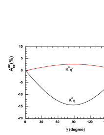
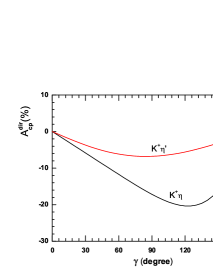
Figure 10: The NLO pQCD predictions for direct CP asymmetries (in percentage) of $B^{0}\to K^{0}_{S}\eta^{(\prime)}$ and $B^{\pm}\to K^{\pm}\eta^{(\prime)}$ decays.

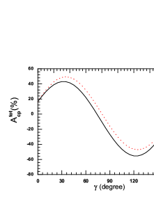
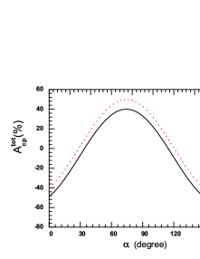
Figure 11: The $\gamma$-dependence (a) and the $\alpha$-dependence (b) of the total CP-asymmetries of $B^{0}\to K^{0}_{S}\eta$ (solid curve) and $B^{0}\to K^{0}_{S}\eta^{\prime}$ (dotted curve) decays.

In Fig. 10, we shown the $\gamma$-dependence of the pQCD predictions for direct CP-violating asymmetries of $B^{0}\to K^{0}_{S}\eta^{(\prime)}$ and $B^{+}\to K^{+}\eta^{(\prime)}$ decays. In Fig. 11, we shown the $\alpha$-dependence of the total CP-violating asymmetries for $B^{0}\to K^{0}_{S}\eta$ (solid curve) and $B^{0}\to K^{0}_{S}\eta^{\prime}$ (dotted curve), respectively.

From the pQCD predictions and currently available experimental measurements for the CP violating asymmetries of the four $B\to K\eta^{(\prime)}$ decays, one can see the following points:

• (a) For $B^{+}\to K^{+}\eta$ decay, the measured direct CP asymmetry is 3 standard deviation from zero. The LO pQCD prediction changed its sign and become consistent with the measured one due to the inclusion of NLO contributions.

• (b) For ${\cal A}_{CP}^{dir}(B^{\pm}\to K^{\pm}\eta^{\prime})$, the pQCD prediction is changed from $-10\%$ to $-6\%$ due to the inclusion of NLO contributions, which is consistent with the measured zero result within one standard deviation.

• (c) For $B^{0}\to K^{0}\eta^{(\prime)}$ decay, the effects of NLO contributions to their CP asymmetries are rather small, as can be seen from the numerical results as given in Table 3.

• (d) For neutral $B^{0}\to K^{0}\eta^{(\prime)}$ decays, the PQCD predictions are ${\cal A}_{CP}^{dir}(B^{0}\to K^{0}_{S}\eta^{\prime})\approx 2.3\%$ and ${\cal A}_{CP}^{mix}(B^{0}\to K^{0}_{S}\eta^{\prime})\approx 63\%$, which agree very well with the data: $(9\pm 6)\%$ and $(61\pm 7)\%$. This means that the deviation $\Delta S=-\eta_{f}S_{f}-\sin 2\beta$ for $B^{0}\to K^{0}\eta^{\prime}$ decay is also very small in the pQCD approach.

VI summary

In this paper, we calculated the branching ratios and CP-violating asymmetries of $B^{+}\to K^{+}\eta^{(\prime)}$ and $B^{0}\to K^{0}\eta^{(\prime)}$ decays in the pQCD approach. The partial NLO contributions considered here include: QCD vertex corrections, the quark-loops and the chromo-magnetic penguins.

From our calculations and phenomenological analysis, we found the following results:

• (a) The pQCD predictions for the form factors of $B\to\eta^{(\prime)}$ and $B\to K$ transitions are

  $$F^{B\to\eta}_{0}(q^{2}=0) = 0.21\pm 0.03(\omega_{b}),$$

  $$F^{B\to\eta^{\prime}}_{0}(q^{2}=0) = 0.17\pm 0.03(\omega_{b}),$$

  $$F^{B\to K}_{0}(q^{2}=0) = 0.37^{+0.06}_{-0.05}(\omega_{b}),$$ (105)

  for $\omega_{b}=0.40\pm 0.04$ GeV, which agree well with those obtained in QCD sum rule.

• (b) For branching ratios, the NLO pQCD predictions (in unit of $10^{-6}$) are

  $$Br(B^{+}\to K^{+}\eta) = 3.2^{+3.2}_{-1.8},$$

  $$Br(B^{\pm}\to K^{\pm}\eta^{\prime}) = 51.0^{+18.0}_{-10.9},$$

  $$Br(B^{0}\to K^{0}\eta) = 2.1^{+2.6}_{-1.5},$$

  $$Br(B^{0}\to K^{0}\eta^{\prime}) = 50.3^{+16.8}_{-10.6},$$ (106)

  where the individual theoretical errors have been added in quadrature. The decay amplitude $B\to K\eta_{q}$ and $B\to K\eta_{s}$ interfere constructively for $B\to K\eta^{\prime}$ decays, but destructively for $B\to K\eta$ decays. The NLO contributions in the pQCD approach, furthermore, can provide a $70\%$ enhancement to $Br(B\to K\eta^{\prime})$, but a $30\%$ reduction to $Br(B\to K\eta)$. The large branching ratio of $B\to K\eta^{\prime}$ decays, as well as the large disparity $Br(B\to K\eta^{\prime})\gg Br(B\to K\eta)$ can therefore be understood naturally.

• (c) The pQCD predictions for the CP asymmetries of $B\to K\eta^{(\prime)}$ decays are consistent with currently available data. For neutral $B^{0}\to K^{0}\eta^{(\prime)}$ decays, for example, the PQCD predictions are ${\cal A}_{CP}^{dir}(B^{0}\to K^{0}_{S}\eta^{\prime})\approx 2.3\%$ and ${\cal A}_{CP}^{mix}(B^{0}\to K^{0}_{S}\eta^{\prime})\approx 63\%$, which agree very well with the measured values of $(9\pm 6)\%$ and $(61\pm 7)\%$, respectively.

• (d) In this paper, only the partial NLO contributions have been taken into account. We think that they are the dominant part of the whole NLO corrections. To achieve a complete NLO calculations in the pQCD approach, the still missing pieces from the emission diagrams, hard-spectator and annihilation diagrams, should be evaluated as soon as possible.

Appendix A Related Functions

We show here the function $h_{i}$’s, coming from the Fourier transformations of the hard kernel $H^{(0)}(x_{i},b_{i})$,

$$h_{e}(x_{1},x_{2},b_{1},b_{2}) = K_{0}\left(\sqrt{x_{1}x_{2}}m_{B}b_{1}\right)\left[\theta(b_{1}-b_{2})K_{0}\left(\sqrt{x_{2}}m_{B}b_{1}\right)I_{0}\left(\sqrt{x_{2}}m_{B}b_{2}\right)\right.$$ (107)

$$\;\left.+\theta(b_{2}-b_{1})K_{0}\left(\sqrt{x_{2}}m_{B}b_{2}\right)I_{0}\left(\sqrt{x_{2}}m_{B}b_{1}\right)\right]S_{t}(x_{2}),$$

$$h_{a}(x_{2},x_{3},b_{2},b_{3}) = K_{0}\left(i\sqrt{(1-x_{2})x_{3}}m_{B}b_{2}\right)\left[\theta(b_{3}-b_{2})K_{0}\left(i\sqrt{x_{3}}m_{B}b_{3}\right)I_{0}\left(i\sqrt{x_{3}}m_{B}b_{2}\right)\right.$$ (108)

$$\;\;\;\;\left.+\theta(b_{2}-b_{3})K_{0}\left(i\sqrt{x_{3}}m_{B}b_{2}\right)I_{0}\left(i\sqrt{x_{3}}m_{B}b_{3}\right)\right]S_{t}(x_{3}),$$

$$h_{f}(x_{1},x_{2},x_{3},b_{1},b_{3}) = \biggl{\{}\theta(b_{1}-b_{3})\mathrm{K}_{0}(M_{B}\sqrt{x_{1}x_{2}}b_{1})\mathrm{I}_{0}(M_{B}\sqrt{x_{1}x_{2}}b_{3})$$ (109)

$$+ \theta(b_{3}-b_{1})\mathrm{K}_{0}(M_{B}\sqrt{x_{1}x_{2}}b_{3})\mathrm{I}_{0}(M_{B}\sqrt{x_{1}x_{2}}b_{1})\biggr{\}}$$

$$\cdot\left(\begin{matrix}\frac{\pi i}{2}\mathrm{H}_{0}(\sqrt{(x_{2}(x_{3}-x_{1}))}M_{B}b_{3}),&\text{for}\quad x_{1}-x_{3}<0\\ \mathrm{K}_{0}^{(1)}(\sqrt{(x_{2}(x_{1}-x_{3})}M_{B}b_{3}),&\text{for}\quad x_{1}-x_{3}>0\end{matrix}\right),$$

$$h_{f}^{3}(x_{1},x_{2},x_{3},b_{1},b_{3}) = \biggl{\{}\theta(b_{1}-b_{3})\mathrm{K}_{0}(i\sqrt{(1-x_{2})x_{3}}b_{1}M_{B})\mathrm{I}_{0}(i\sqrt{(1-x_{2})x_{3}}b_{3}M_{B})$$ (110)

$$+ (\theta(b_{3}-b_{1})\mathrm{K}_{0}(i\sqrt{(1-x_{2})x_{3}}b_{3}M_{B})\mathrm{I}_{0}(i\sqrt{(1-x_{2})x_{3}}b_{1}M_{B})\biggr{\}}$$

$$\cdot\left(\begin{matrix}\mathrm{K}_{0}(M_{B}\sqrt{(x_{1}-x_{3})(1-x_{2})}b_{1}),&\text{for}\quad x_{1}-x_{3}>0\\ \frac{\pi i}{2}\mathrm{H}_{0}^{(1)}(M_{B}\sqrt{(x_{3}-x_{1})(1-x_{2})}b_{1}),&\text{for}\quad x_{1}-x_{3}<0\end{matrix}\right),$$

$$h_{f}^{4}(x_{1},x_{2},x_{3},b_{1},b_{2}) = \biggl{\{}\theta(b_{1}-b_{3})\mathrm{K}_{0}(i\sqrt{(1-x_{2})x_{3}}b_{1}M_{B})\mathrm{I}_{0}(i\sqrt{(1-x_{2})x_{3}}b_{3}M_{B})$$ (111)

$$+ \theta(b_{3}-b_{1})\mathrm{K}_{0}(i\sqrt{(1-x_{2})x_{3}}b_{3}M_{B})\mathrm{I}_{0}(i\sqrt{(1-x_{2})x_{3}}b_{1}M_{B})\biggr{\}}$$

$$\cdot\left(\begin{matrix}\mathrm{K}_{0}(M_{B}F_{1}b_{1}),&\text{for}\quad F_{1}^{2}>0\\ \frac{\pi i}{2}\mathrm{H}_{0}^{(1)}(M_{B}\sqrt{|F_{1}^{2}|}b_{1}),&\text{for}\quad F_{1}^{2}<0\end{matrix}\right),$$

where $J_{0}$ is the Bessel function and $K_{0}$, $I_{0}$ are modified Bessel functions with $K_{0}(-ix)=-(\pi/2)Y_{0}(x)+i(\pi/2)J_{0}(x)$, and $F_{(1)}$’s are defined by

$$F^{2}_{(1)} = 1-x_{2}(1-x_{1}-x_{3}).$$ (112)

The threshold resummation form factor $S_{t}(x_{i})$ is adopted from Ref. kurimoto . It has been parameterized as

$$S_{t}(x)=\frac{2^{1+2c}\Gamma(3/2+c)}{\sqrt{\pi}\Gamma(1+c)}[x(1-x)]^{c},$$ (113)

where the parameter $c=0.3$. This function is normalized to unity.

The evolution factors $E^{(\prime)}_{e}$, and $E^{(\prime)}_{a}$, appeared in the decay amplitudes are given by

$$E_{e}(t) = \alpha_{s}(t)\exp[-S_{ab}(t)],$$

$$E_{e}^{\prime}(t) = \alpha_{s}(t)\exp[-S_{cd}(t)]|_{b_{2}=b_{1}},$$

$$E_{a}^{\prime}(t) = \alpha_{s}(t)\exp[-S_{ef}(t)]|_{b_{2}=b_{3}},$$

$$E_{a}(t) = \alpha_{s}(t)\exp[-S_{gh}(t)].$$ (114)

The Sudakov factors used in the text are defined as

$$S_{ab}(t) = s\left(x_{1}m_{B}/\sqrt{2},b_{1}\right)+s\left(x_{2}m_{B}/\sqrt{2},b_{2}\right)+s\left((1-x_{2})m_{B}/\sqrt{2},b_{2}\right)$$ (115)

$$-\frac{1}{\beta_{1}}\left[\ln\frac{\ln(t/\Lambda)}{-\ln(b_{1}\Lambda)}+\ln\frac{\ln(t/\Lambda)}{-\ln(b_{2}\Lambda)}\right],$$

$$S_{cd}(t) = s\left(x_{1}m_{B}/\sqrt{2},b_{1}\right)+s\left(x_{2}m_{B}/\sqrt{2},b_{1}\right)+s\left((1-x_{2})m_{B}/\sqrt{2},b_{1}\right)$$ (116)

$$+s\left(x_{3}m_{B}/\sqrt{2},b_{3}\right)+s\left((1-x_{3})m_{B}/\sqrt{2},b_{3}\right)$$

$$-\frac{1}{\beta_{1}}\left[2\ln\frac{\ln(t/\Lambda)}{-\ln(b_{1}\Lambda)}+\ln\frac{\ln(t/\Lambda)}{-\ln(b_{3}\Lambda)}\right],$$

$$S_{ef}(t) = s\left(x_{1}m_{B}/\sqrt{2},b_{1}\right)+s\left(x_{2}m_{B}/\sqrt{2},b_{3}\right)+s\left((1-x_{2})m_{B}/\sqrt{2},b_{3}\right)$$ (117)

$$+s\left(x_{3}m_{B}/\sqrt{2},b_{3}\right)+s\left((1-x_{3})m_{B}/\sqrt{2},b_{3}\right)$$

$$-\frac{1}{\beta_{1}}\left[\ln\frac{\ln(t/\Lambda)}{-\ln(b_{1}\Lambda)}+2\ln\frac{\ln(t/\Lambda)}{-\ln(b_{2}\Lambda)}\right],$$

$$S_{gh}(t) = s\left(x_{2}m_{B}/\sqrt{2},b_{2}\right)+s\left(x_{3}m_{B}/\sqrt{2},b_{3}\right)+s\left((1-x_{2})m_{B}/\sqrt{2},b_{2}\right)$$ (118)

$$+ s\left((1-x_{3})m_{B}/\sqrt{2},b_{3}\right)-\frac{1}{\beta_{1}}\left[\ln\frac{\ln(t/\Lambda)}{-\ln(b_{3}\Lambda)}+\ln\frac{\ln(t/\Lambda)}{-\ln(b_{2}\Lambda)}\right],$$

where the function $s(q,b)$ are defined in the Appendix A of Ref.luy01 . The scale $t_{i}$’s in the above equations are chosen as

$$t_{a} = {\rm max}(\sqrt{x_{2}}m_{B},\sqrt{x_{1}x_{2}}m_{B},1/b_{1},1/b_{2})\;,$$

$$t_{a}^{\prime} = {\rm max}(\sqrt{x_{1}}m_{B},\sqrt{x_{1}x_{2}}m_{B},1/b_{1},1/b_{2})\;,$$

$$t_{b} = {\rm max}(\sqrt{x_{2}|1-x_{3}-x_{1}|}m_{B},\sqrt{x_{1}x_{2}}m_{B},1/b_{1},1/b_{3})\;,$$

$$t_{b}^{\prime} = {\rm max}(\sqrt{x_{2}|x_{3}-x_{1}|}m_{B},\sqrt{x_{1}x_{2}}m_{B},1/b_{1},1/b_{3})\;,$$

$$t_{c} = {\rm max}(\sqrt{(1-x_{2})x_{3}}m_{B},\sqrt{|x_{1}-x_{3}|(1-x_{2})}m_{B},1/b_{1},1/b_{3})\;,$$

$$t_{c}^{\prime} = {\rm max}(\sqrt{|1-x_{2}(1-x_{3}-x_{1})|}m_{B},\sqrt{(1-x_{2})x_{3}}m_{B},1/b_{1},1/b_{3})\;,$$

$$t_{d} = {\rm max}(\sqrt{(1-x_{2})x_{3}}m_{B},\sqrt{(1-x_{2})}m_{B},1/b_{2},1/b_{3})\;,$$

$$t_{d}^{\prime} = {\rm max}(\sqrt{(1-x_{2})x_{3}}m_{B},\sqrt{x_{3}}m_{B},1/b_{2},1/b_{3})\;.$$ (119)

References

- (1) B.H. Behrens, CLEO Collaboration, Phys. Rev. Lett. 80, 3710 (1998).
- (2) E. Barberio et al., (Heavy Flavor Averaging Group), arXiv:0704.3575 [hep-ex] and online update at http://www.slac.stanford.edu/xorg/hfag
- (3) P. Chang et al., (Belle Collaboration), Phys. Rev. D 71, 091106(R) (2005); K.-F. Chen et al., (Belle Collaboration), Phys. Rev. Lett. 98, 031802 (2007); B. Aubert et al., (BaBar Collaboration), Phys. Rev. D 76, 031103(R) (2007); Phys. Rev. Lett. 98, 031801 (2007).
- (4) H.J. Lipkin, Phys. Lett. B 254, 247 (1991).
- (5) Y. Grossman and M.P. Worah, Phys. Lett. B 395, 241 (1997).
- (6) D. Atwood and A. Soni, Phys. Lett. B 405, 150 (1997); W.S. Hou and B. Tseng, Phys. Rev. Lett. 80, 434 (1998).
- (7) F. Yuan and K.T. Chao, Phys. Rev. D 56, R2495 (1997); I. Haperin and A. Zhitnitsky, Phys. Rev. D 56, 7247 (1997); Phys. Rev. Lett. 80, 538 (1998).
- (8) A. Ali, J. Chay, C. Greub, and P. Ko, Phys. Lett. B 424, 161 (1998).
- (9) D.S. Du,C.S. Kim, Y.D. Yang, Phys. Lett. B 426, 133 (1998).
- (10) M.Z. Yang and Y.D. Yang, Nucl. Phys. B 609, 469 (2001).
- (11) M.R. Ahmady, E. Kou, A. Sugamoto, Phys. Rev. D 58, 014015 (1998).
- (12) A.L. Kagan and A.A. Petrov, hep-ph/9707354; S. Khalil and E. Kou, Phys. Rev. Lett. 91, 241602 (2003).
- (13) G.R. Lu, Z.J. Xiao, H.K. Guo and L.X. Lü, J. Phys. G 25, L85 (1999); Z.J. Xiao, K.T. Chao and C.S. Li, Phys. Rev. D 65, 114021(2002); Z.J. Xiao and W.J. Zou, Phys. Rev. D 70, 094008 (2004).
- (14) M. Beneke and M. Neubert, Nucl. Phys. B 651, 225 (2003).
- (15) M. Beneke and M. Neubert, Nucl. Phys. B 675, 333 (2003).
- (16) E. Kou and A. Sanda, Phys. Lett. B 525, 240 (2002).
- (17) M. Beneke, G. Buchalla, M. Neubert, and C.T. Sachrajda, Phys. Rev. Lett. 83, 1914 (1999);
- (18) H.N. Li, Prog. Part. Nucl. Phys. 51, 85 (2003) and references therein.
- (19) T. Feldmann, P. Kroll, and B. Stech, Phys. Rev. D 58, 114006 (1998); T. Feldmann, Int. J. Mod. Phys. A15, 159 (2000).
-
(20)
R. Escribano and J.M. Frere, J. High Energy Phys. 0506 (2005) 029;
J. Schechter, A. Subbaraman and H. Weigel, Phys. Rev. D 48, 339 (1993). - (21) Y.Y. Charng, T. Kurimoto, and H.N. Li, Phys. Rev. D 74, 074024 (2006).
- (22) P. Ball and G.W. Jones, J. High Energy Phys. 0708 (2007) 025.
- (23) A. G. Akeroyd, C.H. Chen, and C.Q. Geng, Phys. Rev. D 75, 054003 (2007).
- (24) J.F. Hsu, Y.Y. Charng, and H.N. Li, arXiv:0711.4987 [hep-ph].
- (25) H.N. Li, S. Mishima, A.I. Sanda, Phys. Rev. D 72, 114005 (2005).
- (26) M. Beneke, Phys. Lett. B 620, 143 (2005); G. Buchalla et al., J. High Energy Phys. 0509 (2005)074; H.Y. Cheng, C.K. Chua and A. Soni, Phys. Rev. D 72, 014006 (2005).
- (27) A.R. Williamson and J. Zupan, Phys. Rev. D 74 , 014003 (2006).
- (28) Y.-Y. Keum, H.N. Li and A.I. Sanda, Phys. Rev. D 63, 054008 (2001).
- (29) C.D. Lü, K. Ukai and M.Z. Yang, Phys. Rev. D 63, 074009 (2001).
- (30) X. Liu, H.S. Wang, Z.J. Xiao, L.B. Guo, and C.D. Lü, Phys. Rev. D 73, 074002 (2006); H.S. Wang, X. Liu, Z.J. Xiao, L.B. Guo, and C.D. Lü, Nucl. Phys. B 738, 243 (2006).
- (31) Z.J. Xiao, D.Q. Guo, and X.F. Chen, Phys. Rev. D 75, 014018 (2007); D.Q. Guo, Z.J. Xiao, and X.F. Chen, Phys. Rev. D 75, 054003 (2007); X.F. Chen, D.Q. Guo, and Z.J. Xiao, Eur. Phys. J. C 50, 363 (2007).
- (32) G. Buchalla, A.J. Buras, and M.E. Lautenbacher, Rev. Mod. Phys. 68, 1125 (1996).
- (33) M. Beneke, Nucl.Phys.B(Proc.Suppl.) 170, 57 (2007).
- (34) Z.Q. Zhang and Z.J. Xiao, arXiv: 0807.2022 [hep-ph].
- (35) Z.Q. Zhang and Z.J. Xiao, arXiv: 0807.2024 [hep-ph].
- (36) C.D. Lü, M.Z. Yang, Eur. Phys. J. C 28, 515 (2003).
- (37) P. Ball, V.M. Braun, Y. Koike, and K. Tanaka, Nucl. Phys. B 529, 323 (1998); P. Ball, J. High Energy Phys. 9809 (1998) 005; J. High Energy Phys. 9901 (1999) 010; P. Ball and R. Zwicky, Phys. Rev. D 71, 014015 (2005); J. High Energy Phys. 0604 (2006) 046.
- (38) S. Mishima and A.I. Sanda, Prog. Theor. Phys. 110, 549 (2003).
- (39) M. Bander, D. Silverman and A. Soni, Phys. Rev. Lett. 43, 242 (1979); J.M. Gerard and W.S. Hou, Phys. Rev. D 43, 2909 (1991).
- (40) Particle Data Group, W.-M. Yao et al., J. Phys. G 33, 1 (2006).
- (41) T. Kurimoto, H.N. Li, A.I. Sanda, Phys. Rev. D 65 (2002) 014007.