Dirac-point engineering and topological phase transitions
in honeycomb optical lattices

Abstract

We study the electronic structure and the phase diagram of non-interacting fermions confined to hexagonal optical lattices. In the first part, we compare the properties of Dirac points arising in the eigenspectrum of either honeycomb or triangular lattices. Numerical results are complemented by analytical equations for weak and strong confinements. In the second part we discuss the phase diagram and the evolution of Dirac points in honeycomb lattices applying a tight-binding description with arbitrary nearest-neighbor hoppings. With increasing asymmetry between the hoppings the Dirac points approach each other. At a critical asymmetry the Dirac points merge to open an energy gap, thus changing the topology of the eigenspectrum. We analyze the trajectory of the Dirac points and study the density of states in the different phases. Manifestations of the phase transition in the temperature dependence of the specific heat and in the structure factor are discussed.

I Introduction

The isolation of a single layer of grapheneNovoselov et al. (2004), which is a two-dimensional honeycomb lattice of carbon atoms, has attracted considerable attention, both for its basic interest and because it may pave the way to carbon-based electronics. The low energy electronic properties are described by the massless Dirac equation, which causes many anomalies with respect to semiconductor physicsCastro Neto et al. (2007); Geim and Novoselov (2007); Beenakker (2007). Close to half-filling, the band structure near the Fermi energy is given by two degenerate Dirac cones, and the centers of these cones (called Dirac points) are located at the two distinct K-points of the first Brillouin zone. A first experimental validation of the relativistic band structure was the measurement of the anomalous sequencing of the Quantum Hall plateausZhang et al. (2005); Novoselov et al. (2005).

In graphene there is little room to tune system parameters such as the interaction strength or the hopping amplitudes, which prevents a systematic study of its phase diagram. In contrast for cold fermionic atoms confined in honeycomb optical latticesGrynberg et al. (1993) the parameters are highly tunable and many of the theoretically predicted phases might be realized there. Recent theoretical works on honeycomb lattices have studied a topological phase transition in the single particle spectrum which is due either to asymmetric hopping energiesZhu et al. (2007), or to a Kekulé distortion of the hoppingsHou et al. (2007); Herbut (2007), or to the application of an ac electric fieldZhang et al. (2008). Further work on honeycomb optical lattices has dealt with the realization of the anomalous Hall and the Spin Hall effectsDudarev et al. (2004), the Wigner crystallization of $\pi$-bandsWu and Das Sarma (2007); Wu et al. (2007), or with the Quantum Hall effect without Landau levelsWu (2008); Shao et al. (2008); Haldane (1988). Finally, we note recent theoretical work on the appearance and manifestation of Dirac cones in the band structure of triangular photonic crystalsHaldane and Raghu (2008); Raghu and Haldane (2006); Sepkhanov et al. (2008).

There are two main purposes of this work. The first one is to compare the Dirac points present in the lower lying bands of triangular and honeycomb lattices. Therefore we first discuss in section II the potential landscape of these lattices. Then, in section III we discuss the Dirac cones appearing in both lattice types and derive analytical results within the nearly-free-particle and tight-binding limits. The second main goal of this work is to analyze in detail the topological phase transition in honeycomb lattices with asymmetric hopping energiesZhu et al. (2007). In section IV, the evolution of the Dirac points and the resulting phase diagram for the honeycomb lattice as a function of the relative tunnel couplings are studied within the tight-binding limit . The density of states for the different phases is derived in section V. Experimental signatures of the phase transition such as the structure factor and the temperature dependence of the specific heat are explained in section VI. Finally, we discuss the topological structure of the phase transition in section VII. Some technical derivations are left to the Appendices.

II Potential landscapes

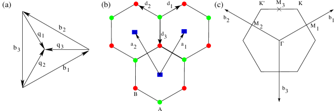
Figure 1: (a) Three traveling lasers with wavevectors ${\bf q}_{i}$ interfere and build up the hexagonal lattice with reciprocal unit vectors ${\bf b}_{1},{\bf b}_{2}$, and ${\bf b}_{3}=-({\bf b}_{1}+{\bf b}_{2})$. (b) Unit cell in real space spanned by the unit vectors ${\bf a}_{1},{\bf a}_{2}$. For triangular lattices the minima are located at the center of the hexagons, while for symmetric honeycomb lattices minima lie at the $A$ and $B$ sites. (c) Unit cell in reciprocal space (first Brillouin zone) indicating the position of the symmetry points $\Gamma,{\rm M_{1},M_{2},M_{3}}$ and the K-points.

We consider the optical lattice that was experimentally realized by Grynberg et al. Grynberg et al. (1993). It is created by three interfering traveling laser beams. The corresponding wave vectors are in the $x-y$ plane and form equal angles between them, as illustrated in Fig. 1a. For simplicity we assume the polarization of the beams to be perpendicular to the plane, although the confining potential is independent of the polarization for large enough detuningDudarev et al. (2004).

The amplitude of the total electric field (polarized in the $z$-direction) and the light intensity can then be written

$$E({\bf r}) = \sum_{j}E_{j}\exp(i{\bf q}_{j}\cdot{\bf r})$$ (1)

$$I({\bf r}) = |E({\bf r})|^{2}=E_{1}^{2}+E_{2}^{2}+E_{3}^{2}+2E_{1}E_{2}\cos({\bf b}_{3}\cdot{\bf r})+2E_{2}E_{3}\cos({\bf b}_{1}\cdot{\bf r})+2E_{3}E_{1}\cos({\bf b}_{2}\cdot{\bf r})\;.$$ (2)

As illustrated in Fig. 1a ${\bf b}_{1}={\bf q}_{2}-{\bf q}_{3}$ plus cyclic permutations. We note that the system is essentially insensitive to phase drifts between the lasers, since these just shift the lattice without changing the potential landscape. We can therefore assume $E_{i}>0$ without loss of generality.

The optical confining potential $V({\bf r})$ is proportional to the intensity of the laser field and the proportionality factor is positive (negative) if the laser frequencies are blue (red) detuned with respect to the transition frequency of the atoms. Up to a constant the confinement is given by

$$V({\bf r}) = \sum_{j}V_{j}\cos({\bf b}_{j}\cdot{\bf r}),$$ (3)

with $V_{1}\propto E_{2}E_{3}$ plus cyclic permutations and $V_{j}>0$ ($V_{j}<0$) for blue (red) detuning.

The potential $V({\bf r})$ has an underlying triangular Bravais lattice, whose lattice spacing $a$ is determined by the wavelength of the traveling lasers $a=4\pi/3q=2\lambda/3$. The unit vectors for real and reciprocal lattices are given by:

$${\bf a}_{1} = \frac{a}{2}\left(\begin{array}[]{c}1\\ \sqrt{3}\end{array}\right)\,;\quad{\bf a}_{2}=\frac{a}{2}\left(\begin{array}[]{c}-1\\ \sqrt{3}\end{array}\right)\,;\quad{\bf b}_{1}=\frac{2\pi}{\sqrt{3}a}\left(\begin{array}[]{c}\sqrt{3}\\ 1\end{array}\right)\,;\quad{\bf b}_{2}=\frac{2\pi}{\sqrt{3}a}\left(\begin{array}[]{c}-\sqrt{3}\\ 1\end{array}\right)\quad$$ (12)

with ${\bf b}_{i}\cdot{\bf a}_{j}=2\pi\delta_{ij}$. The unit cells of both reciprocal and real space can be chosen of honeycomb form as shown in Figs 1b and c.

In the case of red detuning, the potential minima lie at the centers of the hexagons thus forming a triangular lattice for all values of $V_{j}<0$. If the lasers are blue detuned and their intensities are equal, then the minima of the potential $V({\bf r})$ are located at the vertices of the honeycombs while there is a maximum of the potential at the center of each honeycomb, see Fig. 1b. If the intensities $V_{j}$ become different (i.e. the electric field amplitudes $E_{j}$ begin to be different), the two minima per unit cell approach each other until they merge for strong asymmetries, namely, when $|E_{1}-E_{2}|>E_{3}$ or $E_{3}>E_{1}+E_{2}$. Thus the potential $V({\bf r})$ (3) has two minima per unit cell for $|E_{1}-E_{2}|<E_{3}<E_{1}+E_{2}$. It is evident from Eq. (3) that the potential $V({\bf r})$ has inversion symmetry, which is crucial for the stability of the Dirac pointsMañes et al. (2007). The position of the minima are given by ${\bf r}=\pm{\bf r}_{\rm min}$ with:

$${\bf r}_{\rm min}=\left(\begin{array}[]{c}\frac{a}{2\pi}\;\text{sgn}(E_{2}-E_{1})\arccos\left(\frac{E_{1}+E_{2}}{E_{3}}\sqrt{\frac{E_{3}^{2}-(E_{2}-E_{1})^{2}}{4E_{1}E_{2}}}\right)\\ \frac{a\sqrt{3}}{2\pi}\;\arccos\left(-\sqrt{\frac{E_{3}^{2}-(E_{2}-E_{1})^{2}}{4E_{1}E_{2}}}\right)\end{array}\right)$$ (15)

We will show in section IV that the energy dispersion $E_{\bf k}$ calculated within the tight-binding approximation has the same structure as the potential $V({\bf r})$. The analog of the motion of the potential minima for the case of the energy spectrum is the evolution of the Dirac points (24), which will finally merge, causing a topological phase transition from a semimetal to an insulator.

III Symmetric lattices

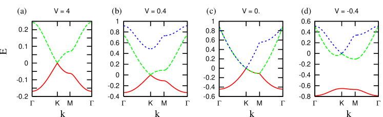
Figure 2: Band structure for the symmetric lattice ($V_{1}=V_{2}=V_{3}=V$) along characteristic lines of the first Brillouin zone for various values of $V$. Symmetry points are explained in Fig. 1c. The energy of Dirac point is set to 0 and the unit of energy is $(\hbar^{2}/2m)(4\pi^{2}/a^{2})$.

Because of periodic translational invariance, the crystal momentum is conserved and the eigenspectrum of a particle moving in the potential $V({\bf r})$ of Eq. (3) is most conveniently calculated in Fourier space. The eigenfunctions are thus written as $\psi_{\bf q}({\bf r})=\sum_{m,n}c_{{\bf q}-{\bf G}_{mn}}\exp(i({\bf q}-{\bf G}_{mn})\cdot{\bf r})$, where ${\bf q}$ is restricted to be in the first Brillouin zone, ${\bf G}_{mn}=m{\bf b}_{1}+n{\bf b}_{2}$ denotes a general reciprocal lattice vector, and the potential is written as $V({\bf r})=\sum_{mn}V_{mn}\exp(i{\bf G}_{mn}\cdot{\bf r})$ where $V_{mn}=\frac{1}{2}\left[V_{3}(\delta_{m,1}\delta_{n,1}+\delta_{m,-1}\delta_{n,-1})+V_{1}\delta_{n,0}(\delta_{m,1}+\delta_{m,-1})+V_{2}\delta_{m,0}(\delta_{n,1}+\delta_{n,-1})\right]$ are the Fourier components of the potential. Due to inversion symmetry of the lattice $V_{mn}=V_{-m,-n}$.

For each ${\bf q}$ the Fourier components $c_{{\bf q}-{\bf G}_{mn}}$ form a vector ${\bf v}_{\bf q}$, where each entry is labeled by a specific pair of integers $({\bf v}_{\bf q})_{mn}=c_{{\bf q}-{\bf G}_{mn}}$. The Schrödinger equation then reduces to a set of linear equations for each ${\bf v}_{\bf q}$ given by:

$${\bf M}_{\bf q}{\bf v}_{\bf q} = E_{\bf q}{\bf v}_{\bf q}$$ (16)

$$({\bf M}_{\bf q})_{(m_{1},n_{1}),(m_{2},n_{2})} = \delta_{m_{1},m_{2}}\delta_{n_{1},n_{2}}E^{0}_{{\bf q}-{\bf G}_{m_{1},n_{1}}}+V_{m_{1}-m_{2},n_{1}-n_{2}}$$

where $E^{0}_{{\bf q}}=\hbar^{2}q^{2}/2m$ denotes the kinetic energy.

Figure 2 shows the band structure for symmetric potentials $V_{1}=V_{2}=V_{3}=V$ for various confinement strengths $V$. Most importantly, we note that, both for triangular and honeycomb lattices, some pairs of bands touch at the K-points and in the vicinity of those touching points the band structure is given by cones, which are called Dirac cones because of the similarity to the relativistic energy dispersion.

There are however important differences between both cases. For the honeycomb lattice the first pair of Dirac points (located at $\pm{\bf K}$) arises due to the touching of the two lowest bands. Furthermore, the Fermi surface in the relevant energy interval is exclusively determined by these Dirac cones, leading in particular to a vanishing density of states at complete filling of the lowest band.

By contrast, for a triangular lattice the first pair of Dirac points is caused by the touching between the second and third band. Since these bands are also degenerate at the $\Gamma$ point, the Dirac points are not isolated but resonate with a continuous band that dominates the density of states in the energy regime of the Dirac cones. Furthermore, the filling factor (number of atoms per unit cell) at which the Fermi energy coincides with the Dirac point is not an integer, also in contrast to the honeycomb lattice.

The formation of the Dirac cone can be derived within the nearly-free-particle approximation, where the potential is treated perturbatively as shown in Appendix A. The distinction between honeycomb and triangular lattices is however better appreciated in the tight-binding regime, where the Hamiltonian is written in terms of Wannier states, each localized at a potential minimum as shown in Appendix B.

In the following we concentrate on the honeycomb lattice within the tight-binding approximation.

IV Dirac points in asymmetric honeycomb lattices

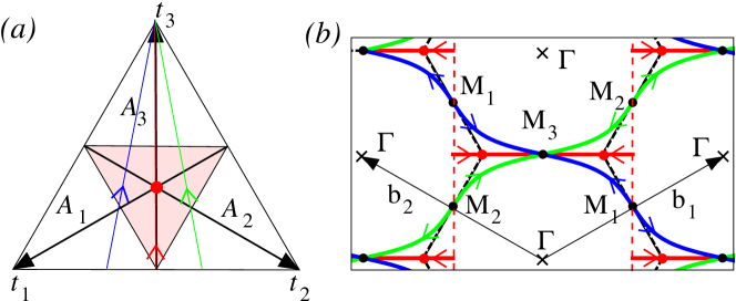
Figure 3: (a) Phase diagram of the asymmetric honeycomb lattice within tight-binding description. Black lines with arrows are coordinate axes for the tunneling amplitudes. Pink central region denotes semimetal with two distinct Dirac points. White regions labeled by $A_{1},A_{2},A_{3}$ denote insulating phases, in which no Dirac points are present. In the insulating phase there is a single band minimum in the first Brillouin zone located at M₁ for $A_{1}$ and so forth. (b) Motion of Dirac points as a function of $t_{3}$ for $t_{1}/t_{2}=1$ (red line in a and b) $t_{1}/t_{2}=3/2$ (blue) $t_{1}/t_{2}=2/3$ (green). Arrows in (a) and (b) indicate direction of motion of Dirac points for increasing $t_{3}$. The symmetric case $t_{1}=t_{2}=t_{3}$ (like in graphene) is indicated by red circles.

We now discuss the eigenspectrum of a honeycomb lattice with asymmetric hoppings, described by the following tight-binding Hamiltonian:

$$H_{\bf k} = -\left(a_{\bf k}^{\dagger},b_{\bf k}^{\dagger}\right)\left(\begin{array}[]{c c}0&\xi_{\bf k}\\ \xi_{\bf k}^{*}&0\end{array}\right)\left(\begin{array}[]{c}a_{\bf k}\\ b_{\bf k}\end{array}\right)\,;\quad\xi_{\bf k}=\sum_{j}t_{j}\exp(-i{\bf k}\cdot{\bf d}_{j})$$ (21)

where $a_{\bf k},b_{\bf k}$ destroy Bloch waves on the two different sublattices and $t_{j}>0$ denote nearest-neighbor hopping energies. For symmetric hoppings the standard Hamiltonian (52) is rediscovered.

A possible realization of this Hamiltonian is a deep optical potential $V({\bf r})$ (3) with different values of $V_{j}$. Due to the inversion symmetry of the confinement potential (3) the onsite energies at the two sublattices are equal and thus can be set to zero in Eq. (21). For asymmetric laser intensities the potentials barriers separating a given potential minimum from the three nearest minima are different. In particular, the corresponding distances between neighboring minima are also different, as follows from Eq. (15). Both effects will lead to asymmetric nearest-neighbor hoppings. We note that a pure shift in the position of the potential minima without a change in the magnitude of the tunnel hopping energies only gives rise to a phase factor in $\xi_{\bf k}$ (21) and thus does not affect the energy spectrum $E_{\bf k}=\pm|\xi_{k}|$.

The energy spectrum of the Hamiltonian (21) is symmetric around zero energy and is given by $E_{\bf k}=\pm|\xi_{k}|$. We note the close analogy between the energy amplitude $\xi_{\bf k}$ and the total electric field $E({\bf r})$. This causes a close similarity between $E_{\bf k}^{2}=|\xi_{\bf k}|^{2}$ and $V({\bf r})\propto E({\bf r})^{2}$. As discussed above for the symmetric case $t_{1}=t_{2}=t_{3}$, valence and conduction band (defined by negative and positive energies, respectively) touch at the two K-points, where they form Dirac cones. Introducing an asymmetry between the tunneling amplitudes the two Dirac points move away from the K-points and approach each other. At a critical asymmetry the Dirac points merge at one of the three inequivalent M-points, and by increasing the asymmetry further a band gap opens.

Figure 3 illustrates the phase diagram and the displacement of the Dirac points as a function of the tunnel amplitudes. The central pink region in Fig. 3a embraces the parameter regime of the semimetallic phase, where the asymmetry is small enough for the two inequivalent Dirac points to exist. It is defined by the condition $|t_{1}-t_{2}|<t_{3}<t_{1}+t_{2}$, which remains invariant under the permutation of the three subindices. The Dirac points are located at ${\bf k}=\pm{\bf k}_{D}$, with:

$${\bf k}_{D}=\left(\begin{array}[]{c}\frac{2}{a}\arccos\left(-\sqrt{\frac{t_{3}^{2}-(t_{2}-t_{1})^{2}}{4t_{1}t_{2}}}\right)\\ \frac{2}{a\sqrt{3}}\;\text{sgn}(t_{1}-t_{2})\arccos\left(\frac{t_{1}+t_{2}}{t_{3}}\sqrt{\frac{t_{3}^{2}-(t_{2}-t_{1})^{2}}{4t_{1}t_{2}}}\right)\end{array}\right)$$ (24)

If necessary the wavevector ${\bf k}_{D}$ as defined above is supposed to be folded back to the first Brillouin zone by adding a uniquely defined reciprocal lattice vector.

Figure 3b shows the displacement of the Dirac points following three different lines of the phase diagram, each defined by a fixed ratio $t_{1}/t_{2}$ while spanned by varying $t_{3}$. We focus first on the red line, which corresponds to the partially symmetric case $t_{1}=t_{2}$ previously studied in Ref. [Zhu et al., 2007]. For $t_{3}=0$ valence and conduction band touch along the extended dashed line. Increasing $t_{3}$ causes the two inequivalent Dirac cones to approach each other along horizontal lines and for symmetric hoppings $t_{1}=t_{2}=t_{3}$ (center of triangle in Fig. 3a) they are located at the K-points. Finally the Dirac cones merge at the symmetry point M${}_{3}=({\bf b}_{1}+{\bf b}_{2})/2$ when $t_{3}=t_{1}+t_{2}$.

In the generic case of $t_{1}\neq t_{2}\neq t_{3}$ one finds the motion shown by the blue and green lines. We now discuss the motion for increasing $t_{3}$. For $t_{3}<|t_{1}-t_{2}|$ the system is an insulator and there is a single band minimum located at M₁, if $t_{1}>t_{2}$ (blue line in region $A_{1}$ of Fig. 3a), or M₂, if $t_{2}>t_{1}$ (green line in region $A_{2}$ of the same figure). While in regions $A_{1}$ or $A_{2}$, the minimum stays pinned at the fixed points M₁ or M₂ and motion along the blue or green line only causes the corresponding gap to decrease until it becomes zero when the central pink triangle is touched (phase transition). For $|t_{1}-t_{2}|<t_{3}<t_{1}+t_{2}$, in both cases (blue and green) the system enters the central triangle of Fig. 3a defining the semimetallic phase, where the band minimum at M₁ or M₂ separates into two Dirac points. The position of the Dirac points are related to each other by the inversion symmetry around the symmetry points $\Gamma$ and M₁, M₂, M₃. Finally at $t_{3}=t_{1}+t_{2}$, where the lines leave the pink triangle in order to enter region $A_{3}$, the Dirac points merge at M₃ and the system undergoes a phase transition from a semimetal to an insulator. Further increase of $t_{3}$ only causes the gap at M₃ to increase.

V Density of states

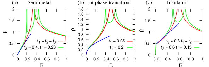
Figure 4: Density of states per unit cell for different hoppings normalized to $t_{1}+t_{2}+t_{3}=1$. (a) Linear energy dependence at low energy within semimetallic phase. (b) Square root energy dependence at phase transition $t_{3}=0.5$. (c) Insulating phase. Blue curves are analytical approximations to red curves given in main text.

We now discuss the density of states, which is defined by $\rho(E)=A^{-1}\sum_{\bf k}\delta(E-E_{\bf k})$, where $A=NA_{u}$ is the area, $N$ the number of unit cells and $A_{u}=a^{2}\sqrt{3}/2$ the size of the unit cell. Characteristic energies are given by the eigenenergies at the symmetry points $E_{\rm M_{3}}=|t_{3}-t_{1}-t_{2}|$, $E_{\rm M_{1}}=|t_{1}-t_{2}-t_{3}|$,$E_{\rm M_{2}}=|t_{2}-t_{1}-t_{3}|$ and $E_{\Gamma}=t_{1}+t_{2}+t_{3}$. $E_{\Gamma}$ is the energy maximum and thus sets the bandwidth. The density has a step at $E=\pm E_{\Gamma}$.

Without loss of generality we focus on the case $t_{3}>t_{1},t_{2}$, so that the energy always has a saddle point at the symmetry points ${\rm M_{2},M_{3}}$, which results in logarithmic van Hove singularities at $E_{\rm M_{2}},E_{\rm M_{3}}$. Whether M₃ is a saddle point or a minimum depends on the tunnel amplitudes. For $t_{3}<t_{1}+t_{2}$ the energy has a saddle point at M₃ and there are two Dirac points in the first Brillouin zone. For symmetric hoppings $t_{3}=t_{1}=t_{2}$ the band structure close to zero energy is given by rotationally symmetric cones centered at the Dirac points. As the hopping energies become different from each other, those cones are stretched and the Dirac points move, but still the density of states vanishes linearly close to zero energy ($E\ll E_{\rm M_{1}},E_{\rm M_{2}}$). In particular for $t_{1}=t_{2}>t_{3}/2$ the low energy spectrum is given by $E_{{\bf k}_{D}+{\bf q}}=\sqrt{v_{x}^{2}q_{x}^{2}+v_{y}^{2}q_{y}^{2}}$, $v_{x}=a\sqrt{4t_{1}^{2}-t_{3}^{2}}/2$, $v_{y}=at_{3}\sqrt{3}/2$, resulting in a density of states $\rho(E)=g_{v}E/2\pi v_{x}v_{y}$, where the degeneracy factor $g_{v}=2$ takes into account the two Dirac points. We note that the velocities $v_{x},v_{y}$ are different if the hoppings are different. While $v_{y}$ increases with increasing $t_{3}$, $v_{x}$ decreases and cancels at the phase transition $t_{3}=2t_{1}=2t_{2}$. Examples of the density of states in the semimetallic phase are given in Fig. 4a.

In the opposite limit $t_{3}>t_{1}+t_{2}$ the energy has its minimum at M₃ and the system is gapped by $2\Delta$ where $\Delta=E_{\rm M_{3}}=t_{3}-t_{1}-t_{2}$. Correspondingly the density of states is zero for $E<\Delta$ and has a finite step at $E=\Delta$. For $t_{1}=t_{2}<t_{3}/2$ the low energy spectrum is given by $E_{{\bf k}_{D}+{\bf q}}=(\Delta^{2}+v_{x}^{2}q_{x}^{2}+v_{y}^{2}q_{y}^{2})^{1/2}$, $v_{x}=a\sqrt{\Delta t_{1}/2}$, $v_{y}=a\sqrt{3t_{1}t_{3}/2}$, leading to a density of states $\rho(E)=\theta(E-\Delta)E/2\pi v_{x}v_{y}$, where $\theta(x)$ denotes the Heaviside step function. This situation is depicted in Fig. 4c.

Right at $t_{3}=t_{1}+t_{2}$ the two Dirac cones merge at M₃ with $E_{\rm M_{3}}=0$, so that M₃ is the minimum of the conduction band, but there is still no band gap. In the particular case $t_{1}=t_{2}=t_{3}/2$, the density of states can be mostly derived analytically:

$$E_{\rm{\bf M}_{3}+{\bf q}} = \frac{t_{3}}{2}\left[6+2\cos(q_{x}a)-8\cos(q_{x}a/2)\cos(\sqrt{3}aq_{y}/2)\right]^{1/2}$$ (25)

$$\rho(E) = \frac{4\sqrt{\epsilon}}{\pi^{2}A_{u}t_{3}}\int_{0}^{1}\frac{dx}{\sqrt{1-x^{2}}\sqrt{1+\epsilon+x^{2}(1-\epsilon)}\sqrt{1-4\epsilon(1-\epsilon)x^{2}}}$$ (26)

with $\epsilon=E/2t_{3}$ denoting the energy in units of the bandwidth. This situation is depicted in Fig. 4b. We note that $E_{\rm{\bf M}_{3}+{\bf q}}\simeq t_{3}[3(aq_{y}/2)^{2}+(a/2)^{4}(q_{x}^{4}-6q_{x}^{2}q_{y}^{2}-3q_{y}^{4})/4]^{1/2}$, which shows that the confinement in the $x$-direction (along which the Dirac points have merged) is much weaker than in the $y$-direction. Equation (26) is valid for the whole energy range $0\leq\epsilon\leq 1$. An expansion around $E=0$ results in:

$$\rho(E) \simeq \frac{4\sqrt{\epsilon}}{A_{u}t_{3}\pi^{2}}\int_{0}^{1}\frac{dx}{\sqrt{1-x^{4}}}=\sqrt{\epsilon}\frac{4\sqrt{\pi}\Gamma(5/4)}{t_{3}A_{u}\pi^{2}\Gamma(3/4)}\simeq\frac{0.53}{A_{u}t_{3}}\sqrt{\frac{E}{2t_{3}}}$$ (27)

Since the square root has a diverging slope at the origin, it can be viewed as a transient behavior between the linear density of states of the semimetallic phase and the step found for the insulating phase. We note that for $\epsilon=0.5$, which is the energy of the two saddle points $E_{\rm M_{1}}=E_{\rm M_{2}}$, the integrand of Eq. (27) contains the factor $(1-x)^{-1}$ which results in a logarithmic divergence in the density of states.

VI Specific heat and structure factor

Finally we discuss two experimental signatures of the phase transition expected when fermions populate the lattice at half filling, namely, the structure factor accessible by Bragg spectroscopyZhu et al. (2007) and the temperature dependence of the specific heatEnsher et al. (1996). The specific heat is defined by $c_{V}\equiv\partial u/\partial T=\frac{\partial}{\partial T}\int\,dE\rho(E)Ef(E)$, where $f(E)$ denotes the Fermi distribution, $u$ the energy density and $\rho(E)$ the density of states as calculated in the previous section. We limit ourselves to the case of half-filling, where the chemical potential $\mu=0$ for all temperatures because of the symmetry of the energy around $E=0$ inherent to the employed tight-binding approximation.

The resulting equations are:

$$u = -\int_{0}^{\infty}\,dE\rho(E)E\tanh(E/k_{B}T)\;;\quad c_{V}=\frac{1}{2k_{B}T^{2}}\int_{0}^{\infty}\,dE\frac{\rho(E)E^{2}}{\cosh^{2}(E/2k_{B}T)}$$ (28)

where we have used $\rho(E)=\rho(-E)$. This results in a different temperature dependence of the specific heat for the different phases:

$$c_{V}\simeq\left\{\begin{array}[]{c c c}T^{2}\,9g_{v}k_{B}^{3}\zeta(3)/2\pi v_{x}v_{y}&;\;\text{for}&\rho(E)=g_{v}E/2\pi v_{x}v_{y}\\[6.45831pt] \left(k_{B}T/t_{3}\right)^{3/2}\,2.1k_{B}/A_{u}&;\;\text{for}&\rho(E)\simeq(E/2t_{3})^{1/2}\,0.53/A_{u}t_{3}\\[6.45831pt] \exp(-\Delta/k_{B}T)\,(6T^{3}+6T^{2}\Delta+3T\Delta^{2}+\Delta^{3})\,2k_{B}^{3}/2\pi v_{x}v_{y}T&;\;\text{for}&\rho(E)\simeq\theta(E-\Delta)E/2\pi v_{x}v_{y}\end{array}\right.$$ (32)

where $\zeta$ denotes the Riemann Zeta Function. Interaction induced corrections to the specific heat in the semimetallic phase have recently been studiedVafek (2007).

As pointed out in Ref. Zhu et al., 2007 another way to experimentally visualize the phase transition is to measure the structure factor by Bragg spectroscopy. We note that the structure factor is up to a constant given by the imaginary part of the dynamical susceptibility which is well known for grapheneGonzález et al. (1994); Wunsch et al. (2006); Hwang and Das Sarma (2007). In fact within the semimetallic phase, the results for the susceptibility of graphene can be easily adapted to include asymmetric hoppings. Noting that $E_{{\bf q}}\simeq\left(v_{x}^{2}q_{x}^{2}+v_{y}^{2}q_{y}^{2}\right)^{1/2}=\kappa$, with $\kappa_{x}=q_{x}v_{x},\kappa_{y}=q_{y}v_{y},\kappa=(\kappa_{x}^{2}+\kappa_{y}^{2})^{1/2}$, one can reuse all formulae of the dynamic susceptibility of arbitrary doping by setting $v_{F}=1$ and replacing $q\to\kappa$.

As an illustration, we state the result for half-filling:

$$S({\bf q},\omega) = \frac{g}{16\pi}\frac{v_{x}^{2}q_{x}^{2}+v_{y}^{2}q_{y}^{2}}{v_{x}v_{y}\sqrt{\omega^{2}-v_{x}^{2}q_{x}^{2}-v_{y}^{2}q_{y}^{2}}}\theta(\omega^{2}-v_{x}^{2}q_{x}^{2}-v_{y}^{2}q_{y}^{2})$$ (33)

Here $g=2$ is due to the two Dirac points (valley degeneracy). For $t_{1}=t_{2}>t_{3}/2$ the velocities are given by $v_{x}=a\left(4t_{1}^{2}-t_{3}^{2}\right)^{1/2}/2$, $v_{y}=at_{3}\sqrt{3}/2$. We note that in Ref. Zhu et al., 2007 only the energy spectrum was considered while the overlap factor $f^{\lambda^{\prime}\lambda}({\bf k},{\bf q})$ resulting from the spinor eigenfunctions was ignored. Therefore the $\omega^{2}$ term present in the numerator of Eq. (8) of Ref. Zhu et al., 2007 is absent in Eq. (33) above. We note that $f^{\lambda^{\prime}\lambda}({\bf k},{\bf q})=|u_{{\bf k}+{\bf q},\lambda^{\prime}}^{*}u_{{\bf k}\lambda}|^{2}$ describes how easily the spinor wavefunction $u_{{\bf k}\lambda}$ ($\lambda=\mp 1$ labels valence and conduction band) can be scattered in to $u_{{\bf k}+{\bf q},\lambda^{\prime}}$ and is responsible for example for the absence of backscattering and the Klein paradox in graphene.Katsnelson et al. (2006) The general form of the spinor wavefunction for the tight-binding Hamiltonian (21), is $u_{{\bf k}\,\lambda}=2^{-1/2}(-\lambda\,\xi_{\bf k}/|\xi_{\bf k}|,1)$.

For the gaped case $t_{1}=t_{2}<t_{3}/2$, an analytical formula for the structure factor at half-filling and for energies close to the gap $E_{\bf q}\approx\left(\Delta^{2}+v_{x}^{2}q_{x}^{2}+v_{y}^{2}q_{y}^{2}\right)^{1/2}\simeq\Delta+\frac{v_{x}^{2}}{2\Delta}q_{x}^{2}+\frac{v_{y}^{2}}{2\Delta}q_{y}^{2}$ is given by:

$$S({\bf q},\omega) = \theta(\omega-2\Delta-\frac{v_{x}^{2}q_{x}^{2}}{4\Delta}-\frac{v_{y}^{2}q_{y}^{2}}{4\Delta})\frac{3a^{2}q_{y}^{2}}{4(t_{3}/t_{1}-2)^{2}}\frac{\Delta}{2\pi v_{x}v_{y}}$$ (34)

While the step function originates from the single particle eigenspectrum, the whole ${\bf q}$-dependence arises from the spinor character of the wavefunctions captured in the factor $f^{\lambda^{\prime}\lambda}({\bf k},{\bf q})$ described above.

VII Topological properties

Interestingly, a gap only opens after the two Dirac points have merged. Mathematically it is straightforward to show that an energy minimum of the conduction band that is not located at one of the symmetry points M₁, M₂, M₃, $\Gamma$ is automatically a Dirac point. To show this, we note that a minimum of the conduction band is a root of $\nabla_{\bf k}E_{\bf k}^{2}=\nabla_{\bf k}\left(\eta_{\bf k}\eta_{\bf k}^{*}\right)$, with $\eta_{\bf k}=t_{3}+t_{1}\exp(i{\bf k}{\bf a}_{1})+t_{2}\exp(i{\bf k}{\bf a}_{2})$.

$$\nabla_{\bf k}\left(\eta_{\bf k}\eta_{\bf k}^{*}\right) = {\bf v}_{1}{\rm Re}(\eta_{\bf k})+{\bf v}_{2}{\rm Im}(\eta_{\bf k})$$ (35)

$${\bf v}_{1} = 2\nabla_{\bf k}{\rm Re}(\eta_{\bf k})=-2\left[t_{1}\sin({\bf a}_{1}\cdot{\bf k}){\bf a}_{1}+t_{2}\sin({\bf a}_{2}\cdot{\bf k}){\bf a}_{2}\right]$$

$${\bf v}_{2} = 2\nabla_{\bf k}{\rm Im}(\eta_{\bf k})=2\left[t_{1}\cos({\bf a}_{1}\cdot{\bf k}){\bf a}_{1}+t_{2}\cos({\bf a}_{2}\cdot{\bf k}){\bf a}_{2}\right]$$

Since ${\bf a}_{1},{\bf a}_{2}$ are linear independent, ${\bf v}_{1},{\bf v}_{2}$ are also linear independent, unless $\sin\left(({\bf a}_{2}-{\bf a}_{1})\cdot{\bf k})\right)=0$, a condition is only fulfilled at the symmetry points M₁,M₂,M₃,$\Gamma$. This analysis shows that a minimum which is not located at a symmetry point, is necessarily a Dirac point, since then both the imaginary and the real parts of $\eta_{\bf k}$ vanish and therefore the energies are $E_{\mp,{\bf k}}=\mp|\eta_{\bf k}|=0$. Furthermore, these minima always occur in pairs due to time reversal symmetry (inversion symmetry around the $\Gamma$-point).

The deeper reason for the stability of the Dirac points is the momentum space topology of the Bloch wavefunctionsMañes et al. (2007); Bergman et al. (2008). This is nicely illustrated by noting that the Berry phase, defined asBerry (1984) $\phi_{B}=i\oint_{S}d{\bf k}\langle u_{\bf k}|\nabla_{\bf k}|u_{\bf k}\rangle$ with $S$ denoting a closed path in reciprocal space, takes values $\pm\pi,0$ depending on whether $S$ encloses one Dirac point, or the other, or both. Thus each Dirac point is a source of a $\pm\pi$ delta-function flux of Berry curvature, and this flux remains invariant under perturbations that preserve space and time inversion symmetryMañes et al. (2007); Bergman et al. (2008). Only if the two Dirac points merge the Berry curvature vanishes within the whole first Brillouin zone and a gap can open.

We note that the Dirac points are unstable against perturbations that break spatial invariance. Examples are substrate-induced gap opening in graphene due to breaking of sublattice symmetryZhou et al. (2007) or honeycomb lattices where nearest-neighbor hoppings are periodically modified to form a Kekulé patternHou et al. (2007).

VIII Summary and conclusions

We have studied the electronic structure and the phase diagram of non-interacting fermions confined to hexagonal optical lattices. In the first part of the paper, we have analyzed the appearance of Dirac points in the band structure of fermionic atoms populating triangular and honeycomb optical lattices for different confinement strengths. Numerical results were complemented by analytical equations both for strong and weak potentials. The Dirac points arising in honeycomb and triangular lattices differ in several important aspects. While in honeycomb lattice the Dirac cone is isolated, it resonates with a continuum band for a triangular lattice. Furthermore, in honeycomb lattices the Fermi-energy coincides with the Dirac point for integer filling, while a non-integer filling is needed in the case of a triangular lattice. For the honeycomb lattice the first pair of Dirac points arises from the touching of the two lowest bands, which within a tight-binding description stem from the ground state of the two potential minima per unit cell. By contrast, for a triangular lattice the first pair of Dirac points occurs at the touching of the second and third band, which within a tight-binding description are formed by the doubly degenerate first excited state of the single potential minimum per unit cell.

In the second part of this work, we have focused on the phase diagram and the evolution of the Dirac points in honeycomb lattices adopting a tight-binding description with asymmetric nearest-neighbor hoppings. The semimetallic phase is not only realized for strictly symmetric hoppings but rather for an extended region of the hopping parameter space. This stability of the semimetallic phase is based on topology. With increasing asymmetry the Dirac points approach each other along continuous trajectories and at a critical asymmetry they finally merge and an energy gap opens. We derive analytic formulae for the trajectories of the Dirac points as well as for the density of states. Right at the phase transition the density of states increases like $\sqrt{E}$, which interpolates between the linear dependence of the semimetallic phase and the step-like increase of the insulating phase. We also show how the phase transition becomes manifest in a change of the temperature dependence of the specific heat as well as in the properties of the structure factor.

An interesting follow-up of this work concerns the influence of interactions on the phase diagram, since optical lattices permit a systematic control of the effective interaction strength by using Feshbach resonances or modifying the lattice propertiesBloch et al. (2008).

Appendix A Dirac cones in weak symmetric lattices

Here we apply the nearly-free-particle approximation to derive the eigenspectrum determined by Eq. (16) with $V_{1}=V_{2}=V_{3}=V$ close to the K-point. In absence of any potential the dispersion relation at the K-point is three-fold degenerate, where the three states can be labeled by the ${\bf k}$-values ${\bf k}\in\{{\bf K},{\bf K}-{\bf G}_{10},{\bf K}-{\bf G}_{11}\}$. Treating the lattice within lowest order perturbation theory, the eigenvalue problem at ${\bf k}={\bf K}+{\bf q}$ has then the following form:

$$\left(\begin{array}[]{c c c}E^{0}_{{\bf K}+{\bf q}}&V/2&V/2\\ V/2&E^{0}_{{\bf K}-{\bf G}_{10}+{\bf q}}&V/2\\ V/2&V/2&E^{0}_{{\bf K}-{\bf G}_{11}+{\bf q}}\end{array}\right)\left(\begin{array}[]{c}c_{{\bf K}+{\bf q}}\\ c_{{\bf K}-{\bf G}_{10}+{\bf q}}\\ c_{{\bf K}-{\bf G}_{11}+{\bf q}}\end{array}\right)=E_{{\bf K}+{\bf q}}\left(\begin{array}[]{c}c_{{\bf K}+{\bf q}}\\ c_{{\bf K}-{\bf G}_{10}+{\bf q}}\\ c_{{\bf K}-{\bf G}_{11}+{\bf q}}\end{array}\right)$$ (45)

The solutions of the above eigenproblem for ${\bf q}=0$ are given by $E=E^{0}_{\bf K}+V$ with eigenvector $3^{-1/2}(1,1,1)$ and $E=E^{0}_{\bf K}-V/2$, which is two fold degenerate with a possible set of orthonormal eigenvectors given by: ${\bf v}_{1}=2^{-1/2}(-1,1,0)$ and ${\bf v}_{2}=6^{-1/2}(-1,-1,2)$. We note that the remaining two-fold degeneracy is protected by topology and thus persists beyond a perturbative description. This degeneracy occurs in the ground state for $V>0$ (honeycomb lattice) and in the first excited state for $V<0$ (triangular lattice).

The remaining two-fold degenaracy of ${\bf v}_{1},{\bf v}_{2}$ disappears for finite ${\bf q}$. The effective two-band Hamiltonian spanned by ${\bf v}_{1}$,${\bf v}_{2}$ is given by:

$$\left(H_{\rm eff}({\bf q})\right)_{ij} = \langle v_{i}|H({\bf q})|v_{j}\rangle$$ (46)

$$H_{\rm eff}({\bf q}) = \left(E^{0}_{\bf K}-V/2+E^{0}_{\bf q}\right)\mathbbm{1}+\hbar v_{F}\left(-\frac{q_{x}}{2}+\frac{\sqrt{3}}{2}q_{y}\right)\sigma_{z}+\hbar v_{F}\left(\frac{\sqrt{3}}{2}q_{x}+\frac{1}{2}q_{y}\right)\sigma_{x}$$ (47)

with $v_{F}=2\pi\hbar/3am$. The eigenenergies are given by $E_{{\bf K}+{\bf q}}=E^{0}\pm\hbar v_{F}q$ with $E_{0}=E^{0}_{{\bf K}}-V/2+E^{0}_{\bf q}$. We note that the effective Hamiltonian can be transformed by a unitary transformation to $\tilde{H}_{\rm eff}=E_{0}\mathbbm{1}+\hbar v_{F}(q_{x}\sigma_{x}+q_{y}\sigma_{y})$, which is identical (except for the value of $v_{F}$) to the low-energy Hamiltonian obtained in the tight-binding approximation .

Appendix B Tight-binding description for symmetric potentials

B.1 Symmetric honeycomb lattice

For the honeycomb lattice there are two degenerate minima per unit cell and for sufficiently deep potential wells [i.e. for $V\ll\frac{\hbar^{2}}{2ma^{2}}$, with $m$ the atomic mass and $V$ the confinement amplitudes of Eq. (3)] the basis for the two lowest bands can be restricted to the ground state of each minimum. In the symmetric case (equal laser intensities) the potential around each minimum is rotationally symmetric and harmonic and the minima form a honeycomb lattice. Thus the nearest-neighbor hoppings $t$ are all the same.

$$H = -t\sum_{i}a^{\dagger}({\bf r}_{i})\sum_{j}b({\bf r}_{i}+{\bf d}_{j})+{\rm H.c.}=-\sum_{\bf k}\left(a_{\bf k}^{\dagger},b_{\bf k}^{\dagger}\right)\left(\begin{array}[]{c c}0&\xi_{\bf k}\\ \xi_{\bf k}^{*}&0\end{array}\right)\left(\begin{array}[]{c}a_{\bf k}\\ b_{\bf k}\end{array}\right)\,;\quad\xi_{\bf k}=t\sum_{j}\exp(-i{\bf k}\cdot{\bf d}_{j})$$ (52)

Here $a({\bf r})$ destroys a particle at the A-site at position ${\bf r}$ and the ${\bf d}_{j}$ denotes the vectors connecting an A-site with its neighboring B-sites, see Fig. 1b. Fourier transformation is given by $a({\bf r}_{i})=N^{-1/2}\sum_{\bf k}\exp(i{\bf k}\cdot{\bf r}_{i})a_{\bf k}$, where $N$ is the number of unit cells. The eigenenergies of the above Hamiltonian are given by: $E_{\bf k}=\pm|\xi_{k}|=\pm t[3+2\cos(k_{y}a)+4\cos(\sqrt{3}ak_{x}/2)\cos(ak_{y}/2)]^{1/2}$. The energy spectrum is symmetric around $E=0$, where the Fermi surface only consists of singular (Dirac) points located at the K-points. Close to the K-point one can approximate $\xi_{{\bf K}+{\bf q}}\simeq-v_{F}(q_{x}-iq_{y})$ with $v_{F}=\sqrt{3}at/2$, so that the Hamiltonian close to the K-point can be written as $H_{\rm eff}=\hbar v_{F}(q_{x}\sigma_{x}+q_{y}\sigma_{y})$ with eigenenergies $E_{\bf q}=\pm\hbar v_{F}q$.

B.2 Symmetric triangular lattice

The triangular lattice has one minimum per unit cell. For a symmetric lattice the potential around the minimum is rotationally symmetric and harmonic. The ground state of such a minimum is non-degenerate while the first excited state is two fold degenerate and can be represented by $p_{x}(x,y)=\psi_{1}(x)\psi_{0}(y)$ and $p_{y}(x,y)=\psi_{0}(x)\psi_{1}(y)$, where $x,y$ are measured with respect of the center of the minimum and $\psi_{0}(x),\psi_{1}(x)$ denote the ground state and the first excited state of the one-dimensional harmonic oscillator.

Figure 5: (a) Triangular lattice with schematic representation of the two degenerate excited $\pi$ orbitals. (b) Top $t_{\sigma}$, bottom $t_{\pi}$.

The band arising from the ground state is described by the following tight-binding Hamiltonian:

$$H = -t\sum_{\langle i,j\rangle}c^{\dagger}_{i}c_{j}=\sum_{{\bf k}}E_{\bf k}c_{\bf k}^{\dagger}c_{\bf k}\,;\quad E_{\bf k}=-2t\left[\cos({\bf k}\cdot{\bf a}_{1})+\cos({\bf k}\cdot{\bf a}_{2})+\cos({\bf k}\cdot({\bf a}_{1}-{\bf a}_{2}))\right]$$ (53)

The hopping between the $p_{x}$ and $p_{y}$ orbitals is no longer isotropicWu et al. (2007). As visualized in Fig. 5b, we introduce the hopping amplitudes $t_{\sigma}$ and $t_{\pi}$ depending on the relative orientation of the orbitals. Non-parallel hoppings (e.g. from $p_{x}$ to $p_{y}$) are excluded by the symmetry of the wavefunctions.

The tight-binding Hamiltonian describing the two bands arising from the two-fold degenerate first excited state is then given by:

$$H = \sum_{{\bf k}}\left(c_{\bf k}^{\dagger},d_{\bf k}^{\dagger}\right)H_{k}\left(\begin{array}[]{c}c_{\bf k}\\ d_{\bf k}\end{array}\right)\,;\quad H_{\bf k}=h_{1}\mathbbm{1}+h_{2}\sigma_{x}+h_{3}\sigma_{z}\,;\quad E_{\bf k}=h_{1}\pm\sqrt{h_{2}^{2}+h_{3}^{2}}$$ (56)

$$\left(\begin{array}[]{c}t_{c}\\ t_{r}\end{array}\right) = \left(\begin{array}[]{c c}1/2&1/2\\ -1&1\end{array}\right)\left(\begin{array}[]{c}t_{\sigma}\\ t_{\pi}\end{array}\right)\;;\quad h_{1}=2t_{c}\left[\cos(ak_{x})+2\cos(ak_{x}/2)\cos(ak_{y}\sqrt{3}/2)\right]$$ (63)

$$h_{2} = \sqrt{3}t_{r}\sin(ak_{x}/2)\sin(ak_{y}\sqrt{3}/2)\;;\quad h_{3}=t_{r}\left[\cos(ak_{x}/2)\cos(ak_{y}\sqrt{3}/2)-\cos(ak_{x})\right]$$

We note that both bands touch at the $\Gamma$ point as well as at the K-points (see Figs 1c and 2). The energies are given by $E_{\Gamma}=6t_{c}$ and $E_{\bf K}=-3t_{c}$, while at the M-point the energies are split with $E_{\rm M}=-2t_{c}\pm 2t_{r}$. Around the K-points ${\bf k}={\bf K}+{\bf q}$ the energy dispersion to linear order in ${\bf q}$ is rotationally symmetric, $E_{{\bf K}+{\bf q}}=-3t_{c}\pm 3^{3/2}at_{r}q/4+{\cal O}({\bf q}^{2})$, so that a circular Dirac cone is formed around each K-point. We note that the electronic structure of a triangular lattice with degenerate $d$-orbitals shows similar featuresGuillamon et al. (2008).

References

- Novoselov et al. (2004) K. S. Novoselov, A. K. Geim, S. V. Morozov, D. Jiang, Y. Zhang, S. V. Dubonos, I. V. Grigorieva, and A. A. Firsov, Science 306, 666 (2004).
- Castro Neto et al. (2007) A. H. Castro Neto, F. Guinea, N. M. R. Peres, K. S. Novoselov, and A. K. Geim (2007), eprint arXiv:0709.1163.
- Geim and Novoselov (2007) A. K. Geim and K. S. Novoselov, Nature Materials 6, 183 (2007).
- Beenakker (2007) C. Beenakker (2007), eprint arXiv:0710.3848.
- Zhang et al. (2005) Y. B. Zhang, Y. W. Tan, H. L. Stormer, and P. Kim, Nature 438, 201 (2005).
- Novoselov et al. (2005) K. S. Novoselov, A. K. Geim, S. V. Morozov, D. Jiang, M. I. Katsnelson, I. V. Grigorieva, S. V. Dubonos, and A. A. Firsov, Nature 438, 197 (2005).
- Grynberg et al. (1993) G. Grynberg, B. Lounis, P. Verkerk, J.-Y. Courtois, and C. Salomon, Phys. Rev. Lett. 70, 2249 (1993).
- Zhu et al. (2007) S.-L. Zhu, B. Wang, and L.-M. Duan, Phys. Rev. Lett. 98, 150404 (2007).
- Hou et al. (2007) C.-Y. Hou, C. Chamon, and C. Mudry, Phys. Rev. Lett. 98, 186809 (2007).
- Herbut (2007) I. F. Herbut, Phys. Rev. Lett. 99, 206404 (2007).
- Zhang et al. (2008) W. Zhang, P. Zhang, S. Duan, and X.-G. Zhao (2008), eprint arXiv:0805.2736.
- Dudarev et al. (2004) A. M. Dudarev, R. B. Diener, I. Carusotto, and Q. Niu, Phys. Rev. Lett. 92, 153005 (2004).
- Wu and Das Sarma (2007) C. Wu and S. Das Sarma (2007), eprint arXiv:0712.4284.
- Wu et al. (2007) C. Wu, D. Bergman, L. Balents, and S. Das Sarma, Phys. Rev. Lett. 99, 070401 (2007).
- Wu (2008) C. Wu (2008), eprint arXiv:0805.3525.
- Shao et al. (2008) L. B. Shao, S.-L. Zhu, L. Sheng, D. Y. Xing, and Z. D. Wang (2008), eprint arXiv:0804.1850.
- Haldane (1988) F. Haldane, Phys. Rev. Lett. 61, 2015 (1988).
- Haldane and Raghu (2008) F. D. M. Haldane and S. Raghu, Phys. Rev. Lett. 100, 013904 (2008).
- Raghu and Haldane (2006) S. Raghu and F. D. M. Haldane (2006), eprint arXiv:cond-mat/0602501.
- Sepkhanov et al. (2008) R. A. Sepkhanov, J. Nilsson, and C. W. J. Beenakker (2008), eprint arXiv:0803.1581.
- Mañes et al. (2007) J. Mañes, F. Guinea, and A. H. Vozmediano, Phys. Rev. B. 75, 155424 (2007).
- Ensher et al. (1996) J. R. Ensher, D. S. Jin, M. R. Matthews, C. E. Wieman, and E. A. Cornell, Phys. Rev. Lett. 77, 4984 (1996).
- Vafek (2007) O. Vafek, Phys. Rev. Lett. 98, 216401 (2007).
- González et al. (1994) J. González, F. Guinea, and V. A. M. Vozmediano, Nucl. Phys. B 424, 595 (1994).
- Wunsch et al. (2006) B. Wunsch, T. Stauber, F. Sols, and F. Guinea, New J. Phys. 8, 318 (2006).
- Hwang and Das Sarma (2007) E. H. Hwang and S. Das Sarma, Phys. Rev. B. 75, 205418 (2007).
- Katsnelson et al. (2006) M. I. Katsnelson, K. S. Novoselov, and A. K. Geim, Nature Phys. 2, 620 (2006).
- Bergman et al. (2008) D. L. Bergman, C. Wu, and L. Balents (2008), eprint arXiv:0803.3628.
- Berry (1984) M. V. Berry, Proc. R. Soc. Lond. A 392, 45 (1984).
- Zhou et al. (2007) S. Zhou, G.-H. Gweon, A. Fedorov, P. First, W. de Heer, D.-H. Lee, F. Guinea, A. C. Neto, and A. Lanzara, Nature Materials 6, 770 (2007).
- Bloch et al. (2008) I. Bloch, J. Dalibard, and W. Zwerger, Rev. Mod. Phys. 80, 885 (2008).
- Guillamon et al. (2008) I. Guillamon, H. Suderow, F. Guinea, and S. Viera, Phys. Rev. B. 77, 134505 (2008).