Combinatorial cell complexes and Poincare duality

Abstract.

We define and study a class of finite topological spaces, which model the cell structure of a space obtained by gluing finitely many Euclidean convex polyhedral cells along congruent faces. We call these finite topological spaces, combinatorial cell complexes (or c.c.c). We define orientability, homology and cohomology of c.c.c’s and develop enough algebraic topology in this setting to prove the Poincare duality theorem for a c.c.c satisfying suitable regularity conditions. The definitions and proofs are completely finitary and combinatorial in nature.

1. Introduction

1.1.

Summary of results: Given a topological space with a triangulation, if we only remember the set of simplices and incidence relations among them, we get a simplicial complex. One can think of the partially ordered set of the simplicial complex as a finite topological space and study how the combinatorics of this poset reflects the algebraic topology of the space one started with. In this article we want to do something similar, but we want to allow our cells to have more general shapes, not just of simplices. (For example, cells in the shape of any convex polyhedron are allowed). We shall call these objects combinatorial cell complex or c.c.c for short. Let $X$ be a topological space written as a finite union of a collection $S_{X}$ of Euclidean convex polyhedra. Assume that $S_{X}$ is closed under intersection and that the intersection of two distinct polyhedron in $S_{X}$ of equal dimension, has strictly lower dimension. If we forget the space $X$ and only remember the set $S_{X}$, the dimension of each polyhedron and the partial order coming from incidence relation among the elements of $S_{X}$, we get an example of a c.c.c.

Thus, a c.c.c $S$ is a partially ordered set, with a rank (or dimension) function defined on $S$, satisfying some axioms (the definition is given in 2.2). The elements of $S$ are called cells. The axioms describe how the cells are allowed to be glued together; they try to mimic the conditions that are satisfied if $S$ was obtained from polyhedral decomposition of a space $X$, as above. Our objective here are the following:
(A) We want to see how to translate into $S_{X}$, the topological properties of $X$, via the correspondence $X\to S_{X}$. For example, we shall call $S$ manifold–like, if it satisfies some extra conditions that would obviously hold, if $S=S_{X}$ for some manifold $X$. The key definition is that of an orientable c.c.c (see 4.1).
(B) Once we have put enough regularity conditions on a c.c.c to remove the pathologies, we want to see how much algebraic topology can be developed in this combinatorial setting. In particular, we define cellular homology and cohomology groups of c.c.c’s with orientable cells and prove a Poincare duality theorem stated below (see theorem 9.2).

Theorem. Let $S$ be an orientable, manifold–like c.c.c of dimension $n$. Suppose each cell of the c.c.c $S$ and the opposite c.c.c $S^{\circ}$ is flag–connected and acyclic. Then $H_{i}(S)\simeq H^{n-i}(S)$.

(The definitions of the various terms are given in the following sections: flag–connected and orientable: 4.1, manifold–like: 3.1, $S^{\circ}$: 3.3, acyclic: 7.1. Homology and cohomology groups are defined in section 5). If $S=S_{X}$ for some space $X$, then these homology groups are the same as the cellular homology groups of $X$. In particular, a simplicial complex gives a c.c.c and in this situation, our homology groups are identical with simplicial homology groups (see 5.7).

The main technical part in the proof of theorem 9.2 is to show that, under the conditions of the theorem, the homology of $S$ is invariant under “barycentric subdivision” (see proposition 8.5). It follows (see 10.2), that under these regularity conditions, the homology groups of the c.c.c $S$ coincide with the homology groups of the simplicial set $N(S)$ obtained by taking the nerve of the poset $S$ (or, in other words, the singular homology of the topological space obtained by taking geometric realization of $N(S)$). Sections 6, 7 and 8 are mainly occupied with proving 8.5. Given the technical result 8.5, the proof of the theorem 9.2 is totally transparent. This argument, given in section 9, can be read right after we are through with the definitions in section 5.

1.2.

Relationship with simplicial topology: The standard approach for translating algebraic topology in a combinatorial setting is via simplicial sets (e.g. see [9]), which are abstract versions of simplicial complexes with labeling of vertices. Our main reason for introducing a combinatorial setting with more general cell shapes is the following:

In the classical proof of Poincare duality, one relates homology and cohomology by taking the dual of a cell complex (e.g. see [7]). However, the cells of the dual cell complex of a simplicial complex need not be simplices. We allow more general cell shapes so that the duality is built into the setup (the dual of a c.c.c $S$ has the same underlying set as $S$, with the partial order and rank reversed).

One disadvantage of the present setup is the lack of explicit functoriality of homology groups. In general, given a continuous map (that is, an order preserving function) $f\colon\thinspace S\to S^{\prime}$ between c.c.c’s, there is no obvious chain map from the chain complex of $S$ (as defined in section 5) to that of $S^{\prime}$, inducing a map between the cellular homology groups. However, if $S$ and $S^{\prime}$ satisfy the regularity conditions given in the Poincare duality theorem above, then one does get a map $H_{i}(f)\colon\thinspace H_{i}(S)\to H_{i}(S^{\prime})$, so that $H_{i}$ becomes a functor. Unfortunately, we are only able to see this by using the invariance of homology under barycentric subdivision (see 8.5, 8.6), and the consequent canonical isomorphism between the homology of a c.c.c $S$ (with enough regularity conditions) and that of the simplicial set $N(S)$ (see 10.2). The functoriality of the cellular homology groups follows by invoking the functoriality of homology of simplicial sets.

As was suggested by Peter May (private communications), it would be nice to have a shape category so that (some variant of) a c.c.c becomes a presheaf (of sets) on this shape category. Then one could develop the theory as for simplicial sets in a functorial way. This possibility also makes us wonder if the combinatorial study of shapes of cells might have some bearings on certain approaches to higher category theory, notably those initiated by Steet in [13] and by Baez–Dolan in [2]. In these approaches, much of the structure of the higher category is encoded in the shape of the cells that represent the higher morphisms. For an introduction to these ideas, see chapter 6 and 4 in [4].

1.3.

Finite topological spaces: The topology of finite spaces can be surprisingly rich. For example, there are finite spaces having weak homotopy type of any finite simplicial complex (see [12]). The finite topological spaces have been studied since they were introduced by Alexandroff in [1] and the theory of simple homotopy types was developed by Whitehead in [15]. The simple homotopy types of polyhedra were studied using finite topological spaces in the recent article [3]. We refer the reader to the notes [10] and [11] for an introduction to the topology of finite spaces and to [14] for a survey of the combinatorial aspects of this theory. The book [8] is a convenient reference for combinatorial algebraic topology.

In this article we have restricted our study to purely combinatorial aspects of the theory of c.c.c’s. The close relationship between the topology of a cell complex and that of the corresponding finite space has not been explored or utilized here. This, and other topological questions, like the relationship between the homology of a c.c.c $S$ defined here and the singular homology of the finite space $S$, will hopefully be explored in a later article.

1.4.

Organization of the paper: The arguments in this article are, in most places, logically self contained. The proof of some technical lemmas have been relegated to an appendix to arrive at the main theorem 9.2 quickly. An index of some frequently used symbols is included below.

Acknowledgments: I would like to thank Prof. Gabriel Minian for many useful comments on reading an early draft of this article. I would like to thank Prof. Richard Borcherds and Prof. Jon Alperin for suggesting useful references. Most of all, I would like to thank Prof. Peter May for his encouragement and many interesting and illuminating discussions since the early stages of this work.

1.5.

Index of some commonly used notation: Let $S$ be a c.c.c. Let $T$ be a subset of $S$ and $x$, $y$ be elements of $S$.

$C_{i}(S)$	the set of $i$–chains in the c.c.c $S$, that is, the free abelian group on the $i$–cells of $S$.
$C_{x}(y)$	a “new cell” in the stellar subdivision $S^{x}$, called the cone on $y$ with vertex at $x$.
$\operatorname{cl}(x)$	the set of cells less than or equal to $x$, that is, the closure of $x$.
$\Delta(x)$	the set of faces of $x$.
$\partial$	the boundary map on chain complexes.
$\mathcal{F}(S)$	the set of flags in $S$. (We write $\mathcal{F}(x)=\mathcal{F}(\operatorname{cl}(x))$).
$\gamma$	usually a flag (except in lemma 5.7, where it is a simplex).
$M(x)$	$=\operatorname{star}(x)\setminus U(x)$.
$\nabla(x)$	the set of co-faces of $x$.
$\omega$	an orientation. ($\omega_{x}$ denotes an orientation on $\operatorname{cl}(x)$).
$\operatorname{rk}(x)$	the rank of a cell $x$.
$S$	usually a combinatorial cell complex (called c.c.c for short).
$S^{\circ}$	the opposite c.c.c of $S$.
$S(r)$	the set of cells of $S$ having rank $r$.
$S^{(1)}$	the first barycentric subdivision of $S$.
$S^{x}$	the stellar refinement of $S$ at $x$. We shall write $(S^{x})^{y}=S^{xy}$.
$s(x,y)$	a sign assigned to each pair $\{x,y\}$, where $x$ is a cell and $y$ is a face of $x$, with
	orientations given on $\operatorname{cl}(x)$ and $\operatorname{cl}(y)$ (see 4.4).
$\operatorname{star}(x)$	$=\operatorname{cl}(U(x))$, that is, the set of cells $y$ such that $x$ and $y$ have an upper bound.
$U(x)$	the set of cells greater than or equal to $x$.
$\vee T$	the least upper bound of $T$; we write $x\vee y=\vee\{x,y\}$.
$\wedge T$	the greatest lower bound of $T$; we write $x\wedge y=\wedge\{x,y\}$.
$X$	usually a combinatorial cell complex (called c.c.c for short).
$x,y,z$	usually any of these letters denote a cell of a c.c.c.

2. basic definitions

2.1.

The setup: Suppose we are given a finite partially ordered set $(S,\leq)$ and a function, denoted by $\operatorname{rk}$, from $S$ to non-negative integers such that $y<x$ implies $\operatorname{rk}(y)<\operatorname{rk}(x)$. Given this data, we introduce the following notation and nomenclature:

If there is a possibility of confusion, we shall write $\leq_{S}$ to denote the partial order on $S$. Elements of $S$ are called cells. If $\operatorname{rk}(x)=r$, we say that $x$ is a cell of rank $r$ or $x$ is an $r$–cell. Write $S$ as a disjoint union, $S=\cup_{r=0}^{\infty}S(r)$, where $S(r)$ is the set of $r$–cells of $S$. If $x>y,$ we say that $x$ is above $y$ or that $y$ is below $x$. More precisely, we say that $y$ is a facet of $x$ of co-dimension $(\operatorname{rk}(x)-\operatorname{rk}(y))$. A co-dimension one facet of $x$ is called a face of $x$. The set of faces of $x$ is denoted by $\Delta_{S}x$ or $\Delta x$, if there is no possibility of confusion. Dually, the cells that have $x$ as one of their face are called the co-faces of $x$. The set of co-faces of $x$ is denoted by $\nabla x$. The set of cells greater than or equal to $x$ (resp. less than or equal to $x$) is denoted by $U_{S}(x)=U(x)$ (resp. $\operatorname{cl}_{S}(x)=\operatorname{cl}(x)$).

Let $T$ be a subset of $S$. An element $x\in S$ is an upper bound of $T$, if $x\geq z$ for all $z\in T$. The least upper bound of $T$, denoted by $\vee T$, is an upper bound of $T$ such that $\vee T\leq y$, for every upper bound $y$ of $T$. Similarly, one defines the greatest lower bound of $T$, denoted by $\wedge T$. Of course least upper bound or greatest lower bound of $T$ may not exist. One also writes $x\vee y$ to denote $\vee\{x,y\}$ and $x\wedge y$ to denote $\wedge\{x,y\}$. If $z=x\wedge y$, we say that $x$ and $y$ meet at $z$. For $T\subseteq S$, let $\Delta T=\cup_{x\in T}\Delta x$. Inductively define $\Delta^{j}T=\Delta(\Delta^{j-1}T)$. The rank zero cells below $x$ are called the vertices of $x$.

2.2 Definition.

We say that $S$ is a combinatorial cell complex or c.c.c for short, if the data $(S,\leq,\operatorname{rk})$ satisfies the following four axioms:

1. The partial order is compatible with rank, that is, if $y<x$, then $\operatorname{rk}(y)<\operatorname{rk}(x)$.

2. The collection $S$ has enough cells, in the following sense. If $T$ is a subset of $S$ that is bounded below, then the greatest lower bound $\wedge T$ exists. For all $x$ and $y$ in $S$ with $y<x$, there exists a cell $y^{\prime}$ such that $\operatorname{rk}(y^{\prime})=\operatorname{rk}(y)+1$ and $y<y^{\prime}\leq x$.

3. Each cell $x\in S$ of rank at-least one is the least upper bound of its faces, that is, $x=\vee\Delta x$.

4. If $y$ is a co-dimension $2$ facet of $x$, then there are exactly two faces of $x$ that are above $y$ and these two cells meet at $y$. In other words, given $y\in S(i-1)$, $x\in S(i+1)$, $y<x$, there exists distinct cells $y_{+}$ and $y_{-}$ in $S(i)$ such that $\Delta x\cap\nabla y=\{y_{+},y_{-}\}$.

2.3 Example.

Let $T$ be an finite abstract simplicial complex (see definition 2.1 in [8]). The set $T$ becomes a combinatorial cell complex with the partial order given by set inclusion. A simplex with $(r+1)$ vertices has rank $r$. Given a collection of simplices $T_{1}\subseteq T$, that is bounded below, the greatest lower bound of $T_{1}$ is $\wedge T_{1}=\cap_{\sigma\in T}\sigma$. A co-dimension 2 facet of a simplex $\sigma$ has the form $\sigma\setminus\{x_{i},x_{j}\}$, where $x_{i}\neq x_{j}$ are two vertices of $\sigma$. The two simplices in between, are $\sigma\setminus\{x_{i}\}$ and $\sigma\setminus\{x_{j}\}$.

A topological space with a polyhedral decomposition defines a combinatorial cell complex. Note that an $r$–cell has at-least $(r+1)$ vertices, but it can have more vertices.

One can construct new combinatorial cell complexes from old ones by taking sub-complexes (see 2.5), finite products , barycentric and stellar subdivisions (see 4.1 and 6.2 respectively).

2.4.

Topology on a c.c.c: Declare a subset $C$ of $S$ to be closed if $x\in C$ and $y\leq x$ implies $y\in C$. This defines a topology on $S$ in which arbitrary union and intersection of closed sets are closed. Such spaces are called an A-space in [10]. (Caution: What we are calling an closed set here is called an open set in [10] and vice versa. Both these conventions are found in the literature.) Let $T$ be a subset of a c.c.c $S$. The closure of $T$, denoted by $\operatorname{cl}_{S}(T)=\operatorname{cl}(T)$, is the set of cells that are less than or equal to some cell in $T$; these are precisely the closed sets of $S$. If $x\in S$, then $\operatorname{cl}(x)=\operatorname{cl}(\{x\})$ is the smallest closed set containing $x$, so each cell of rank atleast one is a non-closed point in the above topology. So $S$ is almost never Hausdorff. However $S$ is a $T_{0}$ space. The subset $\{x\in S\colon\operatorname{rk}(x)\leq i\}$ is a closed subset of $S$, called the $i$-skeleton of $S$.

2.5 Lemma.

(a) Let $C$ be a closed subset of $S$. Then $C$, with the rank and partial order induced from $S$, is a c.c.c.
(b) Let $T\subseteq S$. Then the set of lower bounds of $T$ is equal to $\cap_{x\in T}\operatorname{cl}(x)=\operatorname{cl}(\wedge T)$, with the convention that $\operatorname{cl}(\wedge T)=\emptyset$, if $T$ is not bounded below.

Proof.

(a) Axiom (1) holds for $C$ since the rank and partial order on $C$ are induced from $S$. For axioms (2) and (4), we just need to observe that if $x\in C$ and $y\leq x$, then $y\in C$. It also follows from this observation that $\Delta_{C}x=\Delta_{S}x$, for all $x\in C$. This implies axiom (3), that is, $\vee\Delta_{C}x=x$. Part (b) follows from the definitions. ∎

2.6 Remark.

We end this section with a couple of easy observations. The first one will be often used without explicit reference.

1. If $z_{+}\neq z_{-}$ are two cells with a common face $z$, then $z_{+}\wedge z_{-}=z$. So, if $x$ is a cell such that $z_{+}>x$ and $z_{-}>x$, then $z=z_{+}\wedge z_{-}\geq x$. Stated differently, if $z\notin U(x)$, then at-most one of the co-faces of $z$ can belong to $U(x)$.

2. A subset $U$ of $S$ is open if and only if $x\in U$ and $y\geq x$ implies $y\in U$. Thus $U(x)=\{y\in S\colon y\geq x\}$ is the smallest open set containing $x$. Given posets $S$ and $S^{\prime}$, a function $f\colon\thinspace S\to S^{\prime}$ is continuous in the above topology if and only if it preserves the partial order.

3. nonsingular and manifold–like c.c.c.

3.1 Definition/Remark.

A cell of a c.c.c is maximal, if it is not below any other cell. The dimension of a c.c.c $S$ is defined to be the maximal rank of a cell in $S$. We say that $S$ is equidimensional, of dimension $n$, if each maximal cell in $S$ has rank $n$.

Assume that $S$ is equidimensional, of dimension $n$. The boundary of $S$ is defined to be the set of cells of rank strictly less than $n$, that have only one maximal cell above them. Since every cell of rank atleast one, is the least upper bound of its faces, an $1$–cell cannot have only one vertex. So the co-boundary of $S$, that is $\{y\in S(1)\colon\lvert\Delta y\rvert=1\}$, is empty.

A c.c.c $S$ of dimension $n$ is called non-singular if $S$ is equidimensional, each $(n-1)$–cell of $S$ is a face of at-most two maximal cells and dually, each $1$–cell of $S$ has at-most two vertices (hence exactly two vertices).

We say that $S$ is manifold–like if it is nonsingular and has empty boundary. Axiom (4) in definition 2.2 implies that the boundary of $\operatorname{cl}(\Delta x)$ is empty for all $x\in S$.

3.2 Lemma.

Let $S$ be a c.c.c.
(a) For each $x\in S(r)$ and $0\leq j\leq r$ one has,
(i) $\Delta^{j}x=\{y\in S(r-j):y\leq x\}$,
(ii) $\vee\Delta^{j}x=x$.
(b) Every subset of $S$, that is bounded above, has a least upper bound.
(c) Let $S$ be manifold–like, of dimension $n$ and $x\in S(r)$ for some $r<n$. Then $\wedge\nabla x=x$.
(d) For all $x<y$ in $S$, one has $\Delta y\nsubseteq U(x)$.

Proof.

(a) Axiom (2) in definition 2.2 implies that a co-dimension $j$ facet of $x$ is a face of a co-dimension $(j-1)$ facet. The statement (i) follows from this by induction on $j$.

The proof of (ii) is also by induction on $j$. The case $j=1$ is the axiom (3) in definition 2.2. Notice that axiom (2) in definition 2.2 has the following consequence: if $z_{j}\in\Delta^{j}x$, then there exists $z_{j}<z_{j-1}<\dotsb<z_{1}<z_{0}=x$ such that $z_{r}$ is a facet of $x$ of co-dimension $r$. It follows that $\Delta^{j}x=\cup_{y\in\Delta x}\Delta^{j-1}y$. By induction, we may assume that $\vee\Delta^{j-1}y=y$. Clearly $x$ is an upper bound for $\Delta^{j}x$. Let $u$ be any upper bound of $\Delta^{j}x$. Then $u\geq t$ for all $t\in\Delta^{j-1}y$ and for all $y\in\Delta x$. Hence $u\geq\vee\Delta^{j-1}y=y$ for each $y\in\Delta x$. It follows that $u\geq\vee\{y\colon y\in\Delta x\}=x$.

(b) If the set of upper bounds of $T$ is non-empty, it is easy to see that the greatest lower bound of the upper bounds of $T$ is the least upper bound of $T$.

(c) Let $x^{\prime}$ be the greatest lower bound of the co-faces of $x$. As the set of co-faces of $x$ is bounded below by $x$, one has $x^{\prime}\geq x$. Since $S$ is manifold–like, a non-maximal cell $x$ has at-least two distinct co-faces $z_{1}$ and $z_{2}$. But then $x^{\prime}\leq z_{1}\wedge z_{2}$, implying $\operatorname{rk}(x^{\prime})\leq\operatorname{rk}(z_{1}\wedge z_{2})<\operatorname{rk}(z_{i})=\operatorname{rk}(x)+1$. Hence $\operatorname{rk}(x^{\prime})\leq\operatorname{rk}(z_{1}\wedge z_{2})\leq\operatorname{rk}(x)$. It follows that $x^{\prime}=x=z_{1}\wedge z_{2}$.

(d) Use induction on $(\operatorname{rk}(y)-\operatorname{rk}(x))$. Axiom (3) implies that any cell of rank at-least 1 has at-least two faces, which proves part (d), for $\operatorname{rk}(y)-\operatorname{rk}(x)=1$. Suppose $\operatorname{rk}(y)-\operatorname{rk}(x)=k$ and assume the result for all $x<y$ with $\operatorname{rk}(y)-\operatorname{rk}(x)<k$. By the induction hypothesis, $y$ has a facet $z$ of co-dimension 2, such that $z\notin U(x)$. Of the two cells in between $y$ and $z$, at-least one must not be above $x$, thus providing us with a face of $y$, that does not belong to $U(x)$. ∎

3.3 Definition/Lemma.

Let $S$ be a combinatorial cell complex. Assume $S$ is manifold–like, of dimension $n$. For each $x\in S$, introduce a new symbol $x^{\circ}$, to be called the dual cell of $x$. Let $S^{\circ}=\{x^{\circ}:x\in S\}$ with the partial order defined by $x^{\circ}\leq^{\circ}y^{\circ}$ if and only if $x\geq y$. Define a rank function on $S^{\circ}$ by $\operatorname{rk}^{\circ}(x^{\circ})=n-\operatorname{rk}(x)$. It follows from lemma 3.2 that $S^{\circ}$ is a combinatorial cell complex. It is called the dual c.c.c of $S$. The $r$–cells of $S^{\circ}$ correspond to the $(n-r)$–cells of $S$. The non-singularity of $S$ implies that $S^{\circ}$ is non-singular. The boundary and co-boundary of $S$ are respectively the co-boundary and boundary of $S^{\circ}$. Thus, if $S$ is manifold–like, then $S^{\circ}$ is also manifold–like and $(S^{\circ})^{\circ}=S$.

3.4 Remark.

From lemma 3.2(a), we see in particular, that every cell is the least upper bound of its vertices. So we can identify each cell with its set of vertices. Thus, to define a c.c.c, we can start from the vertex set $S_{0}$, specify the subsets of $S_{0}$ which correspond to the cells and the rank of each cell. The partial order is induced by inclusion. It will be sometimes convenient to think of the empty set $\emptyset$ as a cell of rank $-1$, lying below every vertex and consider the partially ordered set $\tilde{S}=S\cup\{\emptyset\}$. Of-course $\tilde{S}$ is not a c.c.c.

4. Orientation on a combinatorial cell complex

4.1 Definition.

Let $S$ be an equidimensional c.c.c, of dimension $n$. In particular, $S$ is a poset. So one has the usual notion of the barycentric subdivision of $S$. The (first) barycentric subdivision of $S$, denoted by $S^{(1)}$, is the set of all totally ordered subsets of $S$. The barycentric subdivision of $S$, with partial order induced by inclusion, is a c.c.c (in-fact a simplicial complex). The $r$–cells of $S^{(1)}$ are

$$S^{(1)}(r)=\{\{x_{0}<x_{1}<\dotsb<x_{r}\}\colon x_{j}\in X\}.$$

A flag in $S$ is an $n$–cell of $S^{(1)}$. In other words, a flag in $S$ is a maximal totally ordered subset $\{x_{0}<x_{1}<\dotsb<x_{n}\}$ of $S$ such that $x_{i}\in S(i)$. Let $\mathcal{F}(S)$ be the set of flags in $S$. We use the abbreviations $\mathcal{F}(x)=\mathcal{F}(\operatorname{cl}_{S}(x))$ and $\mathcal{F}(x^{\circ})=\mathcal{F}(\operatorname{cl}_{S^{\circ}}(x^{\circ}))$. A flag in $\mathcal{F}(x)$ is called a flag below $x$. A flag in $\mathcal{F}(x^{\circ})$ is called a flag above $x$.

Two flags $F_{1}$ and $F_{2}$ are called adjacent if they differ only in one step, that is, if the corresponding $n$–cells of $S^{(1)}$ have a common face. The adjacency graph of flags in $S$ will also be denoted by $\mathcal{F}(S)$. The vertices of this graph are the flags in $S$. Two flags are joined by an edge if and only if the two flags are adjacent.

We say that $S$ is flag–connected if $\mathcal{F}(S)$ is a connected graph. We say that $S$ is orientable if the graph $\mathcal{F}(S)$ is connected and bipartite. An orientation $\omega$ on $S$ is a coloring of the flags in $S$ with two colors such that adjacent flags get opposite color. In other words, an orientation $\omega$ on $S$ is a function $\omega\colon\thinspace\mathcal{F}(S)\to\{\pm 1\}$, such that $\omega(\gamma)=-\omega(\gamma^{\prime})$ if $\gamma$ and $\gamma^{\prime}$ are adjacent flags. Since the graph $\mathcal{F}(S)$ is assumed to be connected, an orientable c.c.c $S$ has two possible orientations.

Let $x\in S$. If $\operatorname{cl}(x)$ is flag–connected (resp. orientable), we say that $x$ is flag–connected (resp. orientable). An orientation on $\operatorname{cl}(x)$ is referred to as an orientation on $x$.

4.2 Example.

The above definition of orientation is central to our work. So we pause to illustrate the definition through examples of a few non-singular c.c.c’s, shown in the figures 1, 2, 3 and 4. The flags that map to $1$ are drawn in solid lines or solid dots and the ones that map to $-1$ are drawn in dotted lines or hollow dots. Interchanging the solid lines (resp. solid dots) and the dotted lines (resp. hollow dots), one gets the reverse orientation.

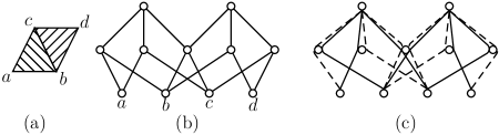
Figure 1. Example of a 2-dimensional c.c.c: (a) shows two triangles joined along a common edge. (b) shows the partially ordered set of the c.c.c corresponding to this geometric figure. (c) shows the flags of the c.c.c, drawn in two kinds of lines, showing an orientation.

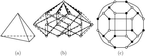
Figure 2. a three dimensional c.c.c: (a) the tetrahedron. (b) the flags drawn in two kind of lines. (c) the adjacency graph of flags.

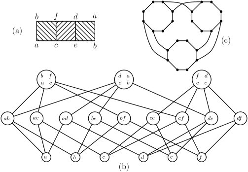
Figure 3. (a) shows the Mobius strip broken up into three squares. (b) shows the c.c.c corresponding to the Mobius strip. (c) shows the adjacency graph of flags; this graph is not bipartite.

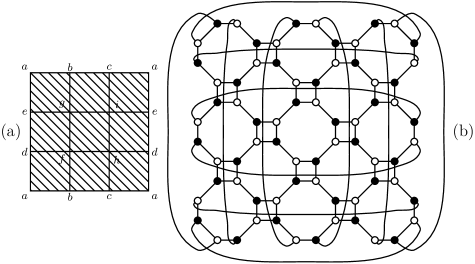
Figure 4. (a) the torus broken up into 9 squares. (b) the adjacency graph of flags.

4.3 Remark.

1. Suppose $S$ is a c.c.c with flag–connected cells. Suppose $x$ is a cell of $S$ and $y$ is a face of $x$. Then each flag below $y$ can be extended uniquely to a flag below $x$. So an orientation $\omega$ on $x$ induces an orientation $\omega|_{y}$ on $y$, defined by

   $$\omega|_{y}(\gamma)=\omega(\gamma\cup\{x\})\text{\;\; for \;\;}\gamma\in\mathcal{F}(y).$$

   It follows that, if each maximal cell of $S$ is orientable, then each cell of $S$ is orientable.

   An orientation on $S$ determines an orientation on each maximal cell of $S$. So if $S$ is orientable, with flag–connected cells, then each cell of $S$ is orientable.

2. If two cells $x_{+}$ and $x_{-}$ share a face $x$, then an orientation on $\operatorname{cl}\{x_{+},x_{-}\}$ induces two opposite orientations on $\operatorname{cl}(x)$, one coming from the orientation on $\operatorname{cl}(x_{+})$ and the other one coming from the orientation on $\operatorname{cl}(x_{-})$.

3. Notice that an orientable c.c.c must be non-singular. If an $1$–cell of $S$ has $r$ faces, or if there are $r$ maximal cells of $S$ sharing a common face, then the graph $\mathcal{F}(S)$ contains a complete graph on $r$ vertices. So $\mathcal{F}(S)$ can be bipartite only if $r\leq 2$.

4. Suppose $S$ is a non-singular c.c.c with only one maximal cell. Then an orientation on $S$ determines an orientation on the boundary of $S$.

4.4 Definition.

Let $x$ be an orientable cell of a c.c.c $S$ and $y$ be an orientable face of $x$. Let $\omega$ be an orientation on $x$ and $\mu$ be an orientation on $y$. We define,

$$s(\omega,\mu)=\begin{cases}1&\text{\;\;if\;\;}\omega|_{y}=\mu,\\ -1&\text{\;\;if\;\;}\omega|_{y}=-\mu.\end{cases}$$

If $\omega_{x}$ is an orientation on $x$ and $\omega_{y}$ is an orientation on $y$, then we write $s(x,y)=s(\omega_{x},\omega_{y})$. To determine $s(x,y)$, consider a flag $\gamma\in\mathcal{F}(x)$ of the form $\gamma=\{x>y>\dotsb\}$. Then

$$s(x,y)=\omega_{x}(\gamma)/\omega_{y}(\gamma\setminus\{x\}).$$ (1)

Since the graph $\mathcal{F}(y)$ is connected, the right hand side of equation (1) does not depend on the choice of the flag $\gamma$.

5. homology and cohomology groups

5.1.

For this section, let $S$ be a c.c.c such that each cell of $S$ is orientable. Pick an orientation on each cell $x$ of $S$, denoted by $\omega_{x}\colon\thinspace\mathcal{F}(\operatorname{cl}(x))\to\{\pm 1\}$. Given this data, we can associate a sign $s(x,y)\in\{\pm 1\}$, for each pair $x$ and $y$, where $x$ is a cell and $y$ is a face of $x$ (see 4.4). The key equation satisfied by the numbers $s(x,y)$ is given in the following lemma. Axiom (4) in the definition of a c.c.c, which is our main axiom, is used here.

5.2 Lemma.

Given the setup in section 5 so far, Let $z$ be a co-dimension $2$ facet of $x\in S$. Let $y_{+}$ and $y_{-}$ be the two cells in between $x$ and $z$, that is, $\Delta x\cap\nabla z=\{y_{+},y_{-}\}$. Then

$$s(x,y_{+})s(y_{+},z)+s(x,y_{-})s(y_{-},z)=0.$$ (2)

Proof.

Let $\gamma=\{z=z_{0}>z_{1}>\dotsb\}$ be a flag below $z$. Let $\gamma_{+}=\{x>y_{+}>z_{0}>z_{1}>\dotsb\}$ and $\gamma_{-}=\{x>y_{-}>z_{0}>z_{1}>\dotsb\}$ be the two flags below $x$ that extend $\gamma$. Then

$$s(x,y_{+})s(y_{+},z)=\frac{\omega_{x}(\gamma_{+})}{\omega_{y_{+}}(\gamma_{+}\setminus\{x\})}\cdot\frac{\omega_{y_{+}}(\gamma_{+}\setminus\{x\})}{\omega_{z}(\gamma)}=\frac{\omega_{x}(\gamma_{+})}{\omega_{z}(\gamma)}$$

Similarly $s(x,y_{-})s(y_{-},z)=\omega_{x}(\gamma_{-})/\omega_{z}(\gamma)$. Since $\gamma_{+}$ and $\gamma_{-}$ are adjacent flags in $\mathcal{F}(x)$, the lemma follows. ∎

5.3 Definition.

Now we can define chain complexes, boundary maps, homology groups et-cetera in the standard fashion. For each cell $x$ of $S$, we introduce a formal variable, denoted by $[x]$. The group of $i$–chains in $S$ with integer coefficients, denoted by $C_{i}(S)$, is the free $\mathbb{Z}$–module with basis $\{[x]\colon x\in S(i)\}$. (Of course, one can replace $\mathbb{Z}$ by other commutative rings but we shall restrict ourselves to integer coefficients). Let

$$\partial[x]=\sum_{y\in\Delta x}s(x,y)[y]\text{\;\;\;\; and \;\;\;\;}\delta[x]=\sum_{z\in\nabla x}s(z,x)[z].$$

Define the boundary map $\partial\colon\thinspace C_{i}(S)\to C_{i-1}(S)$ and the co-boundary map $\delta\colon\thinspace C_{i}(S)\to C_{i+1}(S)$ by linearly extending the above. In other words, for an $i$–chain $\sigma=\sum_{x\in S(i)}r_{x}[x]$, let

$$\partial(\sum_{x\in S(i)}r_{x}[x])=\sum_{x\in S(i)}r_{x}\partial[x]\text{\;\; and \;\;}\delta(\sum_{x\in S(i)}r_{x}[x])=\sum_{x\in S(i)}r_{x}\delta[x].$$

The image of a minimal (resp. maximal) cell under the boundary (resp. co-boundary) map is defined to be zero. If $\sigma\in C_{i}(S)$ such that $\partial\sigma=0$ (resp. $\delta\sigma=0$) we say that $\sigma$ is an $i$–cycle (resp. $i$–cocycle).

5.4 Lemma.

Given the setup in section 5 so far, one has $\partial^{2}=0$ and $\delta^{2}=0$.

Proof.

The proof follows from axiom (4) in the definition 2.2 and lemma 2. ∎

5.5 Definition.

Let $C_{i}=C_{i}(S)$. The lemma above shows that $(C_{i},\partial)$ and $(C_{i},\delta)$ are chain complexes. We define the cellular homology (resp. cellular cohomology) of $S$ to be the homology of the chain complex $(C_{i},\partial)$, (resp. $(C_{i},\delta)$).

$$H_{i}(S)=\frac{\operatorname{ker}(\partial\colon\thinspace C_{i}\to C_{i-1})}{\operatorname{im}(\partial\colon\thinspace C_{i+1}\to C_{i})}\text{\;\; and \;\;}H^{i}(S)=\frac{\operatorname{ker}(\delta\colon\thinspace C_{i}\to C_{i+1})}{\operatorname{im}(\delta\colon\thinspace C_{i-1}\to C_{i})}.$$

5.6 Remark.

  

1. To define the homology and cohomology of $S$, we need each cell of $S$ to be orientable. We do not require that $S$ is non-singular or even equidimensional. If each cell of $S$ is orientable, and $T$ is a closed subset of $S$, then each cell of $T$ is also orientable. So the homology/cohomology groups of $T$ are well defined. However $T$ need not be equidimensional or non-singular, even if $S$ were. We shall have occasion to consider homology groups of such $T$.

2. Suppose $S$ is a c.c.c with orientable cells. Given an orientation $\omega_{y}$ on each cell $y$ of $S$, we get the chain complex $(C_{\bullet},\partial)$ as defined above. Let us temporarily write $(C_{\bullet},\partial)=(C_{\bullet}^{\omega},\partial^{\omega})$ to emphasize that the chain complex depends on the choice of $\omega_{y}$’s. However, as we shall now see, choosing a different set of orientations, give an isomorphic chain complex. Let $\{\mu_{y}\colon y\in S\}$ be another set of orientations on the cells of $S$. Define $t(y)=1$ if $\omega_{y}=\mu_{y}$ and $t(y)=-1$ if $\omega_{y}=-\mu_{y}$. Then it can be easily checked that the map $[y]\mapsto t(y)[y]$ gives an isomorphism,

   $$(C_{\bullet}^{\omega},\partial^{\omega})\simeq(C_{\bullet}^{\mu},\partial^{\mu}),$$

   of chain complexes. So the homology groups do not depend on the choice of $\omega_{y}$. The same remark applies to the cohomology groups.

3. Assume that $S$ has orientable cells. Then each $1$–cell has two vertices. The zero cycles of $S$ are just linear combinations of vertices of $S$. Usually we shall assume that $\omega_{v}(\{v\})=1$ for each cell $v$ of rank zero. Under this assumption, if $v_{+}$ and $v_{-}$ are the two vertices of an $1$–cell $x$, then $s(x,v_{+})+s(x,v_{-})=0$. So two vertices $v_{1}$ and $v_{2}$ are in the same homology class if and only if they can be “joined by a sequence of $1$–cells”.

   Consider the graph $S_{\leq 1}$ whose edges correspond to the $1$–cells of $S$ and the two endpoints of an edge $x$ correspond to the two rank zero cells of $S$ below $x$. Then $H_{0}(S)$ is simply the zero-th homology of the one dimensional CW–complex $S_{\leq 1}$. Suppose the graph $S_{\leq 1}$ has $r$ connected components. Then $H_{0}(S)$ is a free abelian group of rank $r$. If one vertex is chosen from each component of the graph $S_{\leq 1}$, then $H_{0}(S)$ is freely generated by the homology classes of these $r$ vertices. In particular, if $H_{0}(S)\simeq\mathbb{Z}$, then $H_{0}(S)$ is generated by the class of any vertex of $S$.

4. Let $T$ be a closed subset of $S$. Let $C_{i}(S,T)=C_{i}(S)/C_{i}(T)$. If $\sigma\in C_{i}(T)$, then its boundary $\partial\sigma$ belongs to $C_{i-1}(T)$. Thus $\partial$ induces boundary maps $\partial_{T}^{S}\colon\thinspace C_{i}(S,T)\to C_{i-1}(S,T)$. We define the relative homology of the pair $(S,T)$ to be homology of the chain complex $(C_{i}(S,T),\partial_{T}^{S})$.

5.7 Lemma.

Let $S$ be a simplicial complex. For each simplex $\gamma=\{x_{0},\dotsb,x_{r}\}\in S$ of rank $r$, choose a total ordering, $x_{r}<_{\gamma}x_{r-1}<_{\gamma}\dotsb<_{\gamma}x_{0}$, on the set of vertices of $\gamma$. Assume that these total orderings are compatible with each other, that is, if $\gamma^{\prime}\subseteq\gamma$, then $<_{\gamma^{\prime}}$ is the restriction of $<_{\gamma}$ to the vertices of $\gamma^{\prime}$. Now consider $S$ as a combinatorial cell complex.

Then each cell of $S$ is flag–connected and there exists an orientation $\omega_{\gamma}$ on each cell $\gamma$ of $S$ such that

$$s(\gamma,\gamma\setminus\{x_{i}\})=(-1)^{i}.$$

It follows that the homology of the c.c.c $S$ (as defined in 5.5) coincides with the simplicial homology of the simplicial complex $S$ (as defined, for example, in section 3.2 of [8]).

Proof.

Let $\gamma=\{x_{0},\dotsb,x_{r}\}$ be a simplex of $S$. A total ordering, given by $x_{r}<_{\gamma}\dotsb<_{\gamma}x_{0}$, on the vertices of $\gamma$, induces an orientation on $\gamma$, as follows.

Given a flag $\Gamma=\{\gamma=\Gamma_{0}\supset\Gamma_{1}\supset\dotsb\supset\Gamma_{r}\}$ in $\operatorname{cl}(\gamma)$, one gets a permutation $P_{\gamma}(\Gamma)$ of $(r+1)$ letters, defined by $\Gamma_{i}\setminus\Gamma_{i+1}=\{x_{P_{\gamma}(\Gamma)(i)}\}$. Define $\omega_{\gamma}\colon\thinspace\mathcal{F}(\gamma)\to\{\pm 1\}$ by

$$\omega_{\gamma}(\Gamma)=\operatorname{sign}(P_{\gamma}(\Gamma)).$$

If $\Gamma$ and $\Gamma^{\prime}$ are adjacent flags below $\gamma$, then the permutations $P_{\gamma}(\Gamma)$ and $P_{\gamma}(\Gamma^{\prime})$ differ by a transposition. So $\omega_{\gamma}$ is an orientation on the cell $\gamma$. Notice that $\mathcal{F}(\gamma)$ is flag connected since the symmetric group is generated by transpositions.

To determine $s(\gamma,\gamma\setminus\{x_{0}\})$, consider the flag $\Gamma=\{\Gamma_{0}\supseteq\Gamma_{1}\supseteq\dotsb\supseteq\Gamma_{r}\}$ given by $\Gamma_{i}=\gamma\setminus\{x_{0},\dotsb,x_{i-1}\}$. Then $P_{\gamma}(\Gamma)$ and $P_{\gamma\setminus\{x_{0}\}}(\Gamma\setminus\{\gamma\})$ are both equal to the identity permutation. So

$$\omega_{\gamma}(\Gamma)=\omega_{\gamma\setminus\{x_{0}\}}(\Gamma\setminus\{\gamma\})=1.$$

It follows that $s(\gamma,\gamma\setminus\{x_{0}\})=\omega_{\gamma}(\Gamma)/\omega_{\gamma\setminus\{x_{0}\}}(\Gamma\setminus\{\gamma\})=1$. To compare $s(\gamma,\gamma\setminus\{x_{i}\})$ and $s(\gamma,\gamma\setminus\{x_{i+1}\})$, consider two adjacent flags $\Gamma_{+}$ and $\Gamma_{-}$ in $\mathcal{F}(\gamma)$, having the following form:

$$\Gamma_{+} =\{\gamma\supseteq\gamma\setminus\{x_{i}\}\supseteq\gamma\setminus\{x_{i},x_{i+1}\}\supseteq\dotsb\},$$

$$\Gamma_{-} =\{\gamma\supseteq\gamma\setminus\{x_{i+1}\}\supseteq\gamma\setminus\{x_{i},x_{i+1}\}\supseteq\dotsb\}.$$

Since $\Gamma_{+}$ and $\Gamma_{-}$ are adjacent flags, we have $\omega_{\gamma}(\Gamma_{+})=-\omega_{\gamma}(\Gamma_{-})$. On the other hand, the flags $\Gamma_{+}\setminus\{\gamma\}\in\mathcal{F}(\gamma\setminus\{x_{i}\})$ and $\Gamma_{-}\setminus\{\gamma\}\in\mathcal{F}(\gamma\setminus\{x_{i+1}\})$ correspond to the same permutation. Hence $\omega_{\gamma\setminus\{x_{i}\}}(\Gamma_{+}\setminus\{\gamma\})=\omega_{\gamma\setminus\{x_{i+1}\}}(\Gamma_{-}\setminus\{\gamma\})$. It follows that $s(\gamma,\gamma\setminus\{x_{i}\})$ and $s(\gamma,\gamma\setminus\{x_{i+1}\})$ have opposite signs. ∎

6. Stellar subdivision

We would like to show that if $S$ is a manifold–like c.c.c with orientable and acyclic cells, then the homology of $S$ is isomorphic to that of its barycentric subdivision $S^{(1)}$. It is easy to write down a chain map from the $i$–chains of $S$ to those of $S^{(1)}$. But it seems difficult to show directly that this map induces isomorphism of homology groups, since the cell structure of $S^{(1)}$ is very different from the cell structure of $S$. For this purpose, we want to break up the transition from $S$ to $S^{(1)}$ into many successive “stellar subdivisions” or “stellar refinements”. In each step, the cell structure is only “locally” modified. This makes it easier to compare the homology groups in successive steps. Stellar subdivisions of simplicial and cell complexes arise in many places in literature, for example, see [6], [8].

6.1 Definition.

Let $x$ be a cell of a c.c.c $S$. Define the star of $x$ to be

$$\operatorname{star}(x)=\operatorname{cl}(U(x)).$$

We also define $M(x)=\operatorname{star}(x)\setminus U(x)$ and $\tilde{M}(x)=M(x)\cup\{\emptyset\}$ (see figure 5). Both $\operatorname{star}(x)$ and $M(x)$ are closed subsets of $S$. So these are sub–c.c.c’s of $S$. When there is a possibility of confusion, we write $\operatorname{star}_{S}(x)$ and $M_{S}(x)$. Say that $S$ is a star around $x$, if $\operatorname{star}_{S}(x)=S$.

Figure 5.

6.2 Definition.

Let $S$ be a c.c.c and $x\in S(i)$ for some $i\geq 1$. We want to define a new c.c.c $S^{x}$, to be called the stellar subdivision of $S$ at $x$. (To get the idea, look at the examples in figure 6). For each $y\in\tilde{M}(x)$, introduce new cells $C_{x}(y)$, to be called the cone over $y$ with vertex at $x$. Define $S^{x}(0)=S(0)\cup\{C_{x}(\emptyset)\}$ and

$$S^{x}(r)=\{y\in S(r)\colon y\ngeq x\}\cup\{C_{x}(y):y\in\tilde{M}(x)(r-1)\},$$

with the convention that $\tilde{M}(x)(-1)=\{\emptyset\}$. There are two kinds of cells in $S^{x}$. The first kind consists of the cells of $S\setminus U_{S}(x)$; these will be called the old cells. The second kind consists of the cones; these will be called the new cells.

Next, we define the partial order on $S^{x}$. Given two cells $y$ and $z$ of $S^{x}$, the relation $y\leq_{S^{x}}z$ holds if and only if one of the following conditions hold.

• Both $y$ and $z$ are old cells and $y\leq_{S}z$.

• $y$ is an old cell, $z=C_{x}(z^{\prime})$ is a new cell and $y\leq_{S}z^{\prime}$.

• Both $y=C_{x}(y^{\prime})$ and $z=C_{x}(z^{\prime})$ are new cells and $y^{\prime}\leq_{S}z^{\prime}$.

We shall check in a moment that $S^{x}$ is a c.c.c. If $T$ is obtained from $S$ by successive stellar refinements, then we say that $T$ is a refinement of $S$.

Figure 6. (a) shows a two dimensional c.c.c $S$, the stellar subdivision $S^{x}$ at the $1$–cell $x$ joining the square and the pentagon and the stellar subdivision $S^{y}$ at the 2-cell $y$. (b) shows a three dimensional c.c.c $T$ and it subdivision $T^{z}$, where the 2-cell $z$ is the square in the middle. The new vertices, namely $C_{x}(\emptyset)$, $C_{y}(\emptyset)$ and $C_{z}(\emptyset)$, are marked with a circle.

6.3 Remark.

1. Let $T=\operatorname{star}_{S}(x)$ and $M(x)=M_{S}(x)=M_{T}(x)$. There is a canonical isomorphism: $\operatorname{star}_{S}(x)^{x}\simeq\operatorname{star}_{S^{x}}(C_{x}(\emptyset))$. On both sides, the $r$–cells are

   $$M(x)(r)\cup\{C_{x}(y)\colon y\in\tilde{M}(x)(r-1)\}.$$

   On both sides, the partial order and rank are defined in the same way. We shall often identify $\operatorname{star}_{S}(x)^{x}$ as a sub-c.c.c of $S^{x}$, via the above isomorphism.

2. Taking a stellar refinement at $x$ only changes the cell structure “around $x$”. More precisely, $\operatorname{star}_{S}(x)\subseteq S$ is replaced by $\operatorname{star}_{S}(x)^{x}\simeq\operatorname{star}(C_{x}(\emptyset))\subseteq S^{x}$. The rest of the cell structure remains unchanged.

3. The cells in $U(x)\subseteq S$ “die” in the process of stellar subdivision at $x$. The rest of the cells of $S$ “survive” as cells of $S^{x}$; these are the old cells. Finally, for each cell $y\in\tilde{M}(x)$, a cell called $C_{x}(y)$ is “born”; these are the new cells. For later use, we note the following.

   • There are no new cells below an old cell.

   • Among the faces of $C_{x}(y)$, there is only one old cell, namely $y$ itself.

4. While defining $S^{x}$, we have assumed that the rank of $x$ is atleast one, because this is the only case we shall need. However, the definition makes sense even when $x$ is a cell of rank zero. In this case the vertex $x$ gets replaced by the vertex $C_{x}(\emptyset)$.

6.4 Lemma.

Let $S$ be a c.c.c and $x$ be a cell of $S$ of rank at-least one. Then,
(a) $S^{x}$ is a c.c.c.
(b) If $S$ is equidimensional, of dimension $n$, then so is $S^{x}$.
(c) If each $1$–cell of $S$ has two vertices, then the same is true for each $1$–cell of $S^{x}$.
(d) Suppose $S$ is equidimensional, of dimension $n$. If there are at-most two (resp. exactly two) $n$–cells above each $(n-1)$–cell of $S$, then the same is true for $S^{x}$.
(e) If $S$ is non-singular (resp. manifold–like), then $S^{x}$ is non-singular (resp. manifold–like).

The proof, given in appendix A.1, is easy but a little tedious. It is mainly because we have to separate the argument into cases, depending on whether the cell of $S^{x}$ we are dealing with is a cone or not.

We shall have occasion to consider repeated stellar subdivision of a c.c.c. We shall write $(X^{x})^{y}=X^{xy}$. The c.c.c one obtains by repeated stellar subdivision depends, in general, on the order in which the subdivision points are chosen. However, we have the following result.

6.5 Lemma.

Let $X$ be a c.c.c and $\{x_{1},\dotsb,x_{k}\}\subseteq X$ such that $U_{X}(x_{i})\cap U_{X}(x_{j})=\emptyset$ for all $i\neq j$. Then the refinement $X_{(k)}=X^{x_{1}x_{2}\dotsb x_{k}}$ has the following description:

$$X_{(k)}=\operatorname{\cup}_{j=1}^{k}\{C_{x_{j}}(v)\colon v\in\tilde{M}_{X}(x_{j})\}\cup\bigl{(}X\setminus\operatorname{\cup}_{j=1}^{k}U_{X}(x_{j})\bigr{)}.$$

As before, the cells of the form $C_{x_{j}}(v)$ are called the new cells and the rest are called the old cells. The partial order on $X_{(k)}$ is defined by the following rules. One has $\alpha\leq_{X_{(k)}}\beta$ if and only if one of the following three conditions hold:

• both $\alpha$ and $\beta$ are old and $\alpha\leq_{X}\beta$.

• $\alpha$ is old, $\beta=C_{x_{j}}(\beta^{\prime})$ is new and $\alpha\leq_{X}\beta^{\prime}$.

• both $\alpha$ and $\beta$ are new, there is a $j$ between $1$ and $k$ such that $\alpha=C_{x_{j}}(\alpha^{\prime})$, $\beta=C_{x_{j}}(\beta^{\prime})$ and $\alpha^{\prime}\leq_{X}\beta^{\prime}$.

It follows from this description that there are no old cells above a new cell and $X_{(k)}$ does not depend on the order of subdivision.

The proof is given in appendix A.2.

Suppose $X$ is a c.c.c such that each cell of $X$ is orientable but $X$ itself is not orientable. We will need to consider the homology groups of such an $X$ and of its stellar subdivision $X^{x}$. We need the following lemma to make sure that the homology of $X^{x}$ is well defined.

6.6 Lemma.

Let $X$ be a c.c.c and let $x$ be a cell of $X$.

(a) If each cell of $X$ is flag-connected, then each cell of $X^{x}$ is flag connected.

(b) If each the cell of $X$ is orientable, then each cell of $X^{x}$ is also orientable. More precisely, one has the following: Let $y\in M_{X}(x)$ with $\operatorname{rk}(y)=n-1$. Let $S=\operatorname{cl}_{X}(y)\subseteq X$ and $S^{\prime}=\operatorname{cl}(C_{x}(y))\subseteq X^{x}$. Given a flag $\gamma\in\mathcal{F}(S^{\prime})$, there is an $i\geq 0$ such that

$$\gamma=\{C_{x}(y_{0})>C_{x}(y_{1})>\dotsb>C_{x}(y_{i})>y_{i}>y_{i+2}>y_{i+3}>\dotsb>y_{n}\}$$

where $y_{0}=y$ and $y_{j}\in S$, with the exception that $y_{n}=\emptyset$ if $i=n$. We let $l(\gamma)=i$ and

$$\tilde{\gamma}=\{y_{0}>y_{1}>\dotsb>y_{i}>y_{i+2}>y_{i+3}>\dotsb>y_{n}\}\in\mathcal{F}(S),$$

with the convention that $y_{n}=\emptyset$ is omitted if $i=n$. If $\omega_{y}$ is an orientation on $S=\operatorname{cl}_{X}(y)$, then $\omega_{S^{\prime}}$, defined by

$$\omega_{S^{\prime}}(\gamma)=(-1)^{l(\gamma)}\omega_{y}(\tilde{\gamma}),$$

is an orientation on $S^{\prime}=\operatorname{cl}(C_{x}(y))$.

The proof is given in appendix A.3.

6.7 Definition.

Let $S$ be a c.c.c with orientable cells and $x\in S$. Fix an orientation $\omega_{z}$ for each cell $z\in S$. Given this data, we define an orientation on each cell of $S^{x}$ as follows. If $z\in S^{x}$ is an old cell, then $\mathcal{F}_{S}(z)=\mathcal{F}_{S^{x}}(z)$. So $\omega_{z}$ is already defined. If $C_{x}(y)$ is a cone in $S^{x}$, then choose $\omega_{C_{x}(y)}$ as prescribed by lemma 6.6(b). For a flag $\gamma$ with top two cells $C_{x}(y)$ and $y$, we have, in the notation of lemma 6.6, $\tilde{\gamma}=\gamma\setminus C_{x}(y)$ and $l(\gamma)=0$, so $\omega_{C_{x}(y)}(\gamma)=\omega_{y}(\gamma\setminus\{C_{x}(y)\})$. In other words, in the notation of 4.4, we have

$$s(C_{x}(y),y)=1.$$ (3)

Suppose $y\in M_{S}(x)$ and $z$ is a face of $y$. So $z$ is a co-dimension 2 facet of $C_{x}(y)$. The two cells in between $C_{x}(y)$ and $z$ are $C_{x}(z)$ and $y$. From lemma 2, one has,

$$s(C_{x}(y),C_{x}(z))s(C_{x}(z),z)=-s(C_{x}(y),y)s(y,z).$$

Since $s(C_{x}(u),u)=1$ for all $u$, it follows that

$$s(C_{x}(y),C_{x}(z))=-s(y,z).$$ (4)

6.8 Lemma.

Let $S$ be a c.c.c with orientable cells and $x\in S$. For each $w\in S$, let $\Delta_{1}w=\Delta w\setminus U(x)$ and $\Delta_{2}w=\Delta w\cap U(x)$. Define

$$\varphi([w])=\begin{cases}\sum\limits_{y\in\Delta_{1}w}s(w,y)[C_{x}(y)]&\text{if \;}w\in U(x),\\ [w]&\text{otherwise.}\end{cases}$$

Then $\varphi$ defines a chain map $(C_{\bullet}(S),\partial)\to(C_{\bullet}(S^{x}),\partial)$ and hence induces an homomorphism $H_{i}(\varphi)\colon\thinspace H_{i}(S)\to H_{i}(S^{x})$.

Proof.

Suppose $w\in U(x)$ and $y\in\Delta_{1}(w)$. Let $Z$ be the set of co-dimension $2$ facets of $w$, that are not greater than or equal to $x$. From the description of partial order on $S^{x}$ and equations (3) and (4), we have,

$$\partial(C_{x}(y))=[y]-\sum_{z\in\Delta y}s(y,z)[C_{x}(z)].$$

It follows that

$$\partial(\varphi[w])=\sum_{y\in\Delta_{1}w}s(w,y)\partial[C_{x}(y)]=\sum_{y\in\Delta_{1}w}s(w,y)[y]-\sum_{z\in Z}\Bigl{[}\sum_{y\in\nabla z\cap\Delta_{1}w}s(w,y)s(y,z)\Bigr{]}[C_{x}(z)].$$

In the second term of the final expression, we are summing over all pairs $(y,z)$ such that $y\in\Delta w$, $z\in\Delta y$ and $y\notin U(x)$. So the set of $z$ that appear in the expression are in $Z$.

Given $z\in Z$, let $y_{+}$ and $y_{-}$ be the two cells in between $w$ and $z$. Without loss, we may assume that $y_{+}\notin U(x)$. We may write $Z$ as a disjoint union $Z=Z_{1}\cup Z_{2}$, where $Z_{1}$ (resp. $Z_{2}$) consists of those $z\in Z$, such that $y_{-}\in U(x)$ (resp. $y_{-}\notin U(x)$) (see figure 7).

Figure 7. the relevant cells around $z\in Z_{1}$

For $z\in Z_{2}$, we have $\sum_{y\in\nabla z\cap\Delta_{1}w}s(w,y)s(y,z)=s(w,y_{+})s(y_{+},z)+s(w,y_{-})s(y_{-},z)=0$. It follows that

$$\partial(\varphi[w])=\sum_{y\in\Delta_{1}w}s(w,y)[y]-\sum_{z\in Z_{1}}s(w,y_{+})s(y_{+},z)[C_{x}(z)].$$

To compute $\varphi(\partial[w])$, note that, if $y\neq y^{\prime}$ are two cells in $\Delta_{2}w$, then $\Delta_{1}y\cap\Delta_{1}y^{\prime}=\emptyset$ and $\cup_{y\in\Delta_{2}w}\Delta_{1}y=Z_{1}$. It follows that

$$\varphi(\partial[w])=\sum_{y\in\Delta_{1}w\cup\Delta_{2}w}s(w,y)\varphi[y]=\sum_{y\in\Delta_{1}w}s(w,y)[y]+\sum_{z\in Z_{1}}s(w,y_{-})s(y_{-},z)[C_{x}(z)].$$

Using lemma 2 once more, we see that $\partial\circ\varphi=\varphi\circ\partial$. ∎

7. Lemmas on vanishing of homology groups

7.1 Definition.

A c.c.c $S$ with orientable cells is acyclic if $H_{i}(S)=0$ for $i>0$ and $H_{0}(S)\simeq\mathbb{Z}$. As remarked in 4.3(3), in such a situation, $H_{0}(S)$ is generated by the homology class of any vertex of $S$. We say that $x$ is an acyclic cell if $\operatorname{cl}(x)$ is acyclic. In this section we want to show that, if the cells of $S$ are acyclic, then the cells of $S^{x}$ are acyclic and $H_{\bullet}(S)\simeq H_{\bullet}(S^{x})$.

7.2 Lemma.

Let $T$ be a c.c.c with orientable cells. Let $x$ and $y$ be two cells of $T$ such that $y\in M(x)$. Let $S=\operatorname{cl}_{S}(y)$ and $S^{\prime}=\operatorname{cl}_{S^{x}}(C_{x}(y))$. Let $j\colon\thinspace S\to S^{\prime}$ be the inclusion map, $j(z)=z$. Then one has the following:
(a) The induced map on homology, $j_{*}\colon\thinspace H_{i}(S)\to H_{i}(S^{\prime})$, is the zero map, for $i\geq 1$.
(b) If $y$ is acyclic, then so is $C_{x}(y)$.
(c) If all the cells of $T$ are acyclic, then all the cells of $T^{x}$ are also acyclic.

Proof.

Let $z$ be a facet of $y$. Since $x$ is not a facet of $y$, it is not a facet of $z$ either. So $z$ remains a cell in $S^{x}$. So $j(z)=z$ defines an injective chain map from $C_{i}(S)$ to $C_{i}(S^{\prime})$. We shall identify $C_{\bullet}(S)$ as a sub-chain complex of $C_{\bullet}(S^{\prime})$ via the function $j$. Also, note that $z\vee x$ exists, so $C_{x}(z)$ is a cell of $S^{\prime}$. Thus, the $r$–cells of $S^{\prime}$ are the $r$–cells of $S$ and the cones on the $(r-1)$–cells of $\tilde{S}$. (Recall that $\tilde{S}(r)=S(r)$ for $r\geq 0$ and $\tilde{S}(-1)=\{\emptyset\}$.)

As $\Delta(z)\cap U(x)=\emptyset$ for each facet $z$ of $y$, using equation (4), the boundary of a cone is given by

$$\partial([C_{x}(z)])=[z]-\sum_{w\in\Delta z}s(z,w)[C_{x}(w)].$$

Let $C_{\bullet}(\tilde{S})$ be the chain complex $C_{\bullet}(S)$ augmented by ${C}_{-1}(S)=\mathbb{Z}[\emptyset]$:

$$\dotsb\to C_{i}(\tilde{S})\to C_{i-1}(\tilde{S})\to\dotsb\to C_{1}(\tilde{S})\to C_{0}(\tilde{S})\to C_{-1}(\tilde{S})\to 0,$$

where the boundary map $C_{0}(\tilde{S})\to C_{-1}(\tilde{S})$ sends $[x]$ to $[\emptyset]$ for each vertex $x$ of $S$. The $i$–th homology of this chain complex will be denoted by $H_{i}(\tilde{S})$ for $i\geq-1$. Let

$$h_{i}\colon\thinspace C_{i}(\tilde{S})\to C_{i+1}(S^{\prime})$$

be the linear map induced by $[z]\mapsto[C_{x}(z)]$. From the above formula for the boundary of a cone, one gets $(h\circ\partial+\partial\circ h)([z])=[z]$, which implies part (a).

Recall that, we have identified $C_{i}(S)$ as a sub-complex of $C_{i}(S^{\prime})$, via the inclusion $j$. The function $h_{i}$ above induces a map $\bar{h}_{i}\colon\thinspace C_{i}(\tilde{S})\to C_{i+1}(S^{\prime})/C_{i+1}(S)$, satisfying $\bar{h}\circ\partial+\partial\circ\bar{h}=0$, showing that $(-1)^{i}\bar{h}_{i}\colon\thinspace C_{i}(\tilde{S})\to C_{i+1}(S^{\prime})/C_{i+1}(S)$ is a chain map. The map $\bar{h}_{i}$ is a bijection on the level of chains, since $C_{i+1}(S^{\prime})=C_{i+1}(S)\oplus h_{i}(C_{i}(\tilde{S}))$ as abelian groups. So the chain complex $C_{\bullet}(S^{\prime})/C_{\bullet}(S)$ is isomorphic to $C_{\bullet-1}(\tilde{S})$. One has the following exact sequence of chain complexes:

$$0\rightarrow C_{i}(S)\rightarrow C_{i}(S^{\prime})\rightarrow C_{i}(S^{\prime})/C_{i}(S)\simeq C_{i-1}(\tilde{S})\rightarrow 0.$$

By taking the long exact sequence of homology groups, one gets $H_{i}(S^{\prime})=0$ for $i\geq 2$, since $H_{i}(S)=0$ and $H_{i-1}(\tilde{S})=H_{i-1}(S)=0$. The end of this long exact sequence has the form,

$$0\rightarrow H_{1}(S)\to H_{1}(S^{\prime})\to H_{0}(\tilde{S})\to H_{0}(S)\to H_{0}(S^{\prime})\to H_{-1}(\tilde{S})\to 0.$$

By remark 4.3(3), $H_{0}(S)\simeq\mathbb{Z}$ is generated by the class of any vertex of $S$. So

$$\partial(C_{1}(S))=\operatorname{span}\{[u]-[v]:u,v\in S(0)\}.$$

So $\partial(C_{1}(S))$ is the kernel of the map $C_{0}(S)\to C_{-1}(S)$. Thus $H_{0}(\tilde{S})=0$. Also $H_{-1}(\tilde{S})=0$. It follows that $H_{1}(S^{\prime})\simeq H_{1}(S)=0$ and $H_{0}(S^{\prime})\simeq H_{0}(S)\simeq\mathbb{Z}$. This finishes the proof of part (b). Part (c) follows from part (b). ∎

7.3 Lemma.

(a) Let $S$ be a c.c.c with orientable cells and $x\in S$. Assume that $S$ is a star around $x$, that is, $\operatorname{star}_{S}(x)=S$. Then $S^{x}$ is acyclic.
(b) Let $X$ be a c.c.c with orientable cells and $x\in X$. Then $\operatorname{star}(C_{x}(\emptyset))\subseteq X^{x}$ is acyclic.

As remarked in 6.3(1), there is a canonical isomorphism, $\operatorname{star}_{X^{x}}(C_{x}(\emptyset))\simeq\operatorname{star}_{X}(x)^{x}$. So part (b) follows from part (a). The proof of part (a), given in appendix A.4, is similar to the proof of lemma 7.2.

7.4 Lemma.

Let $S$ be a c.c.c with orientable acyclic cells. If $S$ is a star around $x$, then $S$ is acyclic. In particular $\operatorname{star}(x)$ is acyclic for all $x\in S$. (For the proof, it is important to note that we do not assume $S$ to be equidimensional or nonsingular).

Proof.

Let $\dim(S)=n$. If $x$ is a maximal cell of $S$, then $S=\operatorname{star}(x)=\operatorname{cl}(x)$ is acyclic, by assumption. For a non-maximal cell $x$, let $t_{1},\dotsb,t_{k}$ be the maximal cells above $x$ arranged in decreasing order of rank, that is, $\operatorname{rk}(t_{1})\geq\operatorname{rk}(t_{2})\geq\dotsb\geq\operatorname{rk}(t_{k})$. Let $\rho_{S}(x)=\operatorname{rk}(t_{1})-\operatorname{rk}(x)$. The proof is by induction on $\rho_{S}(x)$.

Though logically it is not necessary, we first prove the lemma in the case $\rho_{S}(x)=1$, to illustrate the idea. Since $x$ is not a maximal cell, one has $\operatorname{rk}(t_{i})=\operatorname{rk}(x)+1$. In other words, $\nabla x=\{t_{1},\dotsb,t_{k}\}$. By induction on $j$, we show that $T_{j}=\operatorname{cl}\{t_{1},\dotsb,t_{j}\}$ is acyclic. The case $j=1$ is a part of assumption. Assume now, that $T_{j-1}$ is acyclic. Since $T_{j}=T_{j-1}\cup\operatorname{cl}(t_{j})$ and $T_{j-1}\cap\operatorname{cl}(t_{j})=\operatorname{cl}(x)$, one has the following exact sequence of chain complexes:

$$0\to C_{\bullet}(\operatorname{cl}(x))\xrightarrow[]{p}C_{\bullet}(T_{j-1})\oplus C_{\bullet}(\operatorname{cl}(t_{j}))\xrightarrow[]{q}C_{\bullet}(T_{j})\to 0,$$

where $p(\lambda)=(\lambda,-\lambda)$ and $q(\mu,\sigma)=\mu+\sigma$. By taking the long exact sequence of homology groups, one gets $H_{i}(T_{j})=0$ for $i\geq 2$. Further, looking at the end of the long exact sequence, one has,

$$0\to H_{1}(T_{j})\to H_{0}(\operatorname{cl}(x))\xrightarrow[]{H_{0}(p)}H_{0}(T_{j-1})\oplus H_{0}(\operatorname{cl}(t_{j}))\to H_{0}(T_{j})\to 0.$$

Let $v$ be any vertex of $x$. Then, by remark 4.3(3), $[v]$ generates $H_{0}(\operatorname{cl}(x))$ and $H_{0}(\operatorname{cl}(t_{j}))$. The map $H_{0}(p)\colon\thinspace H_{0}(\operatorname{cl}(x))\to H_{0}(T_{j-1})\oplus H_{0}(\operatorname{cl}(t_{j}))$ sends $[v]$ to $([v],-[v])$. Since $-[v]\in H_{0}(\operatorname{cl}(t_{j}))$ is non-zero, the map $H_{0}(p)$ is injective. It follows that $H_{1}(T_{j})=0$ and $H_{0}(T_{j})\simeq\mathbb{Z}$. This completes the proof for $\rho_{S}(x)=1$.

Now, let $\rho_{S}(x)=r$. Assume that the lemma is true for $\rho_{S}(x)<r$. By induction on $j$, we show that $T_{j}=\operatorname{cl}\{t_{1},\dotsb,t_{j}\}$ is acyclic. The case $j=1$ is again a part of assumption. Now assume that $T_{j-1}$ is acyclic. One has $T_{j}=T_{j-1}\cup\operatorname{cl}(t_{j})$. Let $K=T_{j-1}\cap\operatorname{cl}(t_{j})$ . The c.c.c $K$ is a star around $x$ with $\operatorname{dim}(K)<\operatorname{rk}(t_{j})$, so

$$\rho_{K}(x)<\operatorname{rk}(t_{j})-\operatorname{rk}(x)\leq r.$$

Since the lemma is assumed to be true for $\rho_{S}(x)<r$, we get that $K$ is acyclic. As before, one has the exact sequence

$$0\to C_{\bullet}(K)\xrightarrow[]{p}C_{\bullet}(T_{j-1})\oplus C_{\bullet}(\operatorname{cl}(t_{j}))\xrightarrow[]{q}C_{\bullet}(T_{j})\to 0.$$

The result follows by taking the long exact sequence of homology groups. ∎

7.5 Proposition.

Assume that $X$ is a c.c.c with orientable and acyclic cells. Let $x\in X$. Then the map $H_{\bullet}(\varphi)\colon\thinspace H_{\bullet}(X)\to H_{\bullet}(X^{x})$, defined in 6.8, is an isomorphism.

Proof.

From lemma 6.8 we have a chain map $\varphi\colon\thinspace C_{\bullet}(X)\to C_{\bullet}(X^{x})$. Let $S=\operatorname{star}_{X}(x)$. We shall identify $S^{x}$ as a sub-complex of $X^{x}$ via the identification $S^{x}\simeq\operatorname{star}_{X^{x}}(C_{x}(\phi))$ given in 6.3(1). The map $\varphi$ fits into the following commutative diagram of chain complexes:

The horizontal maps on the right are the quotient maps. One checks from the definitions that both $C_{i}(X)/C_{i}(S)$ and $C_{i}(X^{x})/C_{i}(S^{x})$ can be identified with the free abelian group on the cells of $(X\setminus S)$ and the map $\bar{\varphi}$ acts as identity on these cells. Thus $\bar{\varphi}$ is a chain isomorphism, so $H_{\bullet}(\bar{\varphi})\colon\thinspace H_{\bullet}(X,S)\to H_{\bullet}(X^{x},S^{x})$ is an isomorphism.

Next, note that $S$ and $S^{x}$ are acyclic by lemma 7.4 and 7.3 respectively. It follows that $H_{\bullet}(\varphi|_{S})$ is an isomorphism. Taking the diagram of homology groups corresponding to the above commutative diagram of chain complexes and applying the five lemma, it follows that $H_{\bullet}(\varphi)\colon\thinspace H_{\bullet}(X)\to H_{\bullet}(X^{x})$ is an isomorphism. ∎

8. Barycentric subdivision of a c.c.c

Recall, from 4.1, the definition of the barycentric subdivision of a c.c.c $S$, denoted by $S^{(1)}$.

8.1 Remark.

If $S$ is equidimensional, of dimension $n$, then the same holds for $S^{(1)}$. The $n$–cells of $S^{(1)}$ correspond to the flags in $S$. The other cells of $S^{(1)}$ correspond to totally ordered subsets of $S$, that is, “partial flags” in $S$. If $S$ is non-singular, then it is easy to see that $S^{(1)}$ is non-singular.

8.2 Lemma.

Each cell of $S^{(1)}$ is flag connected and has an orientation such that, for $\gamma=\{x_{0}>x_{1}>\dotsb>x_{r}\}\in S^{(1)}(r)$, one has $s(\gamma,\gamma\setminus\{x_{i}\})=(-1)^{i}$.

Proof.

The lemma follows from 5.7, once we note that there is a compatible family of total ordering on the vertices of each cell $\gamma\in S^{(1)}$, coming from the partial order on $S$. ∎

8.3 Lemma.

Let $S$ be a c.c.c with orientable cells. For each cell $x\in S$, choose an orientation $\omega_{x}\colon\thinspace\mathcal{F}(x)\to\{\pm 1\}$. Choose orientations on the cells of $S^{(1)}$ as prescribed by lemma 8.2. If $x\in S(r)$, then a flag $\gamma\in\mathcal{F}(x)$ determines an $r$–cell in $S^{(1)}$ and thus an $r$–chain $[\gamma]$. There is a chain map $\Phi\colon\thinspace C_{\bullet}(S)\to C_{\bullet}(S^{(1)})$, given by

$$\Phi([x])=\sum_{\gamma\in\mathcal{F}(x)}\omega_{x}(\gamma)[\gamma].$$

Proof.

To check that $\Phi$ is a chain map, we first calculate $\partial_{S^{(1)}}(\Phi[x])$.

$$\partial_{S^{(1)}}(\Phi[x])=\sum_{\gamma\in\mathcal{F}(x)}\omega_{x}(\gamma)\partial_{S^{(1)}}[\gamma]=\sum_{\gamma\in\mathcal{F}(x)}\omega_{x}(\gamma)\sum_{\xi\in\Delta\gamma}s(\gamma,\xi)[\xi].$$

Consider a “partial flag” $\xi$ appearing in the final expression. Suppose $\xi$ is of the form $\{x=x_{0}>x_{1}>\dotsb>x_{i-1}>x_{i+1}>\dotsb>x_{r}\}$ for some $i>0$, where $x_{j}\in S(r-j)$. Then there are two adjacent flags $\gamma_{+}$ and $\gamma_{-}$ in $\mathcal{F}(x)$, such that $\xi$ is a face of $\gamma_{\pm}$. We have $\omega_{x}(\gamma_{+})=-\omega_{x}(\gamma_{-})$ and $s(\gamma_{+},\xi)=s(\gamma_{-},\xi)=(-1)^{i}$ (by lemma 8.2). So, in the expression for $\partial_{S^{(1)}}(\Phi[x])$, the coefficient of $[\xi]$ vanishes.

Let $\xi$ be a “partial flag” that is not of the above form. Then $\xi$ is of the form $\{x_{1}>x_{2}>\dotsb>x_{r}\}$, where $x_{j}$ is a cell below $x$ of rank $(r-j)$. That is, $\xi$ is a flag in $\operatorname{cl}(\Delta x)$. The only flag $\gamma\in\mathcal{F}(x)$, that has $\xi$ as a face, is $\gamma=\{x=x_{0}>x_{1}>\dotsb>x_{r}\}$. Lemma 8.2 implies $s(\gamma,\xi)=1$. It follows that

$$\partial_{S^{(1)}}(\Phi[x])=\sum_{\xi\in\mathcal{F}(\operatorname{cl}(\Delta x))}\omega_{x}(\xi\cup\{x\})[\xi]=\sum_{y\in\Delta x}s(x,y)\sum_{\xi\in\mathcal{F}(y)}\omega_{y}(\xi)[\xi]=\Phi(\partial_{S}[x]).$$

So $\Phi$ induces a map $H_{i}(\Phi)\colon\thinspace H_{i}(S)\to H_{i}(S^{(1)})$. ∎

Suppose $S$ is a c.c.c of dimension $n$. Let $y_{1},\dotsb,y_{N}$ be an ordering of all the cells of $S$ of rank at-least one, such that $\operatorname{rk}(y_{1})\geq\operatorname{rk}(y_{2})\geq\dotsb\geq\operatorname{rk}(y_{N})$. We shall now prove that the first barycentric subdivision of $S$ can be obtained by taking successive stellar subdivision at $y_{1},y_{2},\dotsb,y_{N}$, in that order. Because of lemma 6.5, it does not matter how the cells having the same rank are ordered. (See proposition 2.23 of [8] for the same result for simplicial complexes.) We shall use the following abbreviation and convention:

$$C_{w_{j}\dotsb w_{1}}(v)=C_{w_{j}}(C_{w_{j-1}}(\dotsb C_{w_{1}}(v))).\text{\; If $j=0$, then \;}C_{\emptyset}(v)=v.$$

8.4 Lemma.

Let $S$ be a manifold–like c.c.c of dimension $n$ with orientable cells. Let $x^{r}_{1},x^{r}_{2},\dotsb,x^{r}_{k_{r}}$ be the set of $r$–cells of $S$. Starting with $T_{n+1}=S$, we shall define $T_{r}$ for $n+1\geq r\geq 1$, by backward induction on $r$. Having defined $T_{n+1},T_{n},\dotsb,T_{r+1},$ we claim that each $r$–cell of $S$ survive as a cell of $T_{r+1}$ and we define

$$T_{r}=T_{r+1}^{x_{1}^{r}x_{2}^{r}\dotsb x_{k_{r}}^{r}}.$$

Then one has the following:
$(\mathcal{A}(r))$ The cells of $T_{r}$ have the form $C_{u_{j}u_{j-1}\dotsb u_{1}}(v)$, where $0\leq j\leq n-r+1$, $u_{i}\in S$ and $v\in S\cup\{\emptyset\}$. More precisely,

$$T_{r}=\bigcup_{j=0}^{n-r+1}\{C_{u_{j}u_{j-1}\dotsb u_{1}}(v)\colon v<u_{j}<u_{j-1}\dotsb<u_{1},\operatorname{rk}(v)<r,\operatorname{rk}(u_{j-i})\geq r+i\}.$$

$(\mathcal{B}(r))$ The cells greater than or equal to $C_{w_{j}\dotsb w_{1}}(t)$ in $T_{r+1}$ are the cells of the form $C_{y_{k}\dotsb y_{1}}(v)$ where $t\leq v$ and $\{w_{j}<w_{j-1}<\dotsb<w_{1}\}$ is an ordered subset of $\{y_{k}<y_{k-1}<\dotsb<y_{1}\}$.
$(\mathcal{C}(r))$ Consider $t\in S(r)$ as a cell of $T_{r+1}$. The cells of $T_{r+1}$ that are greater than or equal to $t$ are those of the form $C_{u_{j}u_{j-1}\dotsb u_{1}}(t)$, $j\geq 0$. Thus, if $t$ and $t^{\prime}$ are two distinct $r$–cells of $S$, then $U_{T_{r+1}}(t)\cap U_{T_{r+1}}(t^{\prime})=\emptyset$. Consequently $(T_{r+1})^{tt^{\prime}}\simeq(T_{r+1})^{t^{\prime}t}$.
$(\mathcal{D})$ The c.c.c $T_{1}$ is canonically isomorphic to the first barycentric subdivision $S^{(1)}$. Under this isomorphism, The cell $C_{v_{1}v_{2}\dotsb v_{r}}(v_{0})\in T_{1}$ corresponds to the cell $\{v_{0}<v_{1}<\dotsb<v_{r}\}\in S^{(1)}$.

In the statement $\mathcal{A}(r)$ The proof is given in A.5. However, it is best to work out a few examples in dimension 2 and 3 to convince oneself of the validity of the statement.

8.5 Proposition.

Let $S$ be a manifold–like c.c.c of dimension $n$, with orientable and acyclic cells. Then $H_{\bullet}(S)\simeq H_{\bullet}(S^{(1)})$.

Proof.

By lemma 8.4, the first barycentric subdivision $S^{(1)}$ is obtained from $S$ by a sequence of successive stellar subdivisions. The property of having orientable and acyclic cells, is preserved under stellar subdivision, by lemma 6.6 and 7.2 respectively. The result now follows from repeated application of proposition 7.5, which says that, for c.c.c’s with acyclic orientable cells, homology is invariant under stellar subdivision. ∎

8.6 Remark.

We can refine proposition 8.5, as follows. Let $y_{1},\dotsb,y_{N}$ be a list of all the cells of $S$ in decreasing order of rank. Let $\varphi^{\circ}$ be the composite of the chain maps given below:

$$C_{\bullet}(S)\to C_{\bullet}(S^{y_{1}})\to C_{\bullet}(S^{y_{1}y_{2}})\to\dotsb\to C_{\bullet}(S^{y_{1}y_{2}\dotsb y_{N}})\simeq C_{\bullet}(S^{(1)})$$

where all but the last chain map is obtained from lemma 6.8 and the last isomorphism is a consequence of lemma 8.4. It follows from lemma 7.5, that $\varphi^{\circ}\colon\thinspace C_{\bullet}(S)\to C_{\bullet}(S^{(1)})$ induces isomorphisms of homology groups. On the other hand, lemma 8.3 gives us another chain map $\Phi\colon\thinspace C_{\bullet}(S)\to C_{\bullet}(S^{(1)})$. One can check that

$$\Phi_{j}=\pm\varphi^{\circ}_{j}\colon\thinspace C_{j}(S)\to C_{j}(S^{(1)}).$$ (5)

(A proof of equation (5) is given in appendix A.6). From equation (5) it follows that $H_{\bullet}(\Phi)\colon\thinspace H_{\bullet}(S)\to H_{\bullet}(S^{(1)})$ is an isomorphism.

There is a somewhat confusing issue here, that needs an explanation. It follows from 6.8 and 8.3 that both $\varphi^{\circ}$ and $\Phi$ commute with the boundary maps. However, the maps $\varphi^{\circ}$ and $\Phi$ only agree up-to sign. The solution to this apparent contradiction is the following observation. To show that $\Phi$ (resp. $\varphi^{\circ}$) is a chain map we must orient the cells of $S^{(1)}$ as prescribed by lemma 8.2 (resp. repeated use of lemma 6.6). These two sets of orientations on the cells of $S^{(1)}$ do not agree. So the two boundary maps on $S^{(1)}$, with respect to which $\varphi^{\circ}$ and $\Phi$ are shown to be chain maps, are different.

9. Poincare duality

9.1 Lemma.

Let $S$ be an orientable, manifold–like c.c.c of dimension $n$. Assume that each cell of $S$ and $S^{\circ}$ is flag–connected. Then
(a) $S^{(1)}=(S^{\circ})^{(1)}$.
(b) $H_{i}(S)\simeq H^{n-i}(S^{\circ})$.

Proof.

Proof of part (a) is clear from the definitions.

Proof of part (b) is like the classical proof of Poincare duality theorem, by relating homology and cohomology using dual cell decompositions (for example, see [7], pages 53–55). Since $S$ is orientable, manifold–like, of dimension $n$, so is $S^{\circ}$ (by 3.3). Since $S$ is orientable and each cell of $S$ is flag–connected, the first remark in 4.3 implies that each cell of $S$ is orientable. The same remark holds for $S^{\circ}$.

Recall that the flags in $\mathcal{F}(x)=\mathcal{F}(\operatorname{cl}_{S}(x))$ are called the flags below $x$ and the flags in $\mathcal{F}(x^{\circ})=\mathcal{F}(\operatorname{cl}_{S^{\circ}}(x^{\circ}))$ are called the flags above $x$. Suppose $y=x$ or $y\in\Delta x$ and we are given a flag $\gamma_{2}$ above $x$ and a flag $\gamma_{1}$ below $y$. Then, putting together $\gamma_{1}$ and $\gamma_{2}$, with the partial order on $\gamma_{2}$ reversed, one obtains a flag in $S$, which we shall denote by $\gamma_{1}\cup\gamma_{2}^{\circ}$.

Let $\omega$ be an orientation on $S$ and $\omega^{\circ}$ be the corresponding orientation on $S^{\circ}$. For each $x\in S$, choose an orientation $\omega_{x}$ on $\operatorname{cl}_{S}(x)$ such that, if $x$ is a maximal cell, then $\omega_{x}$ is the restriction of $\omega$ to $\operatorname{cl}_{S}(x)$. Define an orientation $\omega_{x}^{\circ}$ on $\operatorname{cl}_{S^{\circ}}(x^{\circ})$ as follows. Given a flag $\gamma_{2}\in\mathcal{F}(x^{\circ})$, choose flag $\gamma_{1}$ below $x$ and define

$$\omega_{x}^{\circ}(\gamma_{2})=\omega(\gamma_{1}\cup\gamma_{2}^{\circ})/\omega_{x}(\gamma_{1}).$$

The definition of $\omega_{x}^{\circ}$ does not depend on the choice of $\gamma_{1}$, because the adjacency graph of flags below $x$, is connected. Further, if $\gamma_{2}$ and $\tilde{\gamma}_{2}$ are adjacent flags above $x$, then $\gamma_{1}\cup\gamma_{2}^{\circ}$ and $\gamma_{1}\cup\tilde{\gamma}_{2}^{\circ}$ are adjacent flags in $S$. It follows that

$$\omega_{x}^{\circ}(\gamma_{2})=\omega(\gamma_{1}\cup\gamma_{2}^{\circ})/\omega_{x}(\gamma_{1})=-\omega(\gamma_{1}\cup\tilde{\gamma}_{2}^{\circ})/\omega_{x}(\gamma_{1})=-\omega_{x}^{\circ}(\tilde{\gamma}_{2}),$$

showing that $\omega_{x}^{\circ}$ is an orientation on $\operatorname{cl}(x^{\circ})$.

Now suppose that $y$ is a face of $x\in S$. Pick a flag $\gamma_{1}$ below $y$ and a flag $\gamma_{2}$ above $x$, and let $\gamma=\gamma_{1}\cup\gamma_{2}^{\circ}$ be the flag in $S$, obtained by putting them together . Then one has

$$s^{\circ}(y^{\circ},x^{\circ})=\frac{\omega_{y}^{\circ}(\gamma_{2}\cup\{y^{\circ}\})}{\omega_{x}^{\circ}(\gamma_{2})}=\frac{\omega(\gamma)/\omega_{y}(\gamma_{1})}{\omega(\gamma)/\omega_{x}(\gamma_{1}\cup\{x\})}=s(x,y).$$ (6)

Consider the map $*\colon\thinspace C_{i}(S)\to C_{n-i}(S^{\circ})$ given by $*[x]=[x^{\circ}]$. The equation (6) shows that

$$*(\partial[\sigma])=\delta(*[\sigma]),\text{\; for \;}\sigma\in C_{i}(S).$$

So the map $*$ is an isomorphism between the chain complexes $(C_{i}(S),\partial)$ and $(C_{n-i}(S^{\circ}),\delta)$. ∎

9.2 Theorem.

Suppose $S$ is an orientable, manifold–like c.c.c of dimension $n$. Assume that each cell of $S$ and $S^{\circ}$ is flag–connected and acyclic. Then $H_{i}(S)\simeq H^{n-i}(S)$.

Proof.

As $S$ is $n$ dimensional, manifold–like and orientable, the same holds for $S^{\circ}$. Since $S$ is orientable and each cell of $S$ is flag–connected, the first remark in 4.3 implies that each cell of $S$ is orientable. The same remark holds for $S^{\circ}$. So each cell of $S$ and $S^{\circ}$ is orientable and acyclic. By proposition 8.5 the homology of $S$ and $S^{\circ}$ are invariant under barycentric subdivision. But the barycentric subdivision of $S$ and $S^{\circ}$ are identical (see lemma 9.1 (a)). It follows that

$$H_{i}(S)\simeq H_{i}(S^{(1)})\simeq H_{i}((S^{\circ})^{(1)})\simeq H_{i}(S^{\circ}).$$

Since $(S^{\circ})^{\circ}=S$, By lemma 9.1(b), we have $H_{i}(S^{\circ})\simeq H^{n-i}(S)$. ∎

10. Miscellaneous remarks

10.1.

Intersection pairing and integration: Let $S$ be an orientable, manifold–like c.c.c of dimension $n$. Note that one has a tautological pairing,

$$C_{i}(S)\times C_{n-i}(S^{\circ})\to\mathbb{Z},$$

obtained by linearly extending $\langle[x],[z^{\circ}]\rangle=\chi(x=z)$, where $\chi(\cdot)$ is the indicator function. Let $x\in S(i+1)$ and $z\in S(i)$. Using equation (6), one has,

$$\langle\partial[x],[z^{\circ}]\rangle=\sum_{y\in\Delta x}s(x,y)\chi(y=z)=s(x,z)\chi(z\in\Delta x)=s^{\circ}(z^{\circ},x^{\circ})\chi(x^{\circ}\in\nabla z^{\circ})=\langle[x],\partial[z^{\circ}]\rangle.$$

By linearly extending, one gets,

$$\langle\partial\sigma,\tau\rangle=\langle\sigma,\partial\tau\rangle,$$ (7)

for $\sigma\in C_{i+1}(S)$ and $\tau\in C_{n-i}(S^{\circ})$. The pairing between chains and co-chains restricts to give a pairing between $i$–cycles of $S$ and $(n-i)$–cycles of $S^{\circ}$. Equation (7) shows that the pairing between cycles descends to a pairing between the homology groups,

$$H_{i}(S)\times H_{n-i}(S^{\circ})\to\mathbb{Z},\text{\;\; denoted by \;\;}(\sigma,\tau)\mapsto\sigma\pitchfork\tau.$$

This is the intersection pairing. From lemma 9.1, we have an isomorphism $*\colon\thinspace H_{i}(S)\to H^{n-i}(S^{\circ})$. Let us also denote the inverse isomorphism by $*$. Using the duality $*$ and the intersection pairing, we get the integration pairing:

$$\int\colon\thinspace H_{i}(S)\times H^{i}(S)\to\mathbb{Z},\text{\;\;defined by\;\;}\int_{\sigma}\omega=\sigma\pitchfork*\omega.$$

An immediate consequence of equation (7) is Stoke’s theorem: $\int_{\partial\sigma}\omega=\int_{\sigma}\delta\omega$.

10.2.

Functoriality of homology groups: Let $\mathsf{Cat}$ be the category of small categories and let $N$ be the nerve functor defined from $\mathsf{Cat}$ to the category of simplicial sets. Let $\mathsf{CCC}$ be the category whose objects are combinatorial cell complexes and the morphisms are order preserving maps of underlying posets, or in other words, continuous maps of the underlying finite topological spaces. Considering a partially ordered set as a category with only one morphism between any two objects, we can view $\mathsf{CCC}$ as a full subcategory of $\mathsf{Cat}$. Thus, given a c.c.c $X$, we get a simplicial set $N(X)$, whose $r$-simplices are

$$N(X)_{r}=\{(x_{0},x_{1},\dotsb,x_{r})\colon x_{0}\geq x_{1}\geq\dotsb\geq x_{r},x_{j}\in X\}$$

and the $j$–th face map is given by $\partial_{j}(x_{0},\dotsb,x_{r})=(x_{0},\dotsb,x_{j-1},x_{j+1},\dotsb,x_{r})$.

Let us recall the definition of the normalized homology groups of the simplicial set $N(X)$. The boundary map $\partial\colon\thinspace\mathbb{Z}[N(X)_{r}]\to\mathbb{Z}[N(X)_{r-1}]$ is obtained by linearly extending $\partial x=\sum_{j}(-1)^{j}\partial_{j}x$. The homology of the simplicial set $N(X)$ is the homology of the chain complex $(\mathbb{Z}[N(x)_{\bullet}],\partial)$. The chains supported on degenerate cells, form a sub-complex of the above chain complex and the homology groups of the quotient chain complex are the normalized homology groups of $N(X)$. It is classically known that the quotient maps on chains induce canonical isomorphisms from the homology groups of a simplicial set to the normalized homology groups.

Let $\gamma=\{x_{0}>\dotsb>x_{r}\}$ be an $r$–cell of $X^{(1)}$. From lemma 8.2, recall that the boundary map for the chain complex of the c.c.c $X^{(1)}$, is given by

$$\partial[\gamma]=\sum_{j}s(\gamma,\gamma\setminus\{x_{j}\})[\gamma\setminus\{x_{j}\}]=\sum_{j}(-1)^{j}[x_{0}>\dotsb>x_{j-1}>x_{j+1}>\dotsb>x_{r}].$$

So the inclusion $X^{(1)}\hookrightarrow N(X)$, induces a chain map from $(C_{\bullet}(X^{(1)}),\partial)\to(\mathbb{Z}[N(X)_{\bullet}],\partial)$, which, after quotienting out on the right by the group generated by the degenerate cells, becomes an isomorphism, since the $r$–cells of $X^{(1)}$ are precisely the non-degenerate $r$–cells of $N(X)$. It follows that the homology of the c.c.c $X^{(1)}$ is canonically isomorphic to the normalized homology of the simplicial set $N(X)$, which is canonically isomorphic to the homology of $N(X)$.

Let $X$ and $Y$ be combinatorial cell complexes with orientable cells. Given a continuous map $f\colon\thinspace X\to Y$ of finite spaces, it is not in general clear how to get a map between the cellular homology groups that we defined in section 5. However, consider the subcategory $\mathsf{CCC}_{a}\subseteq\mathsf{CCC}$, consisting of manifold–like combinatorial cell complexes with orientable and acyclic cells. Let $X$ be an object of $\mathsf{CCC}_{a}$. From 8.6, one has a canonical isomorphism $H_{\bullet}(\Phi)\colon\thinspace H_{\bullet}(X)\to H_{\bullet}(X^{(1)})$. Composing with the canonical isomorphism $H_{\bullet}(X^{(1)})\to H_{\bullet}(N(X))$, one gets a canonical isomorphism $\Phi^{X}_{*}\colon\thinspace H_{\bullet}(X)\to H_{\bullet}(N(X))$, for each object $X$ of $\mathsf{CCC}_{a}$. Thus, given a morphism $f\colon\thinspace X\to Y$ in $\mathsf{CCC}_{a}$, one gets an induced morphism of abelian groups, $H_{i}(f)\colon\thinspace H_{i}(X)\to H_{i}(Y)$, defined by $H_{i}(f)=(\Phi^{Y}_{*})^{-1}\circ H_{i}(N(f))\circ\Phi^{X}_{*}$, for all $i$. Since $N(\cdot)$ is a functor and $H_{i}$ are functors on simplicial sets, it follows that $H_{i}$ are functors from $\mathsf{CCC}_{a}$ to abelian groups.

10.3.

Infinite combinatorial cell complexes: In the definition of a c.c.c $(S,\leq,\operatorname{rk})$, given in 2.2, suppose we allow the poset $S$ to be infinite. The definition still makes sense. Many of the results in this article hold for infinite $S$, if we only assume that $\operatorname{cl}(x)$ is finite for all $x\in S$. Most results hold if we assume that $S$ is finite dimensional and that for each $x\in S$, both $\operatorname{cl}(x)$ and $U(x)$ are finite. The exact finiteness condition, that needs to be imposed on $S$ for a particular lemma, should be clear by looking at the proof. For the sake of clarity, we have assumed throughout that $S$ is finite.

Appendix A Proofs of some lemmas

A.1.

proof of lemma 6.4.

(a) Axiom (1): Recall that $y<_{S^{x}}z$ if and only if one of the following three conditions hold: $(i)$ $y\in S$, $z\in S$ and $y<_{S}z$, or $(ii)$ $y\in S$, $z=C_{x}(z^{\prime})$ and $y\leq_{S}z^{\prime}$, or $(iii)$ $y=C_{x}(y^{\prime})$, $z=C_{x}(z^{\prime})$ and $y^{\prime}<_{S}z^{\prime}$. In each of these cases, $\operatorname{rk}_{S^{x}}(y)<\operatorname{rk}_{S^{x}}(z)$.

Axiom (2): Let $T$ be a subset of $S^{x}$ that is bounded below. Let $\tilde{T}_{N}=\{v\in S:C_{x}(v)\in T\}$ and $T_{O}=T\cap S$. If $T_{O}\neq\emptyset$, then any lower bound $y$ of $T$ is necessarily an old cell. Then both $T_{O}$ and $\tilde{T}_{N}$ are bounded below by $y$ and $\wedge T=\wedge(T_{O}\cup\tilde{T}_{N})$. On the other hand, if $T_{O}=\emptyset$, then $\tilde{T}_{N}$ is bounded below, $C_{x}(\wedge(\tilde{T}_{N}))$ exists and is equal to $\wedge T$. Given $y<z$ in $S^{x}$, it is easy to find a cell $y^{\prime}\in S^{x}$ such that $\operatorname{rk}(y^{\prime})=\operatorname{rk}(y)+1$ and $y<y^{\prime}\leq z$.

Axiom (3): Suppose $z\in S^{x}$ is a cell of rank at-least 1 and $u$ is an upper bound for $\Delta z$. We need to check that $u\geq z$. First, suppose that $z$ is an old cell. If $u$ is an old cell, then $u$ is an upper bound for $\Delta z$ in $S$, so $u\geq z$. If $u=C_{x}(u^{\prime})$ is a new cell, then $C_{x}(u^{\prime})\geq y$ for all $y\in\Delta z$, which implies that $u^{\prime}\geq y$ for each $y\in\Delta z$, so $u^{\prime}\geq z$ and hence, $u=C_{x}(u^{\prime})\geq z$.

Next, suppose that $z=C_{x}(z^{\prime})$ is a new cell. Then

$$\Delta z=\{z^{\prime}\}\cup\{C_{x}(v)\colon v\in\Delta z^{\prime}\}.$$

Any upper bound $u$ for $\Delta z$ must be a new cell, that is, $u=C_{x}(u^{\prime})$. Now, $C_{x}(u^{\prime})\geq z^{\prime}$ implies that $u^{\prime}\geq z^{\prime}$ in $S$, which in turn implies that $u=C_{x}(u^{\prime})\geq C_{x}(z^{\prime})=z$.

Axiom (4): Let $y$ be a co-dimension 2 facet of $z$ in $S^{x}$. If $z$ is an old cell, then the set of cells below $z$ is the same in $S$ and $S^{x}$, so there are two cells between $y$ and $z$. If $z=C_{x}(z^{\prime})$ and $y=C_{x}(y^{\prime})$ are both new cells, then the cells between $z$ and $y$ in $S^{x}$ are in one to one correspondence with the cells between $z^{\prime}$ and $y^{\prime}$ in $S$, so there are just two of them. Finally, suppose that $z=C_{x}(z^{\prime})$ is a new cell and $y$ is an old cell. Suppose $y<w<z$. If $w$ is not a cone, then $w=z^{\prime}$. If $w=C_{x}(w^{\prime})$ is a cone, then $y=w^{\prime}$ and hence $w=C_{x}(y)$. (Note that $z^{\prime}\in M(x)$ and $y<z^{\prime}$ implies that $y\in M(x)$, so $C_{x}(y)$ exists). Hence there are two cells between $z=C_{x}(z^{\prime})$ and $y$, namely $C_{x}(y)$ and $z^{\prime}$.

(b) Let $S$ be equidimensional, of dimension $n$. Let $x\in S$ and $t\in M(x)$.
Claim: There exists a cell $w\in M(x)$, such that $w\geq t$ and $\operatorname{rk}(w)=n-1$.
proof of the claim: Let $w$ be a cell of maximal rank above $t$ in $M(x)$. Suppose, if possible, that $\operatorname{rk}(w)<n-1$. If $\operatorname{rk}(w\vee x)>\operatorname{rk}(w)+1$, then there would be a cell strictly in between $w$ and $w\vee x$, which would contradict the maximality of $w$. Thus $\operatorname{rk}(w\vee x)=\operatorname{rk}(w)+1<n$. So there is a cell $z$, such that $z_{+}=w\vee x$ is a face of $z$. But there is another face of $z$, call it $z_{-}$, between $z$ and $w$. If $z_{-}\notin U(x)$, then the maximality of $w$ is contradicted. On the other hand, if $z_{-}\in U(x)$, then $w=z_{+}\wedge z_{-}\geq x$, which is again a contradiction. This proves the claim.

Let $t$ be a non-maximal cell of $S^{x}$. We need to show that there is an $n$–cell of $S^{x}$ above $t$. Suppose $t$ is an old cell. If there is an $n$–cell of $S$, that is above $t$ but not above $x$, then we are done. So assume that all the $n$–cells above $t$ are in $U(x)$. In particular $t\in M(x)$. By the claim above, there is a $w\geq t$ in $M(x)$ of rank $n-1$. So $C_{x}(w)$ exists and is a $n$–cell in $S^{x}$ above $t$.

Now, suppose that $t$ is a new cell, that is, $t=C_{x}(t^{\prime})$ for some $t^{\prime}\in M(x)$. By the claim above, there is a $w\geq t^{\prime}$ such that $w\in M(x)$ and $\operatorname{rk}(w)=n-1$. So $C_{x}(w)$ is an $n$–cell above $C_{x}(t^{\prime})$.

(c) Let $y$ be a cell of $S^{x}$ of rank one. If $y$ is not a cone, then the vertices of $y$ are also not cones, so $y$ has two vertices. Otherwise $y=C_{x}(y^{\prime})$ for some $y^{\prime}\in S(0)$. Let $z\in\Delta y$. Either $z=C_{x}(\emptyset)$ or $z$ is not a cone. In the latter case $z\leq y^{\prime}$ and hence $z=y^{\prime}$.

(d) Suppose $S$ is equidimensional, of dimension $n$. Suppose $y$ is an old $(n-1)$–cell of $S^{x}$. If $y\notin M(x)$, then the co-faces of $y$ in $S^{x}$ are the same as the co-faces of $y$ in $S$, so we have nothing to prove. So assume that $y\in M(x)$. In this situation, $C_{x}(y)$ is the only cone above $y$. If $u$ is the only $n$–cell above $y$ in $S$, then one must have $u=y\vee x$, so $u$ is no longer a cell of $S^{x}$. So $C_{x}(y)$ is the only $n$–cell above $y$ in $S^{x}$. Now, suppose that there are two $n$–cells $u_{+}$ and $u_{-}=y\vee x$ above $y$ in $S$. If $u_{+}\in U(x)$, then one would have $y=u_{+}\wedge u_{-}\geq x$, which is not true. So $u_{+}\notin U(x)$. So $u_{+}$ and $C_{x}(y)$ are the two $n$–cells above $y$ in $S^{x}$.

Now suppose $y=C_{x}(y^{\prime})$ is a new $(n-1)$–cell of $S^{x}$. Let $z=C_{x}(z^{\prime})$ be any cell above $y$. Then $z^{\prime}\vee x$ and $y^{\prime}\vee x$ exists. We summarize the situation in figure 8(a). The left rhombus is in $S$ and the right rhombus is in $S^{x}$.

Figure 8.

We have to consider two cases, namely $\operatorname{rk}(y^{\prime}\vee x)=n-1$ and $\operatorname{rk}(y^{\prime}\vee x)=n$.

Case I : $\operatorname{rk}(y^{\prime}\vee x)=n-1$. One has $C_{x}(z^{\prime})>C_{x}(y^{\prime})$ if and only if $z^{\prime}\vee x$ is an $n$–cell above $y^{\prime}\vee x$. There are one or two $n$–cells in $S$ above $y^{\prime}\vee x$. Accordingly we have two sub-cases:

1. Suppose, there is only one $n$–cell above $y^{\prime}\vee x$, call it $u$. Then $z^{\prime}\vee x=u$. So $z^{\prime}$ must be below $u$ and above $y^{\prime}$. There are exactly two such cells in $S$. One of them, namely $y^{\prime}\vee x$, is not a possible choice for $z^{\prime}$ since $y^{\prime}\vee x\geq x$. So there is only one choice for $z^{\prime}$ and hence for $z$.

2. Suppose that there are two $n$–cells above $y^{\prime}\vee x$, call them $u_{+}$ and $u_{-}$. The purported $z^{\prime}$ must be above $y^{\prime}$ and below either $u_{+}$ or $u_{-}$. By axiom (4) in the definition of a c.c.c, there are three such cells, say $u_{1},u_{2}$ and $u_{3}$, where $u_{1}<u_{+}$, $u_{3}<u_{-}$ and $u_{2}=u_{+}\wedge u_{-}=y^{\prime}\vee x$ (see figure 8(b)). One of them, namely $u_{2}$, is not a possible choice for $z^{\prime}$, since $u_{2}\in U(x)$. Note that $u_{1}\in U(x)$ would imply $u_{1}\wedge u_{2}=y^{\prime}\geq x$ which is not true. So $u_{1}\notin U(x)$. For similar reason $u_{3}\notin U(x)$. So either $z^{\prime}=u_{1}$ implying $z=C_{x}(u_{1})$ or $z^{\prime}=u_{3}$ implying $z=C_{x}(u_{3})$.

Case II : $\operatorname{rk}(y^{\prime}\vee x)=n$. In this case $z^{\prime}\vee x=y^{\prime}\vee x$. So the purported $z^{\prime}$ must be below $y^{\prime}\vee x$ and above $y^{\prime}$. There are two such cells, both in $M(x)$. So $z^{\prime}$ must equal one of them. So there are two choices for $z^{\prime}$ and correspondingly, two choices for $z$. This finishes the proof of part (d). Part (e) now follows from (c) and (d). ∎

A.2.

proof of lemma 6.5.

One proceeds by induction on $k$. When $k=1$, the lemma follows from the definition of a stellar refinement. Assume that $X_{(k-1)}$ has the description given in the lemma. Note that $x_{k}$ is an old cell of $X_{(k-1)}$. If $x_{k}<_{X_{(k-1)}}C_{x_{j}}(v)$ for some $j<k$, then $x_{k}<_{X}v$ and $v\vee x_{j}$ exists in $X$, and one has $v\vee x_{j}\in U_{X}(x_{j})\cap U_{X}(x_{k})$, which is a contradiction. So there are no new cells of $X_{(k-1)}$ above $x_{k}$. If $\alpha=C_{x_{j}}(v)$ is a new cell in $M_{X_{(k-1)}}(x_{k})$, then $\alpha\vee x_{k}$ would be a new cell of $X_{(k-1)}$ above $x_{k}$, which is again impossible. So there are no new cells of $X_{(k-1)}$ in $M_{X_{(k-1)}}(x_{k})$ either. Next, observe that if $\alpha\in U_{X}(x_{k})$ or $\alpha\in M_{X}(x_{k})$, then $\alpha\notin\cup_{j=1}^{k-1}U_{X}(x_{j})$, so $\alpha$ survives as a cell in $X_{(k-1)}$. From the above discussion it follows that

$$U_{X_{(k-1)}}(x_{k})=U_{X}(x_{k})\text{\;\; and \;\;}M_{X_{(k-1)}}(x_{k})=M_{X}(x_{k}).$$

Hence the set $(X_{(k-1)})^{x_{k}}=\{C_{x_{k}}(v)\colon v\in\tilde{M}_{X}(x_{k})\}\cup(X_{(k-1)}\setminus U_{X}(x_{k}))$, matches the description of $X_{(k)}$ given in the lemma.

It remains to check that the partial order on $(X_{(k-1)})^{x_{k}}$ matches the description given in the lemma. From the definition of partial order on a stellar refinement, it follows that the relation $\alpha\leq_{X_{(k)}}\beta$ holds, if and only if one of the following three possibilities are true:

• Both $\alpha$ and $\beta$ belong to $X_{(k-1)}$ and $\alpha\leq_{X_{(k-1)}}\beta$. By the induction hypothesis, we already know when this happens.

• $\alpha\in X_{(k-1)}\setminus U_{X}(x_{k})$, $\beta=C_{x_{k}}(\beta^{\prime})$ and $\alpha\leq_{X_{(k-1)}}\beta^{\prime}$. Here $\beta^{\prime}\in M_{X_{(k-1)}}(x_{k})=M_{X}(x_{k})$ is an old cell. From the description of the partial order on $X_{(k-1)}$, it follows that $\alpha$ must also be an old cell, so $\alpha\in X$ and $\alpha<_{X}\beta^{\prime}$.

• $\alpha$ and $\beta$ are of the form $\alpha=C_{x_{k}}(\alpha^{\prime})$, $\beta=C_{x_{k}}(\beta^{\prime})$ for some $\alpha^{\prime},\beta^{\prime}\in\tilde{M}_{X}(x_{k})$ and $\alpha^{\prime}<_{X}\beta^{\prime}$.

These three possibilities amount to the proposed description of the partial order on $X_{(k)}$. ∎

A.3.

proof of lemma 6.6.

(a) One only has to show that the graph $\mathcal{F}(C_{x}(y))$ is connected, for each $y\in M(x)$. Let $\operatorname{rk}(y)=n-1$. Let $\mathcal{F}^{\prime}\subseteq\mathcal{F}(C_{x}(y))$ be the set of flags of the form $\{C_{x}(y_{0})>C_{x}(y_{1})>\dotsb>C_{x}(y_{n})\}$ where $y_{0}=y$ and $y_{n}=\emptyset$. The sub-graph of $\mathcal{F}(C_{x}(y))$, with vertex set $\mathcal{F}^{\prime}$, is isomorphic to the adjacency graph of the flags in $\operatorname{cl}(y)$, hence $\mathcal{F}^{\prime}$ is connected.

Given a flag $\gamma_{1}$ of the form

$$\gamma_{1}=\{C_{x}(y_{0})>C_{x}(y_{1})>\dotsb>C_{x}(y_{i})>y_{i}>y_{i+2}>\dotsb>y_{n}\},$$

one has a flag

$$\gamma_{2}=\{C_{x}(y_{0})>C_{x}(y_{1})>\dotsb>C_{x}(y_{i})>C_{x}(y_{i+2})>y_{i+2}>\dotsb>y_{n}\}$$

which is adjacent to $\gamma_{1}$ and has one more cone in it. So any flag in $\mathcal{F}(C_{x}(y))$ is connected to a flag consisting of all cones, that is, a flag in $\mathcal{F}^{\prime}$. This proves part (a).

(b) Let $\gamma_{1}=\{a_{0}>a_{1}>\dotsb>a_{n}\}$ and $\gamma_{2}=\{b_{0}>b_{1}>\dotsb>b_{n}\}$ be adjacent flags in $S^{\prime}$. Assume that $a_{r}\neq b_{r}$ and $a_{j}=b_{j}$ for $j\neq r$. Observe that $l(\gamma_{1})$ and $l(\gamma_{2})$ can differ by at-most one. Without loss, assume that $l(\gamma_{2})\geq l(\gamma_{1})$.

First, assume that $l(\gamma_{1})=l(\gamma_{2})=i$. Then the level $r$, at which $\gamma_{1}$ and $\gamma_{2}$ differs, cannot be $i$ or $(i+1)$. It follows that

$$\gamma_{j}=\{C_{x}(y_{0}^{j})>\dotsb>C_{x}(y_{i}^{j})>y_{i}^{j}>y_{i+2}^{j}>\dotsb>y_{n}^{j}\}$$

for $j=1,2$, where $y_{k}^{1}=y_{k}^{2}$ for all $k\neq r$ and $y_{r}^{1}\neq y_{r}^{2}$. So $\tilde{\gamma}_{1}$ and $\tilde{\gamma}_{2}$ are adjacent in $\mathcal{F}(S)$. It follows that $\omega_{S^{\prime}}(\gamma_{1})=(-1)^{i}\omega_{y}(\tilde{\gamma}_{1})=-(-1)^{i}\omega_{y}(\tilde{\gamma}_{2})=-\omega_{S^{\prime}}(\gamma_{2})$.

Now, assume that $l(\gamma_{1})=i$ and $l(\gamma_{2})=(i+1)$. The flags $\gamma_{1}$ and $\gamma_{2}$ can be adjacent, only if they have the following form:

$$\gamma_{1} =\{C_{x}(y_{0})>\dotsb>C_{x}(y_{i}) > y_{i} > y_{i+2}>\dotsb>y_{n}\}$$

$$\gamma_{2} =\{C_{x}(y_{0})>\dotsb>C_{x}(y_{i}) > C_{x}(y_{i+2}) > y_{i+2}>\dotsb>y_{n}\}$$

In this case, $\tilde{\gamma}_{1}=\tilde{\gamma}_{2}$. It follows that

$$\omega_{S^{\prime}}(\gamma_{1})=(-1)^{i}\omega_{y}(\tilde{\gamma}_{1})=-(-1)^{i+1}\omega_{y}(\tilde{\gamma}_{2})=-\omega_{S^{\prime}}(\gamma_{2}).$$

∎

A.4.

proof of lemma 7.3.

Let $U=U_{S}(x)$ and $M=M_{S}(x)=S\setminus U$. Let $\tilde{M}(i)=M(i)$ for $i\geq 0$ and $\tilde{M}(-1)=\{\emptyset\}$. Let $C_{\bullet}(\tilde{M})$ be the chain complex

$$0\to C_{n-1}(\tilde{M})\dotsb\to C_{i}(\tilde{M})\to C_{i-1}(\tilde{M})\to\dotsb\to C_{1}(\tilde{M})\to C_{0}(\tilde{M})\to C_{-1}(\tilde{M})\to 0,$$

where the boundary map $C_{0}(\tilde{M})\to C_{-1}(\tilde{M})$ sends each vertex of $M$ to $[\emptyset]$. Let $H_{\bullet}(\tilde{M})$ be the homology of the complex $C_{\bullet}(\tilde{M})$. One has $H_{i}(\tilde{M})=H_{i}(M)$ for $i\geq 1$, $H_{-1}(\tilde{M})=0$ and $H_{0}(\tilde{M})$ is a free abelian group with $\operatorname{rk}(H_{0}(\tilde{M}))=\operatorname{rk}(H_{0}(M))-1$.

Let $S^{\prime}=S^{x}$. For $i\geq 0$, one has

$$S^{\prime}(i)=M(i)\cup\{C_{x}(y)\colon y\in\tilde{M}(i-1)\}.$$

Let $j\colon\thinspace C_{i}(M)\to C_{i}(S^{\prime})$ be the map obtained from inclusion of $M(i)$ into $S^{\prime}(i)$. Let $h_{i}\colon\thinspace C_{i}(\tilde{M})\to C_{i+1}(S^{\prime})$ be the map defined by $h_{i}([y])=[C_{x}(y)]$. One checks easily that

$$(h_{i-1}\partial+\partial h_{i})([y])=j([y]).$$

(Sometimes we identify $C_{i}(M)$ as a subset of $C_{i}(S^{\prime})$ via $j$ and write $[y]$ for $j([y])$). Let

$$\bar{h}_{i}\colon\thinspace C_{i}(\tilde{M})\to C_{i+1}(S^{\prime})/C_{i+1}(M)$$

be the composition of $h_{i}$ with the projection map $C_{i+1}(S^{\prime})\to C_{i+1}(S^{\prime})/C_{i+1}(M)$. The map $\bar{h}_{i}$ is an isomorphism of abelian groups, since $C_{i}(S^{\prime})=C_{i}(M)\oplus h_{i-1}(C_{i-1}(\tilde{M}))$ for all $i\geq 0$. Moreover, the equation $h\circ\partial+\partial\circ h=j$ shows that $(-1)^{i}\bar{h}_{i}$ is a chain isomorphism:

$$(-1)^{i}\bar{h}_{i}\colon\thinspace C_{i}(\tilde{M})\simeq C_{i+1}(S^{\prime})/C_{i+1}(M).$$

It follows that, there is an exact sequence of chain complexes,

$$0\to C_{\bullet}(M)\xrightarrow[]{j}C_{\bullet}(S^{\prime})\xrightarrow[]{k}C_{\bullet-1}(\tilde{M})\to 0,$$

where, $k_{i}([z])=0$ for $z\in M_{i}$ and $k_{i}([C_{x}(y)])=(-1)^{i}[y]$ for $y\in\tilde{M}_{i-1}$. Taking the long exact sequence of homology groups, one gets

$$\dotsb\to H_{i+1}(M)\xrightarrow[]{j_{*}}H_{i+1}(S^{\prime})\xrightarrow[]{k_{*}}H_{i}(\tilde{M})\xrightarrow[]{\delta_{i}}H_{i}(M)\to\dotsb$$

Let $\tau=\sum_{\sigma}c_{\sigma}[\sigma]\in C_{i}(\tilde{M})$ be a $i$–cycle, that is, $\partial\tau=0$. The image of $\tau$ under the connecting homomorphism $\delta_{i}$ is the homology class of $(j^{-1}\circ\partial\circ k^{-1})(\tau)$, where $k^{-1}(\tau)$ denotes any element in the pre-image. We have

$$(-1)^{i}\tau=(-1)^{i}\sum c_{\sigma}[\sigma]\xrightarrow[]{k^{-1}}\sum c_{\sigma}[C_{x}(\sigma)]\xrightarrow[]{\partial}\tau^{\prime}+\sum c_{\sigma}[\sigma]=\tau^{\prime}+\tau,$$

where $\tau^{\prime}=\sum_{z\in\tilde{M}_{i-1}}c^{\prime}_{z}[C_{x}(z)]$ is a linear combination of “cones”. Since $k$ commutes with the boundary map, one has $k(\tau^{\prime}+\tau)=k(\partial k^{-1}(-1)^{i}\tau)=\partial kk^{-1}(-1)^{i}\tau=\partial(-1)^{i}\tau=0$. Since, by definition, $k$ “kills” the old cells, one has $k(\tau)=0$. It follows that,

$$0=k(\tau^{\prime}+\tau)=k(\tau^{\prime})=\sum_{z\in\tilde{M}_{i-1}}(-1)^{i}c^{\prime}_{z}[z].$$

Thus $\tau^{\prime}=0$ and the connecting homomorphism $\delta_{i}\colon\thinspace H_{i}(\tilde{M})\to H_{i}(M)$ is given by $\delta_{i}\colon\thinspace\tau\mapsto(-1)^{i}\tau$. Since $H_{i}(M)=H_{i}(\tilde{M})$ for $i\geq 1$, the connecting homomorphism $\delta_{i}$ is an isomorphism for $i\geq 1$. From the long exact sequence of homology groups, it follows that $H_{i}(S^{\prime})=0$ for $i>1$. It remains to calculate $H_{1}(S^{\prime})$ and $H_{0}(S^{\prime})$.

For any $v\in M(0)$ one has $\partial[C_{x}(v)]=[v]-[C_{x}(\emptyset)]$, implying that $[v]$ and $[C_{x}(\emptyset)]$ are in the same homology class in $H_{0}(S^{\prime})$. So $H_{0}(S^{\prime})\simeq\mathbb{Z}$. Looking at the end of the long exact sequence, one has,

$$\dotsb\to H_{1}(\tilde{M})\xrightarrow[]{\delta_{1}}H_{1}(M)\to H_{1}(S^{\prime})\to H_{0}(\tilde{M})\to H_{0}(M)\to H_{0}(S^{\prime})\to H_{-1}(\tilde{M})\to 0.$$

We know that $\delta_{1}$ is an isomorphism, $H_{0}(S^{\prime})\simeq\mathbb{Z}$ and $H_{-1}(\tilde{M})=0$. Using these informations, the above exact sequence reduces to

$$0\to H_{1}(S^{\prime})\to H_{0}(\tilde{M})\to H_{0}(M)\to\mathbb{Z}\to 0.$$

But $H_{0}(\tilde{M})$ is a free $\mathbb{Z}$–module of rank one less than the rank of $H_{0}(M)$. This forces $H_{1}(S^{\prime})=0$. ∎

A.5.

proof of lemma 8.4.

The statements $\mathcal{A}(r+1)$, $\mathcal{B}(r)$ and $\mathcal{C}(r)$, for $0\leq r\leq n$, are proved by a single backward induction on $r$. The last statement $(\mathcal{D})$ follows, by comparing the definition of the barycentric subdivision $S^{(1)}$ with the description of $T_{1}$ provided by $\mathcal{A}(1)$ and $\mathcal{B}(0)$.

To start induction, one has to check $\mathcal{A}(n+1),\mathcal{B}(n)$ and $\mathcal{C}(n)$. All these are obvious. The induction step goes as follows:

$$\dotsb\implies\mathcal{A}(r+1)\implies\mathcal{B}(r)\implies\mathcal{C}(r)\implies\mathcal{A}(r)\implies\mathcal{B}(r-1)\implies\mathcal{C}(r-1)\implies\dotsb$$

Let $x\in T_{r}$. If $x\in T_{r+1}$ too, then we say that $x$ is an old cell of $T_{r}$. Otherwise, we say that $x$ is a new cell of $T_{r}$.

proof of $\mathcal{B}(r)$ assuming $\mathcal{B}(m+1),\mathcal{C}(m+1),\mathcal{A}(m+1)$ for $m\geq r$: Suppose

$$\beta=C_{w_{j}\dotsb w_{1}}(t)\leq C_{y_{k}\dotsb y_{1}}(v)=\alpha\text{\;\; in \;\;}T_{r+1}.$$

The cells of $T_{r+1}$ have this form because we are assuming $\mathcal{A}(r+1)$. Next, $\mathcal{C}(r+1)$ implies that we can apply lemma 6.5 with $T_{r+2}=X$ and $T_{r+1}=X_{(k)}$. If both $\alpha$ and $\beta$ are old cells, then we are done by $\mathcal{B}(r+1)$. If $\beta$ is old and $\alpha$ is new, then one must have

$$C_{w_{j}\dotsb w_{1}}(t)\leq C_{y_{k-1}\dotsb y_{1}}(v)\text{\;\; in \;\;}T_{r+2}.$$

Now, $\mathcal{B}(r+1)$ implies that $\{w_{j}<\dotsb<w_{1}\}$ is an ordered subset of $\{y_{k-1}<\dotsb<y_{1}\}$ and $t\leq v$, from which we get $\mathcal{B}(r)$, in this case. If $\beta$ is new, lemma 6.5 implies that $\alpha$ must also be new. Further, one must have $y_{k}=w_{j}\in S(r+1)$ and

$$C_{w_{j-1}\dotsb w_{1}}(t)\leq C_{y_{k-1}\dotsb y_{1}}(v)\text{\;\; in \;\;}T_{r+2}.$$

Using $\mathcal{B}(r+1)$, one gets, $\{w_{j-1}<\dotsb<w_{1}\}$ is an ordered subset of $\{y_{k-1}<\dotsb<y_{1}\}$ and $t\leq v$. Together with $w_{j}=y_{k}$, the previous sentence implies $\mathcal{B}(r)$, in this case too.

proof of $\mathcal{C}(r)$ assuming $\mathcal{C}(m+1),\mathcal{A}(m+1),\mathcal{B}(m)$ for $m\geq r$: Suppose $t\in S(r)$. From $\mathcal{A}(r+1)$, we know that $t\in T_{r+1}$. Suppose $t\leq C_{u_{j}\dotsb u_{1}}(v)$ in $T_{r+1}$. From $\mathcal{A}(r+1)$, it follows that $\operatorname{rk}(v)<r+1$, and from $\mathcal{B}(r)$, it follows that $t\leq v$. But $\operatorname{rk}(t)=r$. So we must have $v=t$.

proof of $\mathcal{A}(r)$ assuming $\mathcal{A}(m+1),\mathcal{B}(m),\mathcal{C}(m)$ for $m\geq r$: Consider the transition from $T_{r+1}$ to $T_{r}$. The statement $\mathcal{A}(r+1)$ describes the cells of $T_{r+1}$, while $\mathcal{B}(r)$ and $\mathcal{C}(r)$ describe the partial order on $T_{r+1}$. Let $t\in S(r)$. Note that $t$ “survives” as a cell of $T_{r+1}$. One gets $T_{r}$ from $T_{r+1}$, by taking subdivision at each of these $t\in S(r)$. From $\mathcal{C}(r)$, we know that the cells that “die” in the process of this subdivision are those of the form $C_{u_{j}\dotsb u_{1}}(t)$, with $t\in S(r)$. So the old cells of $T_{r}$ are

$$\bigcup_{j=0}^{n-r}\{C_{u_{j}u_{j-1}\dotsb u_{1}}(v)\colon v<u_{j}<u_{j-1}\dotsb<u_{1},\operatorname{rk}(v)<r,\operatorname{rk}(u_{j-i})\geq r+1+i\}.$$

The new cells, that are “born” in this subdivision, have the form $C_{t}(x)$, where $x\in M_{T_{r+1}}(t)$. Again, $\mathcal{C}(r)$ gives $x\leq C_{u_{k}\dotsb u_{1}}(t)$ in $T_{r+1}$. By $\mathcal{B}(r)$, this implies $x=C_{w_{j}\dotsb w_{1}}(v)$, for some ordered subset, $\{w_{j}<\dotsb<w_{1}\}$, of $\{u_{k}<\dotsb<u_{1}\}$ and some $v<t$. ($v=t$ is not a possibility, because $x\ngeq t$). In particular $w_{j-i}\geq u_{k-i}$. It follows that there is a new cell of $T_{r}$ of the form $C_{t}(C_{w_{j}\dotsb w_{1}}(v))$, if and only if

$$v<t<w_{j}<\dotsb<w_{1},\text{\;\;}\operatorname{rk}(t)=r,\text{\;\;}0\leq j\leq n-r,\text{\;\;}\operatorname{rk}(w_{j-i})\geq r+1+i,$$

where the last inequality follows from $w_{j-i}\geq u_{k-i}$. The description of the cells of $T_{r}$ follows by combining the descriptions of the old and the new cells. ∎

A.6.

proof of equation (5) in 8.6.

We maintain the notations used in lemma 8.4. We can write $\varphi^{\circ}$ as a composition $\varphi^{\circ}=\varphi^{1}\circ\dotsb\circ\varphi^{n}$, where $\varphi^{r}\colon\thinspace T_{r+1}\to T_{r}$ is the composite of the chain maps, given in 6.8, corresponding to the stellar subdivisions at the $r$–cells of $S$. Given $x_{0}\in S(r)$ and a flag $\gamma=\{x_{0}>x_{1}>\dotsb>x_{r}\}$ below $x_{0}$, we need to calculate the images of $[x_{0}]$ under successive application of $\varphi^{r}$ and find the coefficient of $[\gamma]=[C_{x_{r-1}\dotsb x_{1}x_{0}}(x_{r})]$ in $\varphi^{\circ}([x_{0}])$.

Clearly, $\varphi^{r+1}\circ\dotsb\circ\varphi^{n}[x_{0}]=[x_{0}]\in T_{r+1}$. When we subdivide at the $r$–cells, $[x_{0}]$ is replaced by a linear combination of cones (at the step where we take stellar refinement at $[x_{0}]$). From the definition of the map $\varphi$, given in lemma 6.8, we find that the image of $[x_{0}]$ under $\varphi^{r}\circ\dotsb\circ\varphi^{n}$ is given by

$$\varphi^{r}\circ\dotsb\circ\varphi^{n}[x_{0}]=\varphi^{r}([x_{0}])=\sum_{x_{1}\in\Delta x_{0}}s(x_{0},x_{1})[C_{x_{0}}(x_{1})]\in T_{r}.$$

The statement $\mathcal{C}(r)$ in lemma 8.4 implies that a cell of the form $C_{x_{0}}(x_{1})$ dies at the next step, that is, during the transition from $T_{r}$ to $T_{r-1}$. More precisely, the cell $C_{x_{0}}(x_{1})$ “dies”, when we take stellar refinement at $x_{1}$. In that step, $[C_{x_{0}}(x_{1})]$ gets replaced by

$$\sum_{x_{2}\in\Delta x_{1}}s(C_{x_{0}}(x_{1}),C_{x_{0}}(x_{2}))[C_{x_{1}}(C_{x_{0}}(x_{2}))]=-\sum_{x_{2}\in\Delta x_{1}}s(x_{1},x_{2})[C_{x_{1}x_{0}}(x_{2})],$$

(using equation (4)). So

$$\varphi^{r-1}\circ\dotsb\circ\varphi^{n}[x_{0}]=-\sum_{x_{1},x_{2}}s(x_{0},x_{1})s(x_{1},x_{2})[C_{x_{1}x_{0}}(x_{2})]\in T_{r-1},$$

where the sum is over all $x_{1}$ and $x_{2}$ such that $x_{1}$ is a face of $x_{0}$ and $x_{2}$ is a face of $x_{1}$. Continuing like this for $r$ steps, we find that

$$\varphi^{\circ}[x_{0}]=\varphi^{1}\circ\dotsb\circ\varphi^{n}[x_{0}]=\pm\sum_{x_{1}\dotsb x_{r}}\prod_{j=0}^{r-1}s(x_{j},x_{j+1})[C_{x_{r-1}\dotsb x_{0}}(x_{r})]\in T_{1}.$$

From 4.4 and our implicit assumption that $\omega_{v}(\{v\})=1$ for each zero–cell $v$, it follows that $\prod_{j=0}^{r-1}s(x_{j},x_{j+1})=\omega_{x}(\gamma)$. Thus, $\varphi^{\circ}$ matches the formula for $\Phi$ given in lemma 8.3, up-to a sign. ∎

References

- [1] P.S. Alexandroff, Discrete Raume, Mathematiceskii Sbornik (NS) 2 (1937) 501–518.
- [2] J. Baez and J. Dolan, Higher-dimensional algebra III: -categories and the algebra of opetopes, Adv. Math. 135(2) (1998) 145–206.
- [3] J.A. Barmak and E.G. Minian, Simple homotopy types and finite spaces, Adv. Math. 218 (2008) 87–104.
- [4] E. Cheng and A. Lauda, Higher-dimensional categories: an illustrated guide book, Preprint (2004). Available at http://www.dpmms.cam.ac.uk/~elgc2/guidebook
- [5] S. Eilenberg and J.A. Zilber, Semi–simplicial complexes and singular homology, Ann. of Math.(2) Vol. 51, No. 3, (1950) 499–513.
- [6] G. Ewald and G.C. Shephard, Stellar subdivisions of boundary complexes of convex polytopes, Math. Ann. 210 (1974) 7–16.
- [7] P. Griffiths and J. Harris, Principles of algebraic geometry, John Wiley & Sons, Inc. Wiley Classics Library Ed. (1994).
- [8] D. Kozlov, Combinatorial Algebraic Topology, Springer Verlag, Series: Algorithms and computation in mathematics; 21 (2008).
- [9] J.P. May, Simplicial objects in algebraic topology, Chicago lectures in mathematics, Univ. of Chicago Press (1993).
-
[10]
J.P. May,