The non-coplanar baselines effect in radio interferometry: The W-projection algorithm

Abstract

We consider a troublesome form of non-isoplanatism in synthesis radio telescopes: non-coplanar baselines. We present a novel interpretation of the non-coplanar baselines effect as being due to differential Fresnel diffraction in the neighborhood of the array antennas.

We have developed a new algorithm to deal with this effect. Our new algorithm, which we call “W-projection”, has markedly superior performance compared to existing algorithms. At roughly equivalent levels of accuracy, W-projection can be up to an order of magnitude faster than the corresponding facet-based algorithms. Furthermore, the precision of result is not tightly coupled to computing time.

W-projection has important consequences for the design and operation of the new generation of radio telescopes operating at centimeter and longer wavelengths.

Received date; accepted date

I Introduction

Wide-field imaging with synthesis radio telescopes can be limited by a number of effects:

• The intrinsic performance of the deconvolution algorithms.

• Time and frequency averaging.

• The finite size of the primary beam.

• The individual, angular, frequency, polarization, and temporal variations in the antenna primary beams.

• Non-isoplanatic atmospheres.

• The non-coplanar baselines effect.

Effective and reasonably efficient algorithms exist to correct for many of these effects [see Taylor et al. 1999, Chapter 19].

Early interferometric arrays were often designed to be aligned East-West, in which case the baselines are coplanar and no error arises (for an excellent review of the development of radio interferometry see chapter 1 in the standard text by Thompson, Moran, and Swenson [Thompson et al. 2001]). Early non-coplanar arrays had limited sensitivity and so only the brightest sources at the centre of a small field of view were of interest. As the sensitivity improved over the years with lower system temparatures, it became necessary to find and remove the effects of the other bright sources in the antenna primary beam.

Only as non-coplanar arrays become sufficiently sensitive did the need for a full field of view correction algorithm become apparent. For the Very Large Array (VLA), this transition occured with the commissioning of the 327MHz observing system in the early nineties. At that point, Cornwell and Perley developed a faceted algorithm [Cornwell & Perley 1992] which has been used in one form or another since then. Reaching the thermal noise sensitivity limit on the VLA required using the faceted algorithm to correct for the sidelobes from the myriad background sources in any field. However, the faceted algorithm is typically 100 to 1000 times slower than the simple two dimensional inversion, and so the need for a faster algorithm remained.

In this paper, we briefly re-examine various algorithms for dealing with the non-coplanar baselines effect before presenting our new algorithm, its implementation, performance and implications for the new generation of radio telescopes.

II Overview of the non-coplanar baselines problem

Imaging in Radio Astronomy is determining the brightness distribution, $I$, at a given frequency as a function of some angular coordinates, $(\ell,m)$, on the sky . The preferred radio interferometric coordinates are direction cosines [Thompson et al. 2001]. The output of the correlation of a pair of antennas (interferometer elements) is referred to as the visibility.

An interferometer measures the spatial coherence function of the electric field between two points at positions $\overrightarrow{r_{i}}$ and $\overrightarrow{r_{j}}$:

$$V_{i,j}=\left<E(\overrightarrow{r_{i}},t)E^{*}(\overrightarrow{r_{j}},t)\right>_{t}$$ (1)

The response of a narrow-band phase-tracking interferometer to spatially incoherent radiation from the far field can be expressed by the following relation between the spatial coherence, or visibility, $V(u,v,w)$, and the spectral intensity, or brightness, $I(\ell,m)$. The values $u,v,w$ are the components of the vector between the two interferometer elements ($\overrightarrow{r_{j}}-\overrightarrow{r_{i}}$) expressed in units of wavelength of the radiation (see [Thompson et al. 2001, Chapter 3]).

$$V(u,v,w)=\int{I(\ell,m)\over\sqrt{1-\ell^{2}-m^{2}}}e^{-2\pi i[u\ell+vm+w(\sqrt{1-\ell^{2}-m^{2}}-1)]}d\ell dm$$ (2)

When the magnitude of the term $2\pi w(\sqrt{1-\ell^{2}-m^{2}}-1)$ is much less than unity, it may be ignored, and a two-dimensional Fourier relationship results. The recovery of the brightness distribution, $I(\ell,m)$, involves a Fourier transform and a deconvolution process. A deconvolution is needed as $V(u,v,w=0)$ is sampled discretely on the $u,v$ plane and thus the Fourier transform of that sampling function (known as Point Spread Function or PSF) needs to be removed iteratively (see appendix A) . The image made from the Fourier transform of the sampled visibilities is referred to as the dirty image.

When the $2\pi w(\sqrt{1-\ell^{2}-m^{2}}-1)$ term is comparable to or exceeds unity, a two-dimensional Fourier transform cannot be used. As a consequence, it is not possible to estimate the sky brightness by simple Fourier inversion of the measured visibility.

With the assumption that the maximum $w\approx\frac{B}{\lambda}$, the value of the extra phase term is roughly:

$${B\lambda\over D^{2}}=\left(r_{F}\over D\right)^{2}$$ (3)

where $B$ is the maximum baseline length , $D$ is the antenna diameter, and $\lambda$ is the observing wavelength. The parameter $r_{F}$ is the Fresnel zone diameter for a distance $B$. The role of the Fresnel zone diameter is somewhat curious; we have an explanation below.

It is useful to work with the inverse:

$$N_{F}={D^{2}\over B\lambda}$$ (4)

Wide-field imaging is affected by this non-coplanar baselines effect when the Fresnel number $N_{F}$ is less than unity: this occurs for small apertures, long baselines, or long wavelengths. In optics terminology, the effect is a vignetting: a limitation of the field of view due to the optical system.

A crucial distinction must be made between interferometer space and Fourier space. A single interferometer does not measure a single Fourier component (unless $w=0$). We therefore use the term uvw-space to denote the space in which the measurements are made.

III Review of existing algorithms for non-coplanar baselines

A number of algorithms for dealing with non-coplanar baselines have been proposed. The best of these algorithms have been scientifically successful. However, for new telescopes such as the Expanded Very Large Array [Perley 2000], and the Square Kilometer Array [Ekers 2003], the extra computational load is predicted to be large. In the course of the development of our new algorithm, we reviewed all of those listed below to see if any substantial increase in performance could be made. Cornwell and Perley [Cornwell & Perley 1992] described many of these algorithms. We repeat their description here with some additions based on improved understanding.

III-A Fourier sum:

Equation (2) may be numerically integrated using a pixellated image. This can be arbitrarily accurate but is nearly always prohibitively expensive. A useful compromise is to perform Fourier sums for the bright pixels and some other more approximate transform for the other pixels.

III-B Component models:

The sky brightness can be modeled by a collection of discrete components, drawn from a fixed repertoire of component types, the Fourier transform of which may be calculated analytically. In the context of wide-field imaging, this approach allows relaxation of some of the tolerances on, for example, number of facets (see III-E below), since the brightest emission is modeled by exactly transformable components.

III-C Warped snapshots:

For instantaneously planar sampling, $w$ can be eliminated [see Bracewell 1983; Brouw 1969] from equation (2). If $Z$ is the Zenith angle, and $\chi$ is the parallactic angle at the time of observation, then the relationship between sky brightness and visibility can then be expressed as:

$$V(u,v,w)=\int{I(\ell,m)\over\sqrt{1-\ell^{2}-m^{2}}}e^{-2\pi i[u\ell^{\prime}+vm^{\prime}]}d\ell dm$$ (5)

where [Perley et al. 1989, Chapter 14]:

$$\ell^{\prime} = \ell+\tan(Z)\sin(\chi)\left(\sqrt{1-\ell^{2}-m^{2}}-1\right)$$ (6)

$$m^{\prime} = m-\tan(Z)\cos(\chi)\left(\sqrt{1-\ell^{2}-m^{2}}-1\right)$$ (7)

Thus a two dimensional Fourier transform between sky brightness and visibility holds at any instant but at the cost of a coordinate distortion in the sky plane. This can not be corrected via a simple linear coordinate transform in uvw-space and so image plane regridding of each snapshot, either before or after deconvolution, is required. Unfortunately, the required high precision image plane coordinate transform is computationally expensive.

It remains a fact that none of the algorithms currently in use (including our new algorithm discussed below) actually make any use of the instantaneous planarity of the array.

III-D 3D transforms:

Equation (2) may be embedded in a three dimensional [Clark 1980] space with axes $(\ell,m,n)$.

$$V(u,v,w)=\int{I(\ell,m)\delta\left(n-\sqrt{1-\ell^{2}-m^{2}}\right)\over n}e^{-2\pi i[u\ell+vm+wn]}d\ell dmdn$$ (8)

This three dimensional Fourier transform may be implemented using an FFT in all axes, or if the range in $n$ is small, FFTs in $(\ell,m)$ with DFT in $n$. The principal drawback is that for large field of view, the interior of the cube is largely devoid of true emission.

III-E Image-plane facets:

Any given widefield image can be considered a sum of smaller images (or commonly called facets). If each facet size is so chosen that $w$ term in equation 2 is near zero, therefore equation 2 can be transformed to a sum of Fourier transforms [Cornwell & Perley 1992].

Assume that the image plane is divided into $N_{facets}$ by $N_{facets}$ facets. Each facet is imaged separately in a minor cycle, and then reconciled in a major cycle (appendix A describes the concept of major/minor cycles in deconvolving images). Separate images are made for each facet and then these are reprojected to a common plane after deconvolution. Each facet can be deconvolved separately using the appropriate PSF. The original Software developement Environment (SDE) dragon program [Cornwell et al. 1995] and the Astronomcal Image Processing System (AIPS http://www.aips.nrao.edu) IMAGR task both use this approach.

The number of facets required along any axis is proportional to inverse of the Fresnel number. More accurately, the number of facets needed in $\ell$ and $m$ is:

$$N_{facets}={\pi\Theta\sigma_{W}\over\sqrt{32\delta A}}$$ (9)

where $\Theta$ is the field of view in radians, $\sigma_{w}$ is the dispersion in $w$, and $\delta A$ is the maximum tolerable amplitude loss. If the positions of the sources away from the phase center are not required to any accuracy, then $\sigma_{W}$ should be the residual value after removing a best fitting plane.

As the facet size shrinks all the way down to one pixel, the image-plane facet algorithms becomes just a Fourier sum. One can therefore think of the image-plane facet algorithm as combining the virtues of the direct Fourier sum and FFTs.

Major cycle calculation of the residual images is quite straightforward but minor cycle deconvolution is more difficult. There are two problems. First, the facets inevitably overlap on the image plane. Dealing with this requires complex image plane clean boxes or complicated logic. Second, the emission often spans multiple facets. Deconvolution across the facets is difficult, and instead some form of feathering adjacent facets is used. A final complication is that the facetting is in some senses frozen in and cannot easily be increased as, for example, a deconvolution goes to deeper and deeper levels.

III-F uvw-space facets

An alternative to image-plane facets is to project the $(u,v)$ coordinates space for each facet onto one tangent plane during the gridding and Fourier transform steps in imaging (See Sault et al. [1999] for mathematical details). This is fast (involving only a matrix multiply of each $(u,v)$) and avoids having to deal with a large number of facet images. Since the residual image is contiguous in the image plane, deconvolution may encompass the entire image. This algorithm is available in AIPS++/CASA(http://casa.nrao.edu).

It is generally believed that either image- or uvw- faceting is needed to account for the shift-variant nature of the point spread function. In fact, the PSF varies at a level comparable to or below the approximations inherent in assuming decoupling of the facets during the minor cycle. This means that there is no real advantage in using the local, rather than average, PSF in a major/minor cycle algorithm [Clark 1980]. This realization opens up the possibility of using algorithms that calculate one residual image for the entire field. The uvw-space facets algorithm can be viewed as doing this, of course, but there are also other approaches possible. In the next section, we discuss an algorithm that does generate one residual image for the entire field.

IV W reprojection

Since the problem largely originates with the $w$ part of $(u,v,w)$, it is worth asking if there is any way to project $w$ out of the problem, thus allowing a two dimensional Fourier transform to a single image to be used. Frater & Docherty [1980] noted that projection from a single plane $w$ to $w=0$ is possible, and they proposed using Clean to solve the resulting convolution relationship. Frater and Docherty consider only the (unusual) case of all measurements occurring on a single plane. The novel part of our contribution is to realize that their equation allows reprojection to and from any position in $(u,v,w)$ space from and to the $w=0$ plane by convolution with a known kernel. To derive this result, we must rewrite equation (2) as a convolution between the Fourier transform of the sky brightness and the Fourier transform of an image plane phase term parametrized by $w$.

$$V(u,v,w)=\int{I(\ell,m)\over\sqrt{1-\ell^{2}-m^{2}}}G(\ell,m,w)\ e^{-2\pi i[u\ell+vm]}d\ell dm$$ (10)

$$G(\ell,m,w)=e^{-2\pi i[w(\sqrt{1-\ell^{2}-m^{2}}-1)]}$$ (11)

Applying the Fourier convolution theorem, we find that:

$$V(u,v,w)=\tilde{G}(u,v,w)*V(u,v,w=0)$$ (12)

where $\tilde{G}(u,v,w)$ is the Fourier transform of $G(u,v,w)$

To understand the form of $\tilde{G}(u,v,w)$, we can use a small angle approximation:

$$G(\ell,m,w)=e^{\pi i[w(l^{2}+m^{2})]}$$ (13)

$$\tilde{G}(u,v,w)={i\over w}e^{-\pi i[{(u^{2}+v^{2})\over w}]}$$ (14)

While mathematically trivial, this has remarkable algorithmic implications for radio interferometry: the visibility for non-zero $w$ can be calculated from the visibility for zero $w$ by convolution with the known function $\tilde{G}(u,v,w)$. Thus the three-dimensional function $V(u,v,w)$ is determined from the two-dimensional function $V(u,v,w=0)$. This holographic result is due to the fact that the original brightness is confined to a two-dimensional surface (the celestial sphere).

Since the non-coplanar baselines effect is both crucial to wide-field radio synthesis imaging and somewhat difficult to understand, we will take some care in interpreting this relationship. The geometry is shown in Figure 1. Consider radiation propagating from a small range of angles centered around the vertical axis. If the electric field time sequences at the points A and B were to be correlated then the correlation would be the two-dimensional Fourier transform of the sky brightness. However, the correlation is actually between the electric field at points A and B’. On propagating from B to B’, the electric field inevitably diffracts. It is this diffraction that prevents the correlation AB’ from being the same as correlation AB. It is easier to understand this by appealing to reciprocity and considering instead the transmission case where electric fields are emitted from A and B’. The electric field on the plane AB is a diffracted version of the electric field at B’. As the antenna diameter increases, the effect of diffraction clearly decreases.

We can turn this analysis of the physics into an equation for the correction. Suppose that point A is at the origin of the $(x,y,z)$ space, B is at $(x=x_{a},y=y_{a},z=0)$, and that B’ is at $(x=x_{a},y=y_{a},z=w\lambda)$. The correlation is defined as:

$$\left<\Psi(0,0,0)\Psi^{*}(x_{a},y_{a},w\lambda)\right>$$ (15)

To calculate this correlation, we need to be able to relate the electric fields on the two planes. Since the region around the antennas is source-free, the electric field $\Psi$ on plane AB may be propagated to the plane A’B’ using diffraction theory. If the distance between the two planes is sufficiently small, Fresnel diffraction theory must be used [Goodman 2002].

$$\Psi(x,y,z=w\lambda)={e^{-2\pi iw}\over i\lambda^{2}w}\int\Psi(x^{\prime},y^{\prime},z^{\prime}=0)e^{{{\pi i}\over{\lambda^{2}w}}((x-x^{\prime})^{2}+(y-y^{\prime})^{2})}dx^{\prime}dy^{\prime}$$ (16)

Re-expressing in terms of $(u,v)$, we reproduce the convolution relationship (equation 12) between the visibility $V(u,v,w)$ and $V(u,v,w=0)$.

The physical cause of the convolution relationship is therefore the Fresnel diffraction of the electric field on propagating from plane AB to plane A’B’. The size of the diffraction pattern in wavelengths is given by $r_{F}/\lambda\sim\sqrt{w}$.

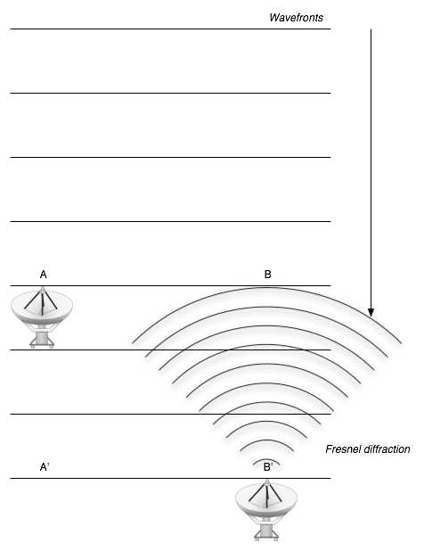
Figure 1: Diffraction of electric field on propagation from plane AB to plane A’B’. The correlation between the electric fields at point A and B is a two-dimensional Fourier transform of the sky brightness. Radiation at B is diffracted on propagation to plane A’B’, and so the measured correlation is no longer a Fourier transform of the sky brightness. Alternatively, in transmission, the electric field transmitted at B’ undergoes the Fresnel diffraction on propagation to the AB plane and so the correlation structure of the emitted radiation is altered. By the reciprocity theorem, these two descriptions are physically equivalent.

In figure (2), we show schematically the effect of this diffractive projection in $(u,v,w)$ space. A sample taken at $(u,v,w)$ is spread by diffraction over the $(u,v,w=0)$ plane. This may be interpreted as the sensitivity of a single sample point at non zero $w$ to a range of spatial frequencies across the field of view. From the sampling perspective, the effective diameter of the antennas in an interferometer is roughly the size of the Fresnel zone $r_{F}$. This can be very large - for the A configuration of the VLA at 74 MHz, this is about $r_{F}\sim 350m$.

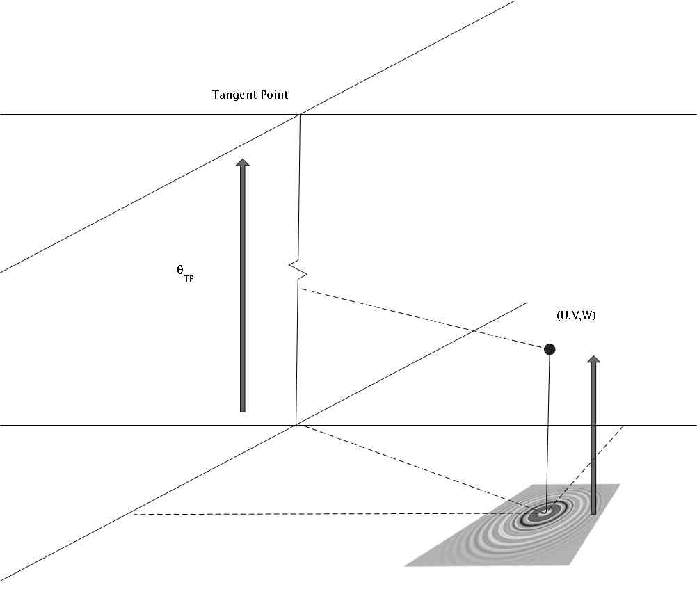
Figure 2: Schematic of the projection of a single $(u,v,w)$ sample onto the $(u,v,w=0)$ plane.

In summary, interferometers with the same $(u,v)$ but different $w$ provide substantially different information on the sky brightness. Hence, an interferometer can only be said to measure a single Fourier component of the sky brightness if $w=0$. For non-zero $w$, an interferometer is not a device for measuring a single Fourier component. In principle, then, by measuring at a fixed $(u,v)$ for a range of values of $w$, one can recover information on Fourier components within $r_{F}/\lambda$ of the nominal Fourier component sampling $(u,v)$. This is similar to the principle in mosaicing [Cornwell 1988] where by changing the pointing direction of the antennas in an interferometer, one can recover Fourier components within $D/\lambda$ of the nominal. However, in this case, one does not easily have access to samples spread along the w axis and so w-synthesis is less useful than mosaicing.

V Practical details of an algorithm for W-projection

V-A General structure

Given a model of the sky brightness, we can predict the visibility on the $(u,v,w=0)$ plane by a two-dimensional Fourier transform in $(\ell,m)$. Using the convolution function project this from the $(u,v,w=0)$ plane to any specific point $(u,v,w)$. The calculation in this direction (image to uvw-space) is limited only by numerical errors. Going in the opposite direction (uvw-space to an image) is more difficult. There is no inverse transform and so we have to rely upon iterative algorithms. As shown in Appendix A, we need to be able to apply the transpose of the image to uvw-space operation. In detail, this proceeds as follows: we project each $(u,v,w)$ point onto the $(u,v,w=0)$ plane using the W-projection function. We then Fourier transform (using a two-dimensional transform) these gridded visibilities to the image plane, where we have thus obtained a dirty (or residual) image on the tangent plane. The dirty image itself can be a good estimate of the sky brightness, depending upon the sidelobe level of the synthesized beam. More usually, though, deconvolution will be required. In this situation, the residual image may be used in a minor cycle deconvolution algorithm to update the model.

In the minor cycle, we use a single PSF calculated for the center of the field. This introduces errors comparable to the typical sidelobes so we terminate the minor cycle before these errors become significant.

V-B Aliasing

To limit aliasing, one must apply an additional tapering function in the image plane. The effective convolution function then becomes the Fourier transform of:

$$G_{T}(\ell,m,w)=T(\ell,m)e^{-2\pi i[w(\sqrt{1-\ell^{2}-m^{2}}-1)]}$$ (17)

Therefore to evaluate the visibility predicted for a pixellated model $I$ of the sky brightness, we do the following:

1. Multiply the sky brightness model $I$ by the taper function $T$.

2. Perform two dimensional Fourier transform (real to complex) of the tapered $T.I$.

3. Evaluate the convolution (equation 12) for each sample point to obtain the predicted visibility.

To evaluate the dirty (non-deconvolved) image:

1. For each sample visibility, evaluate the convolution for a gridded $(u,v,w=0)$ plane.

2. Perform two dimensional inverse Fourier transform (complex to real) to obtain the tapered $T.I^{D}$ (where $I^{D}$ denotes the dirty image).

3. Divide out the image plane tapering function $T$ to obtain the dirty image.

Numerical integration is required to find $\tilde{G_{T}}$. We use 4x padding in the image plane, equal spacing of $\sqrt{w}$ planes, and truncation of the aggregate convolution function (at 0.1%). These values have been determined empirically from the requirement that aliasing is suppressed at a dynamic range of $10^{4}$ or better. For better performance, it will be worthwhile to design a 2D FIR filter to approximate $\tilde{G_{T}}$ more exactly.

In figure (3), we show the image plane function and Fourier transform for $w=0,w_{max}/2,w_{max}$ for a typical observation with the VLA. For $w=0$, the convolution function is simply the usual spheroidal function. For $w$ increasing, the area of the $(u,v)$ plane affected by the projection of any point increases approximately as $\sqrt{w}$.

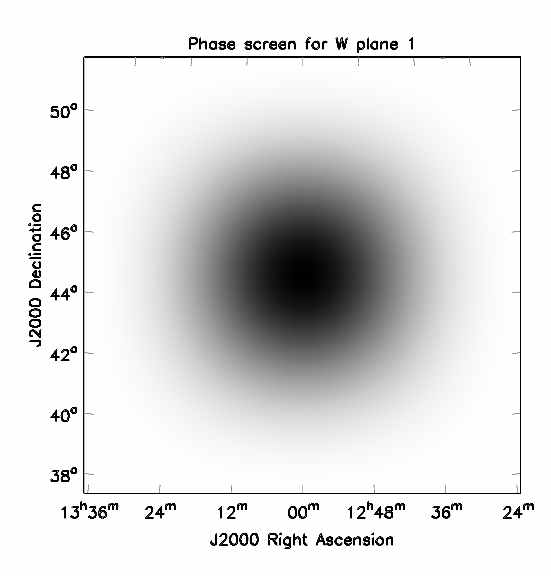
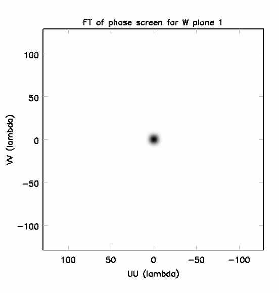
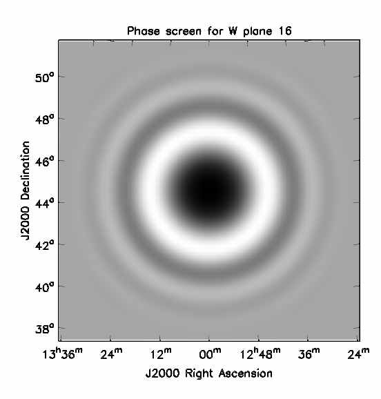
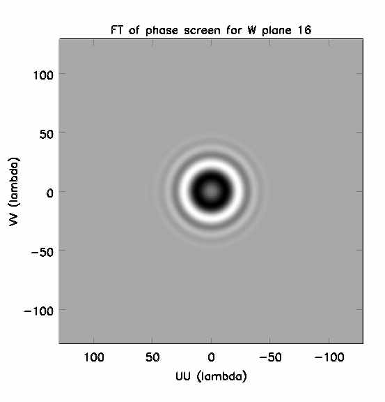
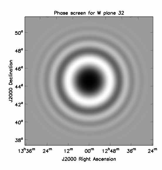
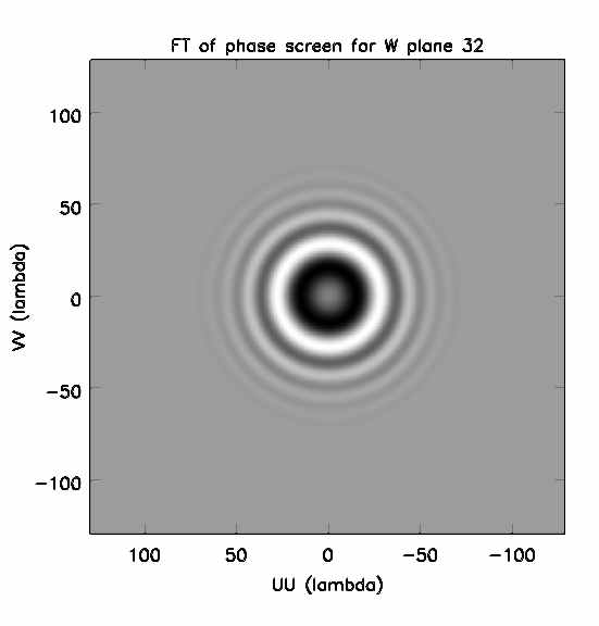
Figure 3: Image plane function and Fourier transform for (top) $w=0$, (middle) $w=w_{max}/2$, (bottom) $w=w_{max}$. The range of brightness is -1 to +1.

For the image plane tapering function $T$, we use a spheroidal gridding function. The usual spheroidal gridding function has support 9 by 9 pixels in $(u,v)$. The support of $\tilde{G_{T}}$ grows with both $w$ and the field of view, typically up to a largest value of about 70 by 70. The maximum memory required per plane is a few MB, for a total of up to 1GB - an amount which is common in desktop computers only in the last few years. The work involved in convolving with this function increases in direct proportion to the extent in $(u,v)$. The average value of $|w|$ gridded is close to $w_{max}/2$, so the typical increase in gridding costs is about a factor of 10-20. While increasing the spread of $\tilde{G_{T}}$ in $(u,v)$ directly leads to more computing, the extra cost incurred by using more planes in $w$ is relatively minor - all that happens is an essentially negligible increase in the memory access time required to get the relevant part of the convolution function.

Tabulation of $\tilde{G_{T}}$ in $w$ leads to aliases at the scale size of $1/\Delta w$. Placing these aliases outside the field of view requires that $w$ be sampled with similar precision to $(u,v)$. Tabulating planes evenly in $\sqrt{w}$ reduces this effect to a tolerable level. With this in place, the remaining errors are due to the incorrect value of the convolution function being used. Since this aliasing error is localized in $\sqrt{w}$, the resulting error is not coherent in the image plane. This is in contrast to the facet approaches where the prediction error is necessarily worse on the longest baselines, and so the resulting error patterns are quite coherent in the image.

V-C Computational load

Most of the computational load lies in the gridding/degridding step which is directly determined by the number of visibility samples and the size of the convolution kernel. Taking the field of view to be $\lambda/D$, we find that the number of pixels needed in the convolution kernel along each of the $u$ and $v$ axes goes as $B\lambda/D^{2}$.

The costs for facet based gridding go as the total number of facets (i.e. the product of the number along each of the two spatial axes). We then have that the costs per sample go as:

$$t_{facets} = N^{2}_{facets}.N^{2}_{GCFpoints}.t_{single}$$ (18)

$$t_{wproject} = 2(N^{2}_{wproject}+N^{2}_{GCFpoints}).t_{single}$$ (19)

In this equation, $N_{GCFpoints}$ is the support of the normal gridding convolution function in one axis (typically 9), and $t_{single}$ is the time to grid a single sample to a single grid point. $N_{facets}$ (the number of facets in one axis) and $N_{wproject}$ (the typical size of the $\tilde{G_{T}}$ gridding function) are both proportional to $B/(\lambda D^{2})$ but with different proportionality constants. We have assumed that the sizes of the normal gridding convolution function and $\tilde{G}$ add in quadrature. Note also that $\tilde{G_{T}}$ is necessarily complex. If we take $N_{facets}$ and $N_{wproject}$ to be roughly equal, then for large fields of view, the ratio of these times is roughly the total number of points in the normal gridding convolution function. Since the normal gridding convolution function is typically 7 by 7 or 9 by 9, the asymptotic speedup is between 25 and 50. Allowing for different proportionality constants, we could conservatively expect at least an order of magnitude speed advantage for W-projection. The gains for less severe non-coplanarity will be smaller. In the next section, we examine the relative performance for simulated data.

At first sight, it is curious that W-projection should be faster than the facet approaches. However, we can see from the analysis just given that the discrepancy comes from the relative inefficiency of using a broad convolution function in the standard FT approach. If box-car convolution were to be used in facet based imaging, the computing costs would be roughly the same for the two approaches.

V-D Implementation

We have implemented the various algorithms (standard FT, uvw-facets, and W-projection) in AIPS++/CASA. Most of the code is C++ using AIPS++/CASA libraries, but inner loops for gridding and Fourier transformation are written in hand-optimized Fortran. Possible minor cycle deconvolution steps being standard CLEAN, a multi-scale CLEAN algorithm [BhatnagarCornwell2004 ], or a Maximum Entropy algorithm [Cornwell & Evans 1985].

VI Simulated data

Non-isoplanatism is most troublesome for fields full of emission, and the non-coplanar baselines effect is greater for longer wavelengths. Accordingly, we simulated a low frequency observation of a typically full field: a 74MHz VLA C-configuration full synthesis on a field at right ascension 12h56m57.18, declination 47d20m20.801. The data consisted of 505440 visibility records, each of 8 spectral channels. The sources were generated by taking the sixty six Westerbork Northern Sky Survey (WENSS) [Rengelink et al. 1997] sources brighter than 2Jy within 12 degrees of the specified center. The sources were scaled to 74MHz by a spectral index of -0.7, and then multiplied by a simple model of the 74MHz antenna primary beam. The data corresponding to these scaled sources were calculated using analytical transforms, and should thus be fully accurate to machine precision. The brightest source has strength 47.8Jy and has been chosen to be at the field center. The data generated is somewhat realistic for a randomly chosen 74MHz field observed with the VLA, the major deficiency being the lack of weak sources.

The processing was performed on a dual Xeon 3.06GHz machine with per-processor cache 512k and 3GB of memory. AIPS++ was compiled using the GNU suite of compilers with optimization flags set to O2.

For this type of confused field observed with the VLA, deconvolution is necessary. All images were cleaned with 20,000 iterations at a loop gain of 0.1. Both uvw-space facet and W-projection algorithms used in-memory gridding and Fourier transform. The image size was 1536 by 1536 pixels of 60arcsec. The maximum support of the gridding function $\tilde{G_{T}}$ is 220 pixels (full width). We use a gridding function of size 512 by 512 complex pixels for each plane so the memory required for storage of the gridding function is 2MB per plane.

The results are shown in Table I and displayed in Figure 4. The key points are:

• For the specific case tested here, W-projection is about 20 times slower than standard two dimensional Fourier transformation. We may understand this as follows: The standard gridding uses support of 9 by 9 pixels. The typical size of the convolution region in W-projection is about 30 by 30 pixels so the increased load in gridding for W-projection should be about (2*30*30/9*9) times bigger or a factor of 24. This rough agreement indicates that the W-projection costs are in proportion to the increase in multiplications in the innermost loop.

• For the same dynamic range, W-projection is about an order of magnitude faster than uvw-space facets.

• For W-projection, the aliasing performance and initialization time both grow linearly with the number of planes, whereas the residual calculation time is independent of the number of planes (in fact a slight decrease is seen as the number of planes increases).

• For uvw-space facets, the aliasing performance and the residual calculation times both grow linearly with the number of facets (i.e. the inverse square of Fresnel number).

TABLE I: Table I: Performance of various methods on simulated 74MHz C configuration observations. The first column shows the approach used, the second is a robust estimate of the dynamic range after cleaning (DR1=peak/(median absolute deviation from the median)), the third is the dynamic range on a bright source (DR2=peak/abs(max near negative)), the fourth is the time in seconds to initialize the convolution functions, the fifth is the time taken to calculate the residual image (involving a transform in both directions), and the last is the total time to deconvolve.

Method	DR1	DR2	Calc G	Calc res	Total
FT	1570	2.8	-	27	216
uvw-facets (3 by 3)	2550	3.6	-	204	784
uvw-facets (9 by 9)	12580	40	-	1348	30488
w-proj (8)	2692	17	9	671	2748
w-proj (16)	4665	53	18	661	2688
w-proj (32)	9066	268	35	647	3985
w-proj (64)	18198	524	83	607	3161
w-proj (128)	33370	856	103	532	3857
w-proj (256)	50888	984	231	507	5419

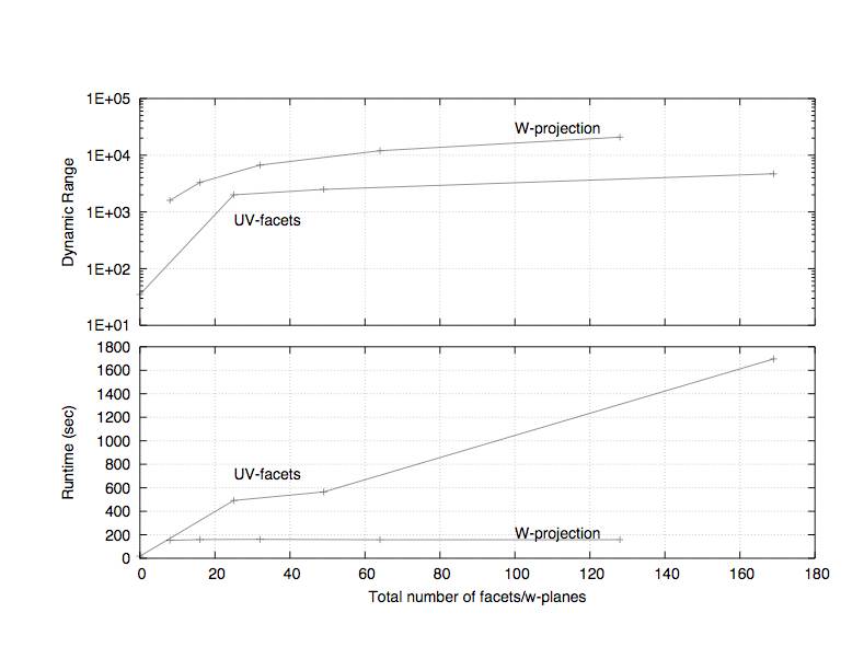
Figure 4: Performance of the two methods: uv-facets and W-projection. Lower panel shows the actual runtime (smaller is better) as a function of total number of uv-facets $N^{2}_{facets}$ for the uv-facets algorithm and as a function of total number of w-planes for the W-projection algorithm. Top panel shows the achieved dynamic range (larger is better) in the simulations as a function of the number of uv-facets/w-planes. For a given number of facets/w-planes, the runtime and the dynamic range both are in favour of W-projection algorithm.

In figure (5), we compare the restored images obtained from standard FT, uvw-space facets (9 by 9), and W-projection (256). A few comments:

• The standard FT image shows severe distortion of sources away from the phase center. For the uvw-facets approach, the distortion is reduced but is still present for sources away from a facet center (as shown by DR2).

• The errors in W-projection image are much more isotropic (as evidenced by comparison of the DR1 and DR2 numbers).

• The computing time differential between uvw-facets and W-projection in residual calculation is about a factor of thirty, and the error performance about 3, both in favor of W-projection.

• The uvw facets algorithm has a relative advantage early in iteration because it need not Fourier transform (to the visibility plane) any facets empty of emission. This partially accounts for the difference between the factor of thirty for residual calculation and six overall. In addition, the scaling of the Clean minor cycle slightly favors the uvw facets algorithm.

• Extrapolating the uvw-space facets behavior, we find that to obtain the same dynamic range as the best W-projection image, about 27 by 27 facets would be required, at a cost of about 100 compared to w projection.

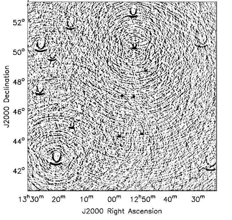
(a) standard Fourier transform

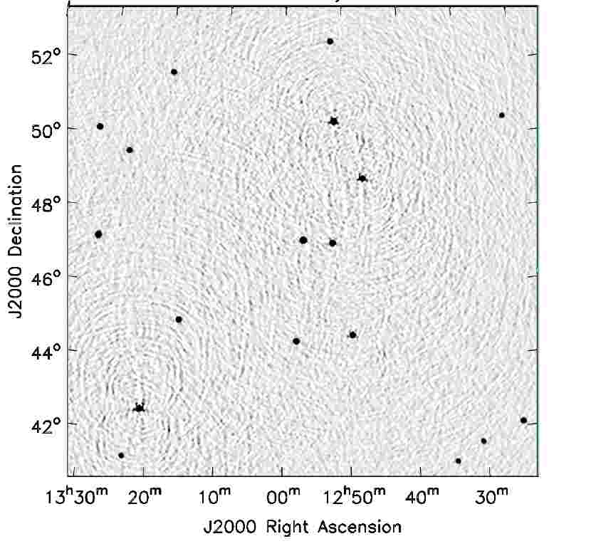
(b) uvw-space facets (9 x 9)

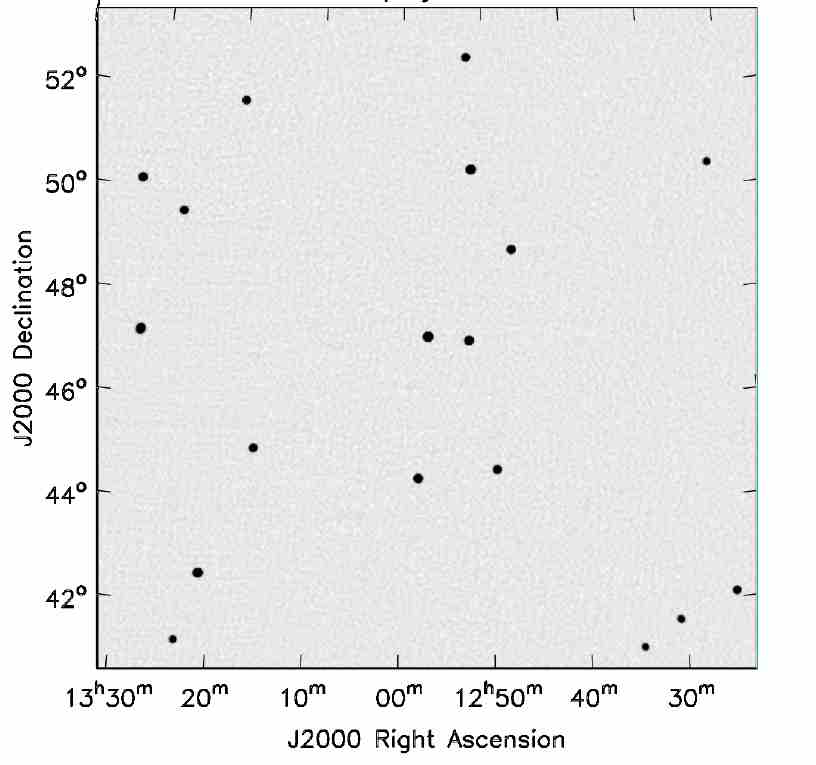
(c) W-projection (128 ${\tilde{G}_{T}}$ planes)

Figure 5: Clean images for 74MHz simulation. The brightness range is -5 to +50 mJy/beam, and the peak brightness should be 47.2Jy. The peak sidelobes around the brightest sources in the uvw-space facets image are about 0.3%. Calculation of these images took 784s, 30488s, and 5419s respectively.

VII A wide-field image of the SN1006 at 1.4GHz

As an example of the application of W-projection to real data, we show an image of the supernova remnant SN1006 observed at 1.4GHz. The data are from all the four configurations of the Very Large Array (VLA) and Green Bank Telescope (GBT). Details of the data reduction and scientific interpretation are given elsewhere Dyer [2005]. The GBT image was deconvolved using a Maximum Entropy algorithm, and this image was then used as a starting point for a multi-scale CLEAN algorithm BhatnagarCornwell2004 . Our W-projection approach was used for the major cycle of the CLEAN algorithm. An image plane facet based algorithm would require at least 10 by 10 facets, thus crisscrossing the extended emission. For W-projection, we used 256 planes.

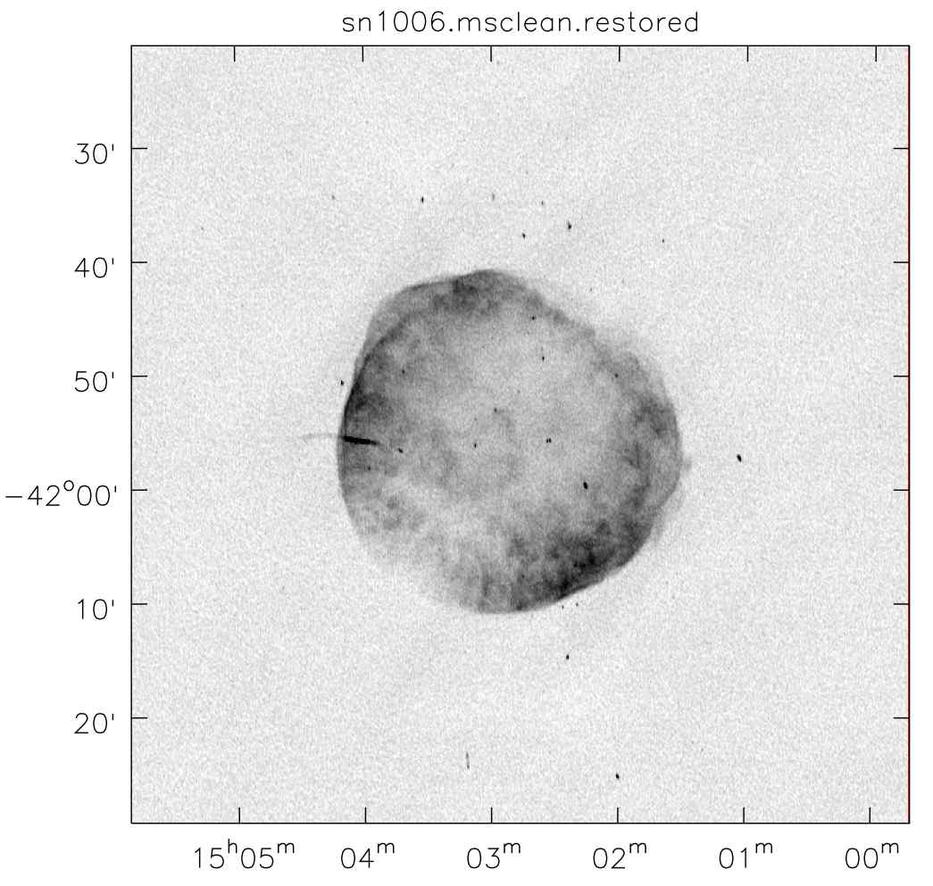
Figure 6: Multi-scale CLEAN image of the SN1006 made using W-projection (256 planes) and a multi-scale CLEAN algorithm. A facet-based algorithm would have required approximately 10 by 10 facets.

VIII Implications

The results in this paper have a number of implications for the design and operation of wide-field imaging radio synthesis telescopes.

First, the meaning of redundancy in wide-field imaging is much more restrictive than often thought. To get the same visibility, one must measure at exactly the same $(u,v,w)$ - having identical $(u,v)$ is not adequate. This means that redundant self-calibration or data-editing is limited in applicability for wide-field imaging.

Second, calculating images for wide field of view will be less demanding than expected. Our algorithm is substantially faster, and scales much more slowly with desired precision than the facet based algorithms. As shown in the simulations, the precision of the facet approaches scales roughly as the square root of the computational time, whereas that for W-projection is roughly independent of the computational time, the cost mainly being in memory.

Perley & Clark [2003] derived scaling relationships for the computing costs associated with wide-field imaging as a function of antenna diameter and baseline length. They based their analysis on faceted algorithms. As shown above, the computational costs of W-projection can be less by about an order of magnitude. This affects only the coefficients in the Perley-Clark cost equation, not the form. However, an order of magnitude is a very substantial gain, equivalent to about 5 years of Moore’s Law growth. Cornwell [2004] has evaluated computing costs for the Square Kilometer Array and Expanded Very Large Array in light of the W-projection algorithm.

The cost of convolution with $\tilde{G_{T}}$ can get to be quite large. We show representative values for the size of $\tilde{G_{T}}$ in Table II. The very large values found for few hundred kilometer baselines at meter wavelengths may require another shift in algorithm design, perhaps to a hybrid W-projection/uvw facets approach. Whether this is so depends upon the architecture of the machines on which such processing will be performed. It is clear that the memory requirements currently prohibit W-projection on a single processor computer for the very worst cases, unless some symmetry properties are exploited.

TABLE II: Table II: Support of $\tilde{G_{T}}$ (half-width in pixels) as a function of maximum baseline length and wavelength. These have been scaled from values found in the simulation described above. For the diameter of the VLA antennas, 25m, these numbers are within a few percent of the Fresnel radius $r_{F}$ in meters.

Wavelength		4m	1m	0.2m	0.06m
Baseline (m)	Image size
1000	240	58	29	13	7
3500	840	109	54	25	13
10000	2400	184	92	42	23
35000	8400	344	172	79	42
100000	24000	582	291	133	71
350000	84000	1089	544	249	133

This naturally brings up the question of how best to parallelize the W-projection algorithm. Parallelization of the image- and uvw space-facets algorithms has been demonstrated [Cornwell 1993; Golap et al. 2001]. The facet-based algorithms are parallelized by delegating the residual calculation for each facet to a separate processor. Each processor must access every record of a visibility data set and communicate back the cleaned residual image for a single facet. Golap et al. [Golap et al. 2001] demonstrated reasonable scaling for imaging of 15 by 15 facets for up to 32 processors, linear up to 16 and flattening slightly at 32. This flattening is thought to be due to I/O blocking, and so parallel I/O may be necessary. For W-projection, the natural partitions are the separate planes in $\sqrt{w}$. In this scenario, the gridding for each $\sqrt{w}$ plane is delegated to a separate processor which need only store the visibility data for that plane and at the end of gridding, the separate image grids are simply added, either before or after Fourier transform. This has the side-benefit of reducing the memory cost per processor to an affordable level. Each processor has to read only a small sub-set of the records in a visibility data set, and must communicate back a copy of the entire residual image. Parallelization of the minor-cycle deconvolution depends on the algorithm used.

IX Summary

We have demonstrated a new algorithm for correcting the non-coplanar baselines effect. This has superior performance in both speed and error control, at the cost of greater memory usage. These advantages grow more substantial as the non-coplanarity grows more severe. It does not make it necessary to use only pixel based conventional CLEAN deconvolution step and thus is well-suited to wide-field imaging of very extended emission (for example, the Galactic plane) where multi-scale or Maximum Entropy methods are required.

The facets algorithms remain roughly competitive with W-projection only at low dynamic range, for example that occuring in VLA observations at 74MHz. At high sensitivities, W-projection will be decisively superior. Hence use of this algorithm (and similar algorithms for other problems) will have a substantial impact on the predicted computing costs for new radio synthesis arrays such as the EVLA, LOFAR, and SKA.

Appendix A: General structure of imaging algorithms

The scientific impact of radio interferometry has been heavily influenced by the advent of deconvolution and self-calibration algorithms, starting with Clean in the mid-seventies [see Thompson et al. 2001]. The introduction of the minor/major cycle approach (such as the Clark CLEAN algorithm and the Cotton-Schwab CLEAN) has aided the generation of new deconvolution algorithms. In such algorithms, the deconvolution is split into two cycles, the minor cycle using an approximate PSF for computational speed, and the major cycle using a full calculation for accuracy. Much of imaging then reduces to two steps:

• Finding and solving an approximate convolution problem for the minor cycle.

• Performing the major cycle with computational efficiency and high numerical accuracy.

First, we should clarify a few definitions. Nearly all of the pure imaging problems are linear in the pixel values (unlike the calibration problem, which is non-linear in the unknown antenna gains). We can therefore write a linear equation:

$$D=AI+N$$ (20)

where $D$, $I$ and $N$ are vectors for data, image, and noise, and $A$ is the (non-square) observation matrix. In the usual case of simple radio interferometry, the elements of $A$ are the cosines and sines of the Fourier transform. The observation matrix is then usually singular and cannot be simply inverted. Instead, it is generally the case that non-linear iterative methods are used to solve this linear equation.

The normal equations arising from least squares minimization of the image pixels are:

$$A^{T}D=A^{T}AI$$ (21)

For the simple case where $A$ represents a Fourier transform (or discrete sum), $A^{T}D$ is the dirty image, and $A^{T}AI$ is the true sky $I$ convolved with the dirty beam $A^{T}A$. (Note that we have left out the covariance matrix of the noise for simplicity, though in practice, this must be taken into account).

Interpreting the deficit as a residual image, we have:

$$I^{R}=A^{T}(D-AI)$$ (22)

Calculating $I^{R}$ for a given model image $I$ constitutes the major cycle. This consists of two steps - first the calculation of the residual data $D-AI$, and second the calculation of the residual image $A^{T}(D-AI)$. The first step must be done with high accuracy but the second need only be done approximately. Let $B$ be an approximation to $A^{T}$; we then find it convenient to work with the approximate residual image:

$$I^{AR}=B(D-AI)$$ (23)

The minor cycle consists of finding an update to the image $I$ given either the residual image $I^{R}$ or the approximation $I^{AR}$. In some circumstances, the minor cycle need not be done with high accuracy because any errors will be corrected in the major cycle. Since most of our most efficient algorithms are for shift-invariant PSFs, it pays to try to find an approximate shift-invariant convolution to be solved in the inner loop. For example, for a homogeneous mosaic, the linear mosaic of the individual dirty (residual) images can be approximated as a convolution of the true image with an approximate PSF [Cornwell et al. 1993]. As another example, the nominally shift-variant PSF encountered in the non-coplanar baselines effect can be often be approximated by a shift-invariant PSF for the minor cycle.

The computational costs of deconvolution thus split into two parts:

• Calculating the normal equations: specifically the predicted data $AI$, and the residual image $A^{T}(D-AI)$.

• Updating the model using the residual image $A^{T}(D-AI)$.

References

- [1] Bhatnagar, S. & Cornwell, T., Scale Sensitive Deconvolution of Interferometric Images, 2004, Astron. & Astrophys., 426, 747-754
- Bracewell [1983] Bracewell, R. 1983, Inversion of Non-Planar Visibilities. In Measurement and Processing for Indirect Imaging. Proceedings of an International Symposium held in Sydney, Australia, August 30-September 2, 1983. Editor, J.A. Roberts; Publisher, Cambridge University Press, Cambridge, England, New York, NY, 1984. P.177
- Brouw [1969] Brouw, W. 1969, Data Processing for the Westerbork Synthesis Radio Telescope (Ph.D. thesis, Univ. of Leiden)
- Clark [1980] Clark, B., An efficient implementation of the algorithm ’CLEAN’, 1980, Astron. & Astrophys., 89, 377
- Clark [1980] Clark, B., Curvature of the Sky, 1973, VLA Scientific Memo 107 (National Radio Astronomy Observatory, http://www.nrao.edu)
- Cornwell [1988] Cornwell, T., Radio-interferometric imaging of very large objects, 1988, Astron. & Astrophys., 202, 316
- Cornwell [1993] Cornwell, T., Improvements in Wide-Field Imaging, 1993, VLA Scientific Memo 164 (National Radio Astronomy Observatory, http://www.nrao.edu)
- Cornwell [2004] Cornwell, T., Ska and Evla Computing Costs for Wide Field Imaging, 2004, Experimental Astronomy 17:11, 329-343, 6/2004
- Cornwell & Evans [1985] Cornwell, T. & Evans, K., A simple maximum entropy deconvolution algorithm 1985, Astron. & Astrophys., 143, 77
- Cornwell et al. [1995] Cornwell, T., Briggs, D., & Holdaway, M. 1995, User Guide to SDE (NRAO, Socorro)
- Cornwell et al. [1993] Cornwell, T., Holdaway, M., & Uson, J., Radio-interferometric imaging of very large objects: implications for array design, 1993, Astron. & Astrophys., 271, 697
- Cornwell & Perley [1992] Cornwell, T. & Perley, R., Radio-interferometric imaging of very large fields - The problem of non-coplanar arrays, 1992, Astron. & Astrophys., 261, 353
- Dyer [2005] Dyer, K., et al., High-resolution Flux-accurate Radio Images of SN1006, 2005, Bulletin of the American Astronomical Society, Vol. 37, p.1437
- Ekers [2003] Ekers, R., Square Kilometre Array (SKA), 2003, in ASP Conf. Ser. 295: Astronomical Data Analysis Software and Systems XII, 125–+
- Frater & Docherty [1980] Frater, R. & Docherty, I., On the reduction of three dimensional interferometer measurements, 1980, Astron. & Astrophys., 84, 75
- Golap et al. [2001] Golap, K., Kemball, A., Cornwell, T., & Young, W., Parallelization of Widefield Imaging in AIPS++, 2001, in ASP Conf. Ser. 238: Astronomical Data Analysis Software and Systems X, 408
- Goodman [2002] Goodman, J. 2002, Introduction to Fourier Optics (McGraw Hill)
- Perley [2000] Perley, R., The Very Large Array Expansion Project, 2000, in Proc. SPIE Vol. 4015, p. 2-7, Radio Telescopes, Harvey R. Butcher; Ed., 2–7
- Perley & Clark [2003] Perley, R. & Clark, B., Scaling Relations for Interferometric Post-Processing, 2003, EVLA memo 63 (National Radio Astronomy Observatory, http://www.nrao.edu)
- Sault et al. [1999] Sault, R., Bock, D.-J., & Duncan, A., Polarimetric imaging of large fields in radio astronomy, 1999, Astron. & Astrophys., 139, 387
- Taylor et al. [1999] Taylor, G., Carilli, C., & Perley, R., eds. 1999, Synthesis Imaging in Radio Astronomy II
- Perley et al. [1989] Perley, R., Schwab, F. R., & Bridle, A.H., eds. 1999, Synthesis Imaging in Radio Astronomy
- Thompson et al. [2001] Thompson, A., Moran, J., & Swenson, G. 2001, Interferometry and synthesis in radio astronomy (Wiley, New York)
- Rengelink et al. [1997] Rengelink, R. B., Tang, Y., de Bruyn, A. G., Miley, G. K, Bremer, M. N., Rottgering, H. J. A. & Bremer, M. A. R.,The Westerbork Northern Sky Survey (WENSS), 1997, Astron. Astrophys. Suppl., 124, 259-280
Acknowledgement
We thank the AIPS++/CASA Project team for providing a superb software environment in which to do this development, resulting in the happy situation where most of the time in this project went to thinking and experimentation rather than the coding. TJC thanks Wim Brouw for his patience in explaining simple geometry via email, and David King for many stimulating and insightful questions. We all thank the Fridays-on-Thursdays group in Socorro for many hours of conversation relevant to imaging. Kristy Dyer kindly allowed us to use her SN1006 data.