Commutative limit of a renormalizable noncommutative model

Abstract

Renormalizable $\phi^{\star 4}_{4}$ models on Moyal space have been obtained by modifying the commutative propagator. But these models have a divergent “naive” commutative limit. We explain here how to obtain a coherent such commutative limit for a recently proposed translation-invariant model. The mechanism relies on the analysis of the uv/ir mixing in Feynman graphs at any order in perturbation theory.

Keywords: noncommutative quantum field theory, Moyal space, commutative limit

1 Introduction

Noncommutative field theory [1] is a subject which lies at the intersection of many different perspectives. It is a natural generalization of Alain Connes noncommutative geometry program [2], it is an effective regime of string theory [3, 4], and of loop quantum gravity [5]. It has also the potential to throw light on difficult non perturbative physical problems (quantum Hall effect [6, 7, 8], quark confinement…). For a recent review, see [9].

The issue of renormalization of noncommutative (Euclidean) field theory on Moyal space however was made difficult by the discovery of ultraviolet/infrared mixing [10]. In the simple case of the $\phi^{\star 4}_{4}$ model a first solution was obtained by H. Grosse and R. Wulkenhaar, who modified the ordinary propagator, adding a harmonic potential term [11]. The resulting theory has a new symmetry called Langmann-Szabo or LS duality [12]. This result has sparked a flurry of activity. The corresponding ”GW” model (and other related models) have been shown fully renormalizable by all the main methods; furthermore, different field theoretical properties have been exbited [13, 14, 15, 16, 17, 18, 19, 20]. Even more important, it is the first example of a non supersymmetric field theory in four dimensions which has a non trivial ultraviolet fixed point [21, 22, 23]. It is currently under construction in a non perturbative sense [24, 25], something which has never been fully done for any four dimensional commutative theory. Noncommutative gauge theories with some version of LS symmetry are actively searched for [26, 27, 28]. However in spite of this great conceptual and mathematical interest the GW model has for the moment no direct phenomenological applications. It breaks translation invariance and it seems very difficult to connect it continuously to ordinary field theory at lower energy. In technical terms the $\theta\to 0$ limit of the GW model seems too singular.

These drawbacks motivated the introduction in [29] of another $\phi^{\star 4}_{4}$ model which is translation invariant and also renormalizable to all orders in perturbation theory. It is not based on the LS symmetry, hence it may not be fully constructible in a non perturbative sense. However it may be easier to connect to ordinary high energy physics. To support this idea comes the recent proof [30] that the $\beta$ function of this model is just a rational multiple of the commutative model $\beta$ function. Let us emphasize here that this result, in spite of the title of [30], was proven there at any order in perturbation theory.

Let us further state here that the parametric representation for this model was obtained in [31]. Also some one-loop and higher order Feynman amplitudes were explicitly computed in [32]. Furthermore, the static potential associated to this noncommutative model was calculated in [33]. Moreover, the idea of the translation-invariant scalar model proposed in [29] was also extended to the level of noncommutative gauge fields [34]. For a review of this developments, the interested reader may report himself to [35].

In this paper we study how in this model the $1/p^{2}$ counterterms created by the uv/ir mixing graphs can morph into the ordinary mass and wave function counterterms that these graphs generate in the ordinary commutative $\phi^{4}_{4}$ as the $\theta$ parameter is turned off. In this way we show how a renormalizable noncommutative model can become an effective commutative model. This is a small step in the direction of smoothing the road between commutative and noncommutative field theory. Note that such a mechanism could also give insights on the noncommutative limit of the gauge models [34]. Commutative field theory certainly works well at least up to the LHC energies, but a noncommutative field theory regime might be relevant somewhere between the LHC scale and the Planck scale where gravity has to be quantized.

2 Scalar field theory on the Moyal space

In this section we recall the definition of the noncommutative Moyal space on which we consider scalar quantum field theory. Furthermore, some general considerations which respect to the associated Feynman graphs are given.

2.1 The “naive” $\phi^{\star 4}$ model

This model is obtained by replacing in the ordinary $\phi^{4}$ action the pointlike product by the Moyal-Weyl $\star$-product

$$S[\phi]=\int d^{4}x\Big{(}\frac{1}{2}\partial_{\mu}\phi\star\partial_{\mu}\phi+\frac{1}{2}m^{2}\phi\star\phi+\frac{\lambda}{4!}\phi\star\phi\star\phi\star\phi\Big{)}(x),$$ (2.1)

with Euclidean metric. The commutator of two coordinates is

$$[x_{\mu},x_{\nu}]_{\star}=i\Theta_{\mu\nu},$$ (2.2)

where

$$\Theta=\begin{pmatrix}0&\theta&0&0\\ -\theta&0&0&0\\ 0&0&0&\theta\\ 0&0&-\theta&0\end{pmatrix},$$ (2.3)

and $\theta$ is the noncommutativity parameter. In momentum space, the action (2.1) becomes

$$S(\phi)=\frac{1}{(2\pi)^{4}}\int d^{4}p\Big{(}\frac{1}{2}p^{2}\phi(-p)\phi(p)+\frac{1}{2}m^{2}\phi(-p)\phi(p)+\frac{\lambda}{4!}V_{\theta}(\phi,p)\Big{)},$$ (2.4)

where the interaction potential is:

$$V_{\theta}(\phi,p)=\frac{1}{(2\pi)^{8}}\int d^{4}qd^{4}k\ \hat{\phi}(p)\hat{\phi}(q)\hat{\phi}(k)\hat{\phi}(-p-q-k)e^{-\frac{i}{2}(p\wedge q+p\wedge k+q\wedge k)}.$$ (2.5)

Note that we have used the notation:

$$p\wedge q=p_{\mu}\Theta^{\mu\nu}q_{\nu}.$$

2.2 Feynman graphs: planarity and non-planarity, rosettes

In this subsection we give some useful conventions and definitions. Consider a $\phi^{\star 4}$ connected graph with $n$ vertices, $L$ internal lines and $F$ faces. One has

$$2-2g=n-L+F,$$ (2.1)

where $g\in{\mathbb{N}}$ is the genus of the graph. If $g=0$ the graph is planar, if $g>0$ it is non-planar. Furthermore, we call $B$ the number of faces broken by external lines, and we say that a planar graph is regular if $B=1$.

The $\phi^{4}$ graphs also obey the relation

$$L=2n-N/2,$$ (2.2)

where $N$ is the number of external legs of the graph.

In [36], several contractions or ”Filk moves” were defined on a Feynman graph. The first Filk move, which is the one we use in the sequel, consists in reducing a tree line by gluing up together two vertices into a bigger one.

Repeating this operation for the $n-1$ lines of a spanning tree, one obtains a single final vertex with all the loop lines hooked to it - a rosette (see Fig. 1).

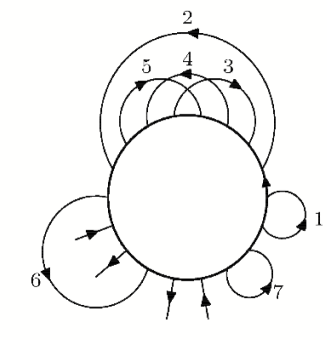
Figure 1: An example of a rosette

Note that the number of faces or the genus of the graph do not change under this operation. Furthermore, the external legs will break the same faces on the rosette. When one deals with a planar graph, there will be no crossing between the loop lines on the rosette. The example of Fig. 1 corresponds thus to a non-planar graph (one has crossings between the loop lines $3$, $4$ and $5$).

In [36] the general oscillating factors appearing in the Feynman integrand as a function of the corresponding rosette were computed. We do not recall here these results, but will use some particular cases when necessary.

3 Uv/ir mixing as insight for the commutative limit

The uv/ir mixing comes from the 2-point planar irregular graphs. We will first recall the analysis of the “non-planar” tadpole and then extend it to any 2-point planar irregular Feynman graph.

3.1 The “non-planar” tadpole

The Feynman amplitude ${\cal A}_{G_{0}}$ of the “non-planar” tadpole $G_{0}$ of Fig. 2 writes, up to some constant factor

Figure 2: The “non-planar” tadpole graph.

$${\cal A}_{G_{0}}(k)=\int d^{4}p\,\frac{e^{ip\wedge k}}{p^{2}+m^{2}}.$$ (3.1)

The oscillating factor above is responsible for the convergence of the integral. One can thus interpret $\theta^{-\frac{1}{2}}$ as some kind of uv cut-off. Indeed, when $\theta=0$ the integral is no longer convergent and (3.1) will simply correspond to the divergent planar tadpole, leading to the usual mass renormalization. This observation comes from the fact that the amplitude (3.1) computes to

$$\begin{cases}\infty&\mathrm{if}~{}\theta=0,\\ \sqrt{\frac{m^{2}}{\theta^{2}k^{2}}}K_{1}(\sqrt{m^{2}\theta^{2}k^{2}})\approx_{|p|\to 0}\frac{1}{\theta^{2}k^{2}}&\mathrm{if}~{}\theta\neq 0,\\ \end{cases}$$ (3.2)

where again, in the second line above, we have omitted some inessential constants.

3.2 General 2-point planar irregular graphs

Let us now prove that in the case of a general 2-point planar irregular Feynman graph, the considerations of the previous subsection still hold.

As before, let us denote the external moment of a two-point graph by $k$. One has $B=2$. When shrinking the graph to a rosette (as described in section 2.2), one can always choose one of the external legs to break the ”external face”. The other external leg then breaks an internal face (see for example Fig. 3, where this internal face corresponds to line $p_{1}$).

Figure 3: An example of a rosette obtained from a two-point graph with $3$ internal lines.

The general amplitude contains an oscillating factor (see again [36] for further details)

$$e^{-ik\wedge(a^{j}p_{j})}.$$

The linear combination $a^{j}p_{j}$ corresponds to the sum of momenta of the lines arching over this second external leg, where the coefficients $a_{j}$ are $\pm 1$ . In the example of Fig. 3, because of the orientation of the lines one has to take the internal momenta $p_{1}$ and $p_{3}$ with opposite signs: $a^{j}p_{j}=p_{1}-p_{3}$. A general Feynman amplitude writes

$${\cal A}_{G}=K\int\prod_{i=1}^{L}d^{4}p_{i}\frac{e^{-ik\wedge(a^{j}p_{j})}}{\prod_{i=1}^{L}(p_{i}^{2}+m^{2})}.$$ (3.3)

As in the case of the non-planar tadpole, we express now the integral above in function of the Schwinger parameters $\alpha_{\ell}$ ($\ell=1,\ldots,L$). One can then check (see [31] for a more detailed analysis) that after performing the Gaussian integrals over the internal momenta $p_{i}$, one obtains an integral of the following type

$$\int_{0}^{\infty}U^{-2}(\alpha)e^{-m^{2}\sum_{j=1}^{L}\alpha_{j}^{2}}e^{-\frac{P(\alpha)}{U(\alpha)}k^{2}}.\exp(-\frac{k\circ k}{4\sum_{{\rm overarching}\ \ell}\alpha_{\ell}})$$ (3.4)

where

$$k\circ p=-k_{\mu}(\Theta^{2})^{\mu\nu}p_{\nu},\ (\Theta^{2})^{\mu\nu}=\Theta^{\mu\rho}\Theta_{\rho}^{\nu},$$ (3.5)

$U(\alpha)$ and $P(\alpha)k^{2}=V(\alpha,k)$ are the usual Symanzik (topological) polynomials of the ordinary commutative $\phi^{4}$ theory (since we deal with a two-point function there is a single external invariant $k^{2}$ in factor in $V$). The sum $\sum_{{\rm overarching}\ \ell}\alpha_{\ell}$ above denotes the sum on the parameters $\alpha$ associated to the tree lines (which were reduced to obtain the rosette) as well as on the parameters $\alpha$ associated to the lines overarching the internal broken face ($\alpha_{1}+\alpha_{3}$ in the example of Fig. 3). Note that

$$({\rm deg}\,U)^{2}=2(L-(n-1)).$$ (3.6)

Furthermore, since $L=2n-N/2$ and we deal with the two-point function ($N=2$) one has

$$({\rm deg}\,U)^{2}=2(L-(n-1))=L+1.$$ (3.7)

Let us recall that the polynomials $U$ and $V$ are explicitly positive.

Note that $\Theta^{2}=-\theta^{2}{\rm Id}$ so that integral (3.4) writes

$$\int_{0}^{\infty}U^{-2}(\alpha)e^{-m^{2}\sum_{j=1}^{L}\alpha_{j}^{2}}e^{-\frac{P(\alpha)}{U(\alpha)}k^{2}}\exp(-\frac{\theta^{2}k^{2}}{4\sum_{{\rm overarching}\ \ell}\alpha_{\ell}})\prod_{i=1}^{L}d\alpha_{i}.$$ (3.8)

In the uv regime ($\alpha_{\ell}\to 0$), one needs to consider only

$$\int_{0}^{\infty}U^{-2}(\alpha)e^{-m^{2}\sum_{j=1}^{L}\alpha_{j}^{2}}\exp(-\frac{\theta^{2}k^{2}}{4\sum_{{\rm overarching}\ \ell}\alpha_{\ell}})\prod_{i=1}^{L}d\alpha_{i}.$$ (3.9)

We now analyze this integral by performing the following change of variable:

$$\alpha_{i}=k^{2}\alpha^{\prime}_{i},\ i=1,\ldots,L.$$ (3.10)

Using (3.7), the integral (3.9) becomes

$$\frac{1}{k^{2}}\int_{0}^{\infty}U^{-2}(\alpha^{\prime})e^{-m^{2}\sum_{j=1}^{L}\alpha_{j}^{{}^{\prime}2}}\exp(-\frac{\theta^{2}}{4\sum_{{\rm overarching}\ \ell}\alpha^{\prime}_{\ell}})\prod_{i=1}^{L}d\alpha^{\prime}_{i}.$$ (3.11)

This remaining integral is convergent. We have thus established the asymptotic behavior of ${\cal A}_{G}$ to be $\frac{const}{k^{2}}$ at small $k$, as for the ”non-planar” tadpole. Moreover when $\theta\to 0$ we recover easily on (3.4) the usual mass and wave-function divergences associated to $G$.

4 The noncommutative model and its renormalization

The translation invariant $\phi^{\star 4}_{4}$ model defined in [29] has action

$$S_{\theta}[\phi]=\int d^{4}p(\frac{1}{2}p_{\mu}\phi p^{\mu}\phi+\frac{1}{2}m^{2}\phi\phi+\frac{1}{2}a\frac{1}{\theta^{2}p^{2}}\phi\phi+\frac{\lambda}{4!}V_{\theta}),$$ (4.1)

where $a$ is some dimensionless parameter. The propagator is

$$C(p)=\frac{1}{p^{2}+\mu^{2}+\frac{a}{\theta^{2}p^{2}}}\,.$$ (4.2)

We further choose $a\geq 0\,$ so that this propagator is positively defined.

Let us now recall from [29] the following table summarizing the renormalization of the model (4.1):

	2-point function	4-point function
planar regular	renormalization (mass and wave function)	renormalization ($\lambda$)
planar irregular	finite renormalization ($a$)	convergent
non-planar	convergent	convergent

5 The commutative limit

In the limit $\theta\to 0$, equations (4.1) or (4.2) no longer make sense. This phenomenon takes place because the limit is done in a too direct, “naive” way. One should proceed as indicated by the analysis of the previous section. As we have seen, when $\theta\to 0$ the convergent integrals of planar irregular two point graphs become the usual divergent ones responsible for “some part” of the mass and wave function renormalizations. Furthermore, recall that the integrals of non-planar graphs also become divergent when $\theta\to 0$. We thus propose the following action with ultraviolet cutoff $\Lambda$

$$S_{\Lambda,\theta}[\phi] =\int d^{4}p\left[\frac{1}{2}\eta^{-1}(p/\Lambda)p^{2}\phi^{2}+\frac{1}{2}m^{2}\phi^{2}+\frac{\lambda}{4!}V_{\theta}+\frac{1}{2}\delta_{Z^{\prime}}p^{2}\phi^{2}+\frac{1}{2}\delta_{Z"}(1-T(\Lambda,\theta))p^{2}\phi^{2}\right.$$ (5.1)

$$+\frac{1}{2}\delta_{m^{\prime}}\phi^{2}\left.+\frac{1}{2}\delta_{m^{\prime\prime}}\phi^{2}(1-T(\Lambda,\theta))+\frac{1}{2}\delta_{a}\frac{1}{\theta^{2}p^{2}}\phi^{2}T(\Lambda,\theta)+\frac{1}{2}a\frac{1}{\theta^{2}p^{2}}\phi^{2}T(\Lambda,\theta)\right.$$

$$\left.+\frac{1}{2}\delta_{m^{\prime\prime\prime}}\phi^{2}(1-T(\Lambda,\theta))+\frac{\delta_{\lambda^{\prime}}}{4!}(1-T(\Lambda,\theta))V_{\theta}+\frac{\delta_{\lambda^{\prime\prime}}}{4!}T(\Lambda,\theta)V_{\theta}\right],$$

where we have written the counterterms associated to (4.1). The cutoff $\Lambda$ is some ultraviolet scale with the dimension of a momentum. The function $\eta^{-1}(p/\Lambda)$ is a standard momentum-space ultraviolet cutoff which truncates momenta higher than $\Lambda$ in the propagator (4.2). For that $\eta(p)$ could be a fixed smooth function with compact support interpolating smoothly between value 1 for $|p/\mu|\leq 1/2$ and 0 for $|p/\mu|\geq 1$. Furthermore $T(\Lambda,\theta)$ is some smooth function satisfying the following conditions:

$${\mbox{lim}}_{\theta\to 0}T(\Lambda,\theta)\frac{1}{\theta^{2}} = 0,$$

$${\mbox{lim}}_{\Lambda\to\infty}T(\Lambda,\theta) = 1.$$ (5.2)

There are of course infinitely many functions which satisfy these conditions, for instance a possibility is

$$T(\Lambda,\theta)=1-e^{-\Lambda^{6}\theta^{3}},$$ (5.3)

(where the factor in the exponential has been chosen to be dimensionless).

Let us now comment on the action (5.1):

• the term $\delta_{Z^{\prime}}$ corresponds to the planar regular graphs, while $\delta_{Z^{\prime\prime}}$ corresponds to the planar irregular and non-planar graphs;

• the term $\delta_{m^{\prime}}$ is the mass counterterm associated to the planar regular graphs, $\delta_{m^{\prime\prime}}$ is associated to the planar irregular graphs and $\delta_{m^{\prime\prime\prime}}$ is associated to the non-planar graphs;

• the term $\delta_{a}$ is the counterterm associated to the parameter $a$;

• the term $\delta_{\lambda^{\prime}}$ corresponds to the planar regular graphs, while $\delta_{\lambda^{\prime\prime}}$ corresponds to the planar irregular and non-planar graphs;

Note that the $\delta_{a}$ term come into the picture only when $\theta\neq 0$ (thanks to the $T$ function). Thus the $T$ function introduced here switches between the mass counterterm $\delta_{m^{\prime\prime}}$ (which is not present when $\theta\neq 0$ and the $\delta a$ counterterm. It it the main ingredient of the mechanism we propose here.

By taking the limit $\theta\to 0$, one obtains, using (5) the usual commutative action

$${\mbox{lim}}_{\theta\to 0}S_{\Lambda,\theta}=S_{\Lambda}=\int d^{4}p[\frac{1}{2}p^{2}\phi^{2}+\frac{1}{2}m^{2}\phi^{2}+\frac{\lambda}{4!}V+\frac{1}{2}\delta_{Z}p^{2}\phi^{2}+\frac{1}{2}\delta_{m}\phi^{2}+\frac{\delta_{\lambda}}{4!}V],$$ (5.4)

where we have rewritten

$$\delta_{m^{\prime}}+\delta_{m^{\prime\prime}}+\delta_{m^{\prime\prime\prime}}=\delta_{m}$$ (5.5)

as the usual total mass counterterm and $V$ is the interaction potential obtained in the commutative limit (i. e. when the non-commutative Moyal-Weyl product simply becomes the usual pointlike multiplication of fields). Analogous relations as (5.5) also hold for $\delta_{Z}$ and $\delta_{\lambda}$.

Let us now make a few remarks. First, we recall that in [31] was proved that the convergence of the non-planar graphs improves proportionally to the value of their genus $g$. We don’t take into consideration here this phenomenon, since what we are interested in is to show a mechanism which will transform these graphs which diverge when $\theta\to 0$, without looking into detail of the degree of convergence of the “initial” graph (i.e. when $\theta\neq 0$).

Indeed, when $\theta\neq 0$, the counterterms $\delta_{Z^{\prime\prime}},\delta_{m^{\prime\prime}},\delta_{m^{\prime\prime\prime}}$ and $\delta_{\lambda^{\prime\prime}}$ no longer survive (as requested by the renormalization results recalled in the previous section). When the parameter $\theta$ is switched off, all these counterterms come back to life and sum up in relations of type (5.5).

Let us end this paper by concluding that the limit mechanism proposed here has nothing arbitrary, but is simply dictated in a natural way by the behavior of the $2-$point planar irregular Feynman amplitudes (as studied in section 3).

Acknowledgment: The authors warmly acknowledge Axel de Goursac for intensive discussions. A. Tanasa was partially supported by the CNCSIS Grant “Idei”.

References

- [1] H. S. Snyder, “Quantized Space-Time”, Phys Rev 71 (1947), 38
- [2] A. Connes, “Géometrie non commutative”, InterEditions, Paris (1990).
- [3] A. Connes, M. R. Douglas, A. Schwarz, “Noncommutative Geometry and Matrix Theory: Compactification on Tori”, JHEP 9802, 3-43 (1998), hep-th/9711162.
- [4] N. Seiberg and E. Witten, “String theory and noncommutative geometry”, JHEP 9909, 32-131 (1999), hep-th/9908142.
- [5] L. Freidel and E. R. Livine, “Effective 3d quantum gravity and non-commutative quantum field theory,” Phys. Rev. Lett. 96, 221301 (2006), hep-th/0512113.
- [6] L. Susskind, “The Quantum Hall Fluid and Non-Commutative Chern Simons Theory”, hep-th/0101029
- [7] A. P. Polychronakos, “Quantum Hall states on the cylinder as unitary matrix Chern-Simons theory”, JHEP, 0106, 70 (2001), hep-th/0106011.
- [8] Hellerman S., Van Raamsdonk M.: Quantum Hall physics equals noncommutative field theory. JHEP 10, 39-51 (2001), hep-th/0103179.
- [9] ”Quantum Spaces”, ed. by B. Duplantier and V. Rivasseau Progress in Mathematical Physics 53, Birkhäuser, 2007.
- [10] S. Minwalla, M. Van Raamsdonk and N. Seiberg, “Noncommutative perturbative dynamics,” JHEP 0002, 020 (2000), hep-th/9912072.
- [11] H. Grosse and R. Wulkenhaar, “Renormalizationof -theory on noncommutative in the matrix base”, Commun. Math. Phys. 256, 305-374 (2005), hep-th/0401128.
- [12] E. Langmann and R. J. Szabo, “Duality in scalar field theory on noncommutative phase spaces,” Phys. Lett. B 533, 168 (2002), hep-th/0202039.
- [13] V. Rivasseau, F. Vignes-Tourneret and R. Wulkenhaar, “Renormalization of noncommutative -theory by multi-scale analysis”, Commun. Math. Phys. 262, 565-594 (2006), hep-th/0501036.
- [14] R. Gurau, J. Magnen, V. Rivasseau and F. Vignes-Tourneret, “Renormalization of non-commutative phi**4(4) field theory in x space,” Commun. Math. Phys. 267, 515 (2006), hep-th/0512271.
- [15] R. Gurău and V. Rivasseau, ‘Parametric representation of noncommutative field theory,” Commun. Math. Phys. 272, 811 (2007), math-ph/0606030.
- [16] V. Rivasseau and A. Tanasa, “Parametric representation of ’critical’ noncommutative QFT models”, Commun. Math. Phys. 279, 355 (2008), math-ph/0701034. A. Tanasa, “Overview of the parametric representation of renormalizable non-commutative field theory,” J. Phys. Conf. Ser. 103, 012012 (2008), 0709.2270 [hep-th]. A. Tanasa, “Feynman amplitudes in renormalizable non-commutative quantum field theory,” sollicited by Modern Encyclopedia of Mathematical Physics”, 0711.3355 [math-ph].
- [17] R. Gurau, A. P. C. Malbouisson, V. Rivasseau and A. Tanasa, “Non-Commutative Complete Mellin Representation for Feynman Amplitudes,” Lett. Math. Phys. 81, 161 (2007), 0705.3437 [math-ph].
- [18] R. Gurau and A. Tanasa, “Dimensional regularization and renormalization of non-commutative quantum field theory”, Annales Henri Poincare 9, 655 (2008), 0706.1147 [math-ph].
- [19] A. Tanasa and F. Vignes-Tourneret, “Hopf algebra of non-commutative field theory,” J. Noncomm. Geom., 2, 125 (2008), 0707.4143 [math-ph].
- [20] A. de Goursac, A. Tanasa and J. C. Wallet, “Vacuum configurations for renormalizable non-commutative scalar models,” Eur. Phys. J. C 53, 459 (2008), 0709.3950 [hep-th].
- [21] H. Grosse and R. Wulkenhaar, “The beta-function in duality-covariant noncommutative phi**4 theory,” Eur. Phys. J. C 35, 277 (2004) hep-th/0402093.
- [22] M. Disertori and V. Rivasseau, “Two and three loops beta function of non commutative phi(4)**4 theory,” Eur. Phys. J. C 50, 661 (2007) hep-th/0610224.
- [23] M. Disertori, R. Gurau, J. Magnen and V. Rivasseau, “Vanishing of beta function of non commutative phi(4)**4 theory to all orders,” Phys. Lett. B 649, 95 (2007) hep-th/0612251.
- [24] V. Rivasseau, “Constructive Matrix Theory”, hep-ph/0706.1224, JHEP 09 (2007) 008.
- [25] J. Magnen and V. Rivasseau, work in progress.
- [26] A. de Goursac, J. C. Wallet and R. Wulkenhaar, “Noncommutative induced gauge theory,” Eur. Phys. J. C 51 (2007) 977, hep-th/0703075. A. de Goursac, J. C. Wallet and R. Wulkenhaar, “On the vacuum states for noncommutative gauge theory,” 0803.3035 [hep-th].
- [27] H. Grosse and M. Wohlgenannt, “Induced Gauge Theory on a Noncommutative Space,” Eur. Phys. J. C 52, 435 (2007) hep-th/0703169.
- [28] H. Grosse and R. Wulkenhaar, “8D-spectral triple on 4D-Moyal space and the vacuum of noncommutative gauge theory,” 0709.0095 [hep-th].
- [29] R. Gurau, J. Magnen, V. Rivasseau, A. Tanasa, “A translation-invariant renormalizable non-commutative scalar model,” Commun. Math. Phys. (in press), 0802.0791 [math-ph].
- [30] J. B. Geloun and A. Tanasa, “One-loop functions of a translation-invariant renormalizable noncommutative scalar model,” Lett. Math. Phys. 86, 19 (2008), 0806.3886 [math-ph].
- [31] A. Tanasa, “Parametric representation of a translation-invariant renormalizable noncommutative model,” 0807.2779 [math-ph], T. Krajewski, V. Rivasseau, A. Tanasa and Z. Wang, “Topological Graph Polynomials and Quantum Field Theory, Part I: Heat Kernel Theories,” Journal of Noncommutative Geometry (in press), 0811.0186 [math-ph].
- [32] D. N. Blaschke, F. Gieres, E. Kronberger, T. Reis, M. Schweda and R. I. P. Sedmik, “Quantum Corrections for Translation-Invariant Renormalizable Non-Commutative Theory,” 0807.3270 [hep-th].
- [33] R. C. Helling and J. You, “Macroscopic Screening of Coulomb Potentials From UV/IR-Mixing,” JHEP 0806, 067 (2008) 0707.1885 [hep-th].
- [34] D. N. Blaschke, F. Gieres, E. Kronberger, M. Schweda and M. Wohlgenannt, “Translation-invariant models for non-commutative gauge fields,” J. Phys. A 41, 252002 (2008) 0804.1914 [hep-th].
- [35] A. Tanasa, “Scalar and gauge translation-invariant noncommutative models,” Rom. J. Phys., 53, 1207 (2008), 0808.3703 [hep-th].
- [36] T. Filk, “Divergencies in a field theory on quantum space,” Phys. Lett. B 376, 53 (1996).