Homology cylinders and sutured manifolds for homologically fibered knots

Abstract.

Sutured manifolds defined by Gabai are useful in the geometrical study of knots and 3-dimensional manifolds. On the other hand, homology cylinders are in an important position in the recent theory of homology cobordisms of surfaces and finite-type invariants. We study a relationship between them by focusing on sutured manifolds associated with a special class of knots which we call homologically fibered knots. Then we use invariants of homology cylinders to give applications to knot theory such as fibering obstructions, Reidemeister torsions and handle numbers of homologically fibered knots.

1. Introduction

In the theory of knots and 3-manifolds, sutured manifolds play an important role. They were defined by Gabai [8] and are used to construct taut foliations on 3-manifolds. To each knot in the 3-sphere $S^{3}$ with a Seifert surface $R$, a sutured manifold $(M,\gamma)$ called the complementary sutured manifold for $R$ is obtained by cutting the knot complement along $R$ with the resulting cobordism $M$ between two copies of $R$. Using taut foliations on complementary sutured manifolds, Gabai settled, for example, Property R conjecture [10].

On the other hand, homology cylinders, each of which consists of a homology cobordism $M$ between two copies of a compact surface and markings of both sides of the boundary of $M$ (see Section 2 for details), appeared in the context of the theory of finite type invariants for 3-manifolds. The set of homology cylinders over a surface has a natural monoid structure. Goussarov [19], Habiro [21], Garoufalidis-Levine [11] and Levine [28] studied it systematically by using the clasper (or clover) surgery theory.

Since both sutured manifolds and homology cylinders deal with cobordisms between surfaces, it is natural to observe their precise relationship. In this paper, we first give a specific answer by restricting sutured manifolds to those obtained from knots. That is, we discuss which knot and its Seifert surface define a homology cylinder as a complementary sutured manifold and conclude in Section 3 that such a case occurs exactly when we take a knot with a minimal genus Seifert surface whose Alexander polynomial is monic and has degree twice the genus of the knot (see Proposition 3.2, where the cases of links are also discussed). We call such a knot a homologically fibered knot. Several examples of homologically fibered knots are presented in the same section.

It is well known that fibered knots satisfy the above conditions for homologically fibered knots. In fact, they define homology cylinders with the product cobordism on a surface with markings (called monodromies in the theory of fibered knots). On the other hand, interesting examples of homologically fibered knots come from non-fibered knots. They give homology cylinders whose underlying cobordisms are not product. To construct such homology cylinders, it has been known the following methods:

• connected sums of the trivial cobordism with homology 3-spheres;

• Levine’s method [28, Section 3] using string links in the 3-ball;

• Habegger’s method [20] giving homology cylinders as results of surgeries along string links in homology 3-balls; and

• clasper surgeries (see [19] and [21]).

It was shown that each of the latter two methods (together with changes of markings) give all homology cylinders. However those methods need surgeries along links with multiple components, so that it seems slightly difficult to imagine the resulting manifolds. Our result in Section 3 shall provide an explicit construction of homology cylinders.

The above mentioned relationship between sutured manifolds and homology cylinders will be studied further in the latter half of this paper. We apply invariants of homology cylinders defined in [37] to homologically fibered knots. In particular, we focus on Magnus representations and Reidemeister torsions of homology cylinders, whose definitions are recalled in Section 4. The definitions will be given in such a general form that we can apply frameworks of Cochran-Orr-Teichner’s theory [2] of higher-order Alexander modules and Friedl’s theory [6] of noncommutative Reidemeister torsions. As an immediate application, it turns out that they give fibering obstructions of homologically fibered knots. We also use them to derive factorization formulas of Reidemeister torsions of the exterior of a homologically fibered knot in Section 5.

More applications are given in Sections 6 and 7. We consider handle numbers of sutured manifolds, which may be regarded as an analogue of the Heegaard genus of a closed 3-manifold for a sutured manifold. See [12, 13] for details. We discuss lower estimates of handle numbers by using the above mentioned invariants of homology cylinders. In particular, we consider doubled knots with certain Seifert surfaces and give a lower bound of their handle numbers by using Nakanishi index [24].

Conversely, an application of homologically fibered knots to homology cylinders is given in [17], where we discuss abelian quotients of monoids of homology cylinders.

The authors would like to thank Professor Yasutaka Nakanishi for his helpful comments. They also would like to thank Professor Gwénaël Massuyeau for his careful reading of the previous version of this paper and useful comments. The authors are partially supported by Grant-in-Aid for Scientific Research, (No. 18540072 and No. 19840009), Ministry of Education, Science, Sports and Technology, Japan. The second author is also supported by 21st century COE program at Graduate School of Mathematical Sciences, The University of Tokyo.

2. Homology cylinders and sutured manifolds

In this section, we introduce two main objects in this paper: homology cylinders and sutured manifolds. First, we define homology cylinders over surfaces, which have their origin in following Goussarov [19], Habiro [21], Garoufalidis-Levine [11] and Levine [28]. Let $\Sigma_{g,n}$ be a compact connected oriented surface of genus $g\geq 0$ with $n\geq 1$ boundary components.

Definition 2.1.

A homology cylinder $(M,i_{+},i_{-})$ over $\Sigma_{g,n}$ consists of a compact oriented 3-manifold $M$ with two embeddings $i_{+},i_{-}:\Sigma_{g,n}\hookrightarrow\partial M$ such that:

1. $i_{+}$ is orientation-preserving and $i_{-}$ is orientation-reversing;

2. $\partial M=i_{+}(\Sigma_{g,n})\cup i_{-}(\Sigma_{g,n})$ and $i_{+}(\Sigma_{g,n})\cap i_{-}(\Sigma_{g,n})=i_{+}(\partial\Sigma_{g,n})=i_{-}(\partial\Sigma_{g,n})$;

3. $i_{+}|_{\partial\Sigma_{g,n}}=i_{-}|_{\partial\Sigma_{g,n}}$; and

4. $i_{+},i_{-}:H_{*}(\Sigma_{g,n})\to H_{*}(M)$ are isomorphisms.

If we replace (iv) with the condition that $i_{+},i_{-}:H_{*}(\Sigma_{g,n};\mathbb{Q})\to H_{*}(M;\mathbb{Q})$ are isomorphisms, then $(M,i_{+},i_{-})$ is called a rational homology cylinder.

We often write a (rational) homology cylinder $(M,i_{+},i_{-})$ briefly by $M$. Precisely speaking, our definition is the same as that in [11] and [28] except that we may consider homology cylinders over surfaces with multiple boundaries.

Two (rational) homology cylinders $(M,i_{+},i_{-})$ and $(N,j_{+},j_{-})$ over $\Sigma_{g,n}$ are said to be isomorphic if there exists an orientation-preserving diffeomorphism $f:M\xrightarrow{\cong}N$ satisfying $j_{+}=f\circ i_{+}$ and $j_{-}=f\circ i_{-}$. We denote the set of isomorphism classes of homology cylinders (resp. rational homology cylinders) over $\Sigma_{g,n}$ by $\mathcal{C}_{g,n}$ (resp. $\mathcal{C}_{g,n}^{\mathbb{Q}}$).

Example 2.2.

For each diffeomorphism $\varphi$ of $\Sigma_{g,n}$ which fixes $\partial\Sigma_{g,n}$ pointwise (hence, $\varphi$ preserves the orientation of $\Sigma_{g,n}$), we can construct a homology cylinder by setting

$$(\Sigma_{g,n}\times[0,1],\mathrm{id}\times 1,\varphi\times 0),$$

where collars of $i_{+}(\Sigma_{g,n})$ and $i_{-}(\Sigma_{g,n})$ are stretched half-way along $(\partial\Sigma_{g,n})\times[0,1]$. It is easily checked that the isomorphism class of $(\Sigma_{g,n}\times[0,1],\mathrm{id}\times 1,\varphi\times 0)$ depends only on the (boundary fixing) isotopy class of $\varphi$. Therefore, this construction gives a map from the mapping class group $\mathcal{M}_{g,n}$ of $\Sigma_{g,n}$ to $\mathcal{C}_{g,n}$.

Given two (rational) homology cylinders $M=(M,i_{+},i_{-})$ and $N=(N,j_{+},j_{-})$ over $\Sigma_{g,n}$, we can construct a new one defined by

$$M\cdot N:=(M\cup_{i_{-}\circ(j_{+})^{-1}}N,i_{+},j_{-}).$$

By this operation, $\mathcal{C}_{g,n}$ and $\mathcal{C}_{g,n}^{\mathbb{Q}}$ become monoids with the unit $(\Sigma_{g,n}\times[0,1],\mathrm{id}\times 1,\mathrm{id}\times 0)$. The map $\mathcal{M}_{g,n}\to\mathcal{C}_{g,n}$ in Example 2.2 is seen to be a monoid homomorphism.

By definition, we can define a homomorphism $\sigma:\mathcal{C}_{g,n}\to\mathrm{Aut}(H_{1}(\Sigma_{g,n}))$ by

$$\sigma(M,i_{+},i_{-}):=i_{+}^{-1}\circ i_{-}\in\mathrm{Aut}(H_{1}(\Sigma_{g,n})),$$

where $i_{+}$ and $i_{-}$ in the right hand side are the induced maps on the first homology. Note that the composition

$$\mathcal{M}_{g,n}\xrightarrow{\mathrm{Example}\ \ref{ex:mgtocg}}\mathcal{C}_{g,n}\xrightarrow{\ \sigma\ }\mathrm{Aut}(H_{1}(\Sigma_{g,n}))$$

is just the map obtained as the natural action of $\mathcal{M}_{g,n}$ on $H_{1}(\Sigma_{g,n})$. For rational homology cylinders, we have a similar homomorphism

$$\sigma:\mathcal{C}_{g,n}^{\mathbb{Q}}\to\mathrm{Aut}(H_{1}(\Sigma_{g,n};\mathbb{Q})).$$

The following facts seem to be well known at least for $n=1$ (see [11, Section 2.4] and [28, Section 2.1]). However, here we give a direct and topological proof of them.

Proposition 2.3.

$(1)$ The homomorphism $\mathcal{M}_{g,n}\to\mathcal{C}_{g,n}$ in Example 2.2 is injective.

• For each $(M,i_{+},i_{-})\in\mathcal{C}_{g,n}$, the automorphism $\sigma(M):=\sigma(M,$ $i_{+},i_{-})$ preserves the intersection pairing on $H_{1}(\Sigma_{g,n})$. $($A similar statement obtained by replacing $H_{1}(\Sigma_{g,n})$ with $H_{1}(\Sigma_{g,n};\mathbb{Q})$ holds for rational homology cylinders.$)$

Proof.

(1) Suppose $[\varphi]\in\mathrm{Ker}(\mathcal{M}_{g,n}\to\mathcal{C}_{g,n})$. We may assume that the diffeomorphism $\varphi$ is the identity map near $\partial\Sigma_{g,n}$. By assumption, there exists a diffeomorphism $\Phi:\Sigma_{g,n}\times[0,1]\xrightarrow{\cong}\Sigma_{g,n}\times[0,1]$ satisfying

$$\Phi\big{|}_{\Sigma_{g,n}\times\{1\}}=\mathrm{id}_{\Sigma_{g,n}}\times\{1\},\quad\Phi\big{|}_{(\partial\Sigma_{g,n})\times[0,1]}=\mathrm{id}_{(\partial\Sigma_{g,n})\times[0,1]}\ \ \mathrm{and}\ \ \Phi\big{|}_{\Sigma_{g,n}\times\{0\}}=\varphi\times\{0\}.$$

Let $\varphi_{t}$ $(0\leq t\leq 1)$ be the map defined as the composite

$$\Sigma_{g,n}\xrightarrow{\mathrm{id}\times\{t\}}\Sigma_{g,n}\times[0,1]\xrightarrow{\ \Phi\ }\Sigma_{g,n}\times[0,1]\xrightarrow{\mathrm{projection}}\Sigma_{g,n}.$$

Then $\{\varphi_{t}\}_{0\leq t\leq 1}$ gives a homotopy between $\varphi_{0}=\mathrm{id}_{\Sigma_{g,n}}$ and $\varphi_{1}=\varphi$. It is well known (see [23, Section 2] and references given there) that for the surface $\Sigma_{g,n}$ we are now considering, two diffeomorphisms connected by a boundary fixing homotopy are isotopic. Hence $\varphi$ is isotopic to the identity and so $[\varphi]=1\in\mathcal{M}_{g,n}$.

(2) Recall that the intersection pairing $\langle\ ,\,\rangle_{\Sigma_{g,n}}:H_{1}(\Sigma_{g,n})\otimes H_{1}(\Sigma_{g,n})\to\mathbb{Z}$ on $H_{1}(\Sigma_{g,n})$ is defined as the composition

$$H_{1}(\Sigma_{g,n})\otimes H_{1}(\Sigma_{g,n})\to H_{1}(\Sigma_{g,n})\otimes H_{1}(\Sigma_{g,n},\partial\Sigma_{g,n})\xrightarrow{\,\cong\,}H_{1}(\Sigma_{g,n})\otimes H^{1}(\Sigma_{g,n})\to\mathbb{Z},$$

where the first (resp. second) map is applying the natural map $H_{1}(\Sigma_{g,n})\to H_{1}(\Sigma_{g,n},\partial\Sigma_{g,n})$ (resp. the Poincaré duality) to the second factor and the last map is the Kronecker product.

The boundary $\partial M$ of $M$ is the double of $\Sigma_{g,n}$ so that it is a closed oriented surface of genus $2g+n-1$. It is easy to see that the intersection pairing $\langle\ ,\,\rangle_{\partial M}$ on $H_{1}(\partial M)$ satisfies

$$\langle x,y\rangle_{\Sigma_{g,n}}=\langle i_{+}(x),i_{+}(y)\rangle_{\partial M}=-\langle i_{-}(x),i_{-}(y)\rangle_{\partial M}$$

for any $x,y\in H_{1}(\Sigma_{g,n})$. Also, the intersection pairing $\langle\ ,\,\rangle_{M}:H_{1}(M)\otimes H_{2}(M,\partial M)\to\mathbb{Z}$ on $M$ satisfies

$$\langle i(x),Y\rangle_{M}=-\langle x,\partial Y\rangle_{\partial M}$$

for any $x\in H_{1}(\partial M)$ and $Y\in H_{2}(M,\partial M)$, where $i:\partial M\hookrightarrow M$ denotes the inclusion. Then our claim follows from

$$\langle x,y\rangle_{\Sigma_{g,n}} =-\langle i_{-}(x),i_{-}(y)\rangle_{\partial M}=-\langle i_{-}(x),i_{-}(y)-i_{+}(\sigma(M)(y))\rangle_{\partial M}$$

$$=\langle i_{-}(x),Y\rangle_{M}=\langle i_{+}(\sigma(M)(x)),Y\rangle_{M}$$

$$=-\langle i_{+}(\sigma(M)(x)),i_{-}(y)-i_{+}(\sigma(M)(y))\rangle_{\partial M}=\langle i_{+}(\sigma(M)(x)),i_{+}(\sigma(M)(y))\rangle_{\partial M}$$

$$=\langle\sigma(M)(x),\sigma(M)(y)\rangle_{\Sigma_{g,n}},$$

where $Y\in H_{2}(M,\partial M)$ is a homology class satisfying $\partial Y=i_{-}(y)-i_{+}(\sigma(M)(y))$. ∎

To represent $\sigma(M,i_{+},i_{-})$ by a matrix, we here and hereafter fix a spine $S$ of $\Sigma_{g,n}$ as in Figure 1. That is, $S$ is a bouquet of oriented $2g+n-1$ circles $\gamma_{1},\ldots,\gamma_{2g+n-1}$ tied at a base point $p\in\partial\Sigma_{g,n}$ such that it is deformation retract of $\Sigma_{g,n}$ relative to $p$. The fundamental group $\pi_{1}(\Sigma_{g,n})$ of $\Sigma_{g,n}$ is the free group $F_{2g+n-1}$ of rank $2g+n-1$ generated by $\gamma_{1},\ldots,\gamma_{2g+n-1}$. These loops form an ordered basis of $H_{1}(\Sigma_{g,n})\cong\mathbb{Z}^{2g+n-1}$.

Remark 2.4.

Let $(M,i_{+},i_{-})\in\mathcal{C}_{g,n}$. Proposition 2.3 (2) and its proof show that $\sigma(M,i_{+},i_{-})\in\mathrm{Aut}(H_{1}(\Sigma_{g,n}))\cong GL(2g+n-1,\mathbb{Z})$ is represented by a matrix of the form

$$\left(\begin{array}[]{cc}X&0_{(2g,n-1)}\\ \ast&I_{n-1}\end{array}\right)$$

with $X\in\mathrm{Sp}(2g,\mathbb{Z})$. (A similar result using $\mathrm{Sp}(2g,\mathbb{Q})$ holds for $\mathcal{C}_{g,n}^{\mathbb{Q}}$.)

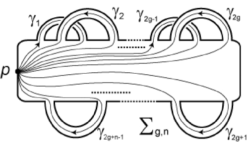
Figure 1. A spine $S$ of $\Sigma_{g,n}$

Next we recall the definition of sutured manifolds given by Gabai [8]. We use here a special class of sutured manifolds.

Definition 2.5.

A sutured manifold $(M,\gamma)$ is a compact oriented 3-manifold $M$ together with a subset $\gamma\subset\partial M$ which is a union of finitely many mutually disjoint annuli. For each component of $\gamma$, an oriented core circle called a suture is fixed, and we denote the set of sutures by $s(\gamma)$. Every component of $R(\gamma)=\partial M-{\rm Int\,}\gamma$ is oriented so that the orientations on $R(\gamma)$ are coherent with respect to $s(\gamma)$, i.e., the orientation of each component of $\partial R(\gamma)$, which is induced by that of $R(\gamma)$, is parallel to the orientation of the corresponding component of $s(\gamma)$. We denote by $R_{+}(\gamma)$ (resp. $R_{-}(\gamma)$) the union of those components of $R(\gamma)$ whose normal vectors point out of (resp. into) $M$. In this paper, we sometimes abbreviate $R_{+}(\gamma)$ (resp. $R_{-}(\gamma)$) to $R_{+}$ (resp. $R_{-}$). In the case that $(M,\gamma)$ is diffeomorphic to $(\Sigma\times[0,1],\partial\Sigma\times[0,1])$ where $\Sigma$ is a compact oriented surface, $(M,\gamma)$ is called a product sutured manifold.

Let $(M,i_{+},i_{-})\in\mathcal{C}_{g,n}$. If we consider a small regular neighborhood of $i_{+}(\partial\Sigma_{g,n})=i_{-}(\partial\Sigma_{g,n})$ in $\partial M$ to be $\gamma$, we can regard $(M,i_{+},i_{-})$ as a sutured manifold. However the converse is clearly not true in general. In the next section, we will determine which kinds of links give homology cylinders by considering their complementary sutured manifolds, which are defined as follows.

Definition 2.6.

Let $L$ be an oriented link in the 3-sphere $S^{3}$, and $\bar{R}$ a Seifert surface of $L$. Set $R:=\bar{R}\cap E(L)$, where $E(L)={\rm cl}(S^{3}-N(L))$ is the complement of a regular neighborhood of $L$, and $(P,\delta):=(N(R,E(L)),N(\partial R,\partial E(L)))$. We call $(P,\delta)$ the product sutured manifold for $R$. Let $(M,\gamma)=({\rm cl}(E(L)-P),{\rm cl}(\partial E(L)-\delta))$ with $R_{\pm}(\gamma)=R_{\mp}(\delta)$. We call $(M,\gamma)$ the complementary sutured manifold for $R$.

3. Homologically fibered links

Let $L$ be an oriented link in the 3-sphere $S^{3}$, and $\Delta_{L}(t)$ the normalized (one variable) Alexander polynomial of $L$, i.e., the lowest degree of $\Delta_{L}(t)$ is 0.

Definition 3.1.

An $n$-component oriented link $L$ in $S^{3}$ is said to be homologically fibered if $L$ satisfies the following two conditions:

1. The degree of $\Delta_{L}(t)$ is $2g+n-1$, where $g$ is the genus of a connected Seifert surface of $L$; and

2. $\Delta_{L}(0)=\pm 1$.

An $n$-component oriented link $L$ satisfying (i) is said to be rationally homologically fibered.

Hereafter links are always assumed to be oriented. We also assume $2g+n-1\geq 1$. Indeed the trivial knot is the only rationally homologically fibered link with $2g+n-1=0$.

A link $L$ is said to be fibered if $E(L)$ is the total space of a fiber bundle over $S^{1}$ whose fiber is given by a Seifert surface. It is well known that fibered links satisfy the conditions in Definition 3.1. Hence they are homologically fibered.

Let $L$ be an $n$-component link and $\Sigma_{g,n}$ the compact oriented surface that is diffeomorphic to a Seifert surface $R$ of $L$. We fix a diffeomorphism $\vartheta:\Sigma_{g,n}\stackrel{{\scriptstyle\cong}}{{\rightarrow}}R$ and denote by $(M,\gamma)$ the complementary sutured manifold for $R$. Then we may see that there are an orientation-preserving embedding $i_{+}:\Sigma_{g,n}\to\partial M$ and an orientation-reversing embedding $i_{-}:\Sigma_{g,n}\to\partial M$ with $i_{+}(\Sigma_{g,n})=R_{+}(\gamma)$ and $i_{-}(\Sigma_{g,n})=R_{-}(\gamma)$, where two embeddings $i_{\pm}$ are the composite maps of $\vartheta$ and the natural embeddings $\iota_{\pm}:R\hookrightarrow\partial M$:

If $i_{+},\,i_{-}:H_{1}(\Sigma_{g,n})\to H_{1}(M)$ are isomorphisms, we may regard $(M,\gamma)$ as a homology cylinder. The purpose of this section is to prove the next proposition.

Proposition 3.2.

Let $R$ be a Seifert surface of a link $L$ with a diffeomorphism $\vartheta:\Sigma_{g,n}\stackrel{{\scriptstyle\cong}}{{\rightarrow}}R$. If the complementary sutured manifold for $R$ is a $($rational$)$ homology cylinder, then $L$ is $($rationally$)$ homologically fibered. Conversely, if $L$ is $($rational$)$ homologically fibered, then the complementary sutured manifold for any minimal genus connected Seifert surface of $L$ gives a $($rational$)$ homology cylinder.

Remark 3.3.

• Aside from the name of homologically fibered links, the above fact was essentially mentioned in Crowell-Trotter [4].

• Suppose $L$ is a homologically fibered link and $M$ is the homology cylinder obtained from $L$ by the above procedure. If we change the diffeomorphism $\vartheta:\Sigma_{g,n}\xrightarrow{\cong}R$ into another one $\vartheta^{\prime}$, then the resulting homology cylinder is $(\vartheta^{-1}\circ\vartheta^{\prime})^{-1}\cdot M\cdot(\vartheta^{-1}\circ\vartheta^{\prime})\in\mathcal{C}_{g,n}$, where $\vartheta^{-1}\circ\vartheta^{\prime}\in\mathcal{M}_{g,n}$ is considered to be a homology cylinder as seen in Example 2.2.

For the proof of Proposition 3.2, we first set up our notation, following [1] and [29]. Consider the basis $\{\alpha_{i}:=[\gamma_{i}]\}$ $(1\leq i\leq 2g+n-1)$ of $H_{1}(\Sigma_{g,n};\mathbb{Z})\cong\mathbb{Z}^{2g+n-1}$ as shown in Figure 1. We may see that $R$ consists of a disk $D^{2}$ and bands $B_{i}$ $(1\leq i\leq 2g+n-1)$, where the cores of $B_{i}$ correspond to $\vartheta(\alpha_{i})$. For simplicity, we use $\alpha_{i}$ again instead of $\vartheta(\alpha_{i})$. See Figure 2 for the case of the trefoil.

Figure 2. Trefoil with the genus $1$ Seifert surface

Let $(P,\delta)$ be the product sutured manifold for $R$. The curves $\alpha_{1},\ldots,\alpha_{2g+n-1}$ of $R$ are projected onto curves $\alpha_{1}^{+},\ldots,\alpha_{2g+n-1}^{+}$ on $R_{+}(\delta)$ by $\iota_{+}$, and $\alpha_{1}^{-},\ldots,\alpha_{2g+n-1}^{-}$ on $R_{-}(\delta)$ by $\iota_{-}$. Choose a curve $\beta_{i}$ on the boundary of the regular neighborhood of the band $B_{i}$ so that each $\beta_{i}$ bounds a disk in $P$ that meets $\alpha_{i}$ at one point. The orientation of the disk and of $\beta_{i}$ are chosen such that the intersection number is +1. (See Figure 2, or [1, Figure 8.3].)

Lemma 3.4.

• The set $\{\alpha_{1}^{\varepsilon},\ldots,\alpha_{2g+n-1}^{\varepsilon},\beta_{1},\ldots,\beta_{2g+n-1}\}$ with $\varepsilon=+1\text{ or }-$ is a basis of $H_{1}(\partial M)=H_{1}(\partial P)\cong\mathbb{Z}^{4g+2n-2}$.

• $\{\alpha_{1}^{\varepsilon},\ldots,\alpha_{2g+n-1}^{\varepsilon}\}$ with $\varepsilon=+1\text{ or }-$ is a basis of $H_{1}(P)$ and $\{\beta_{1},\ldots,\beta_{2g+n-1}\}$ is a basis of $H_{1}(M)\cong\mathbb{Z}^{2g+n-1}$.

• $H_{\ast}(M)=0$ for $\ast\geq 2$.

Proof.

It is not difficult to show (1) and the first statement in (2). For the second one in (2), one may apply the Mayer-Vietoris sequence:

$$0=H_{2}(S^{3})\rightarrow H_{1}(\partial M)\xrightarrow{\phi}H_{1}(P)\oplus H_{1}(M)\rightarrow H_{1}(S^{3})=0.$$

Note that $\partial M=\partial P$ and $\phi(\beta_{i})=(0,\beta_{i})$. Then, the conclusion follows from (1).

In the exact sequence $H_{1}(\partial M)\to H_{1}(M)\to H_{1}(M,\partial M)\to 0$, the first map is surjective from (1) and (2). Thus $H_{1}(M,\partial M)=0$. By the Poincaré duality, we have $H_{2}(M)\cong H^{1}(M,\partial M)=0$. Clearly $H_{\ast}(M)=0$ for $\ast\geq 3$, and (3) holds. ∎

Let $\mathcal{S}$ be the Seifert matrix corresponding to the above basis of $H_{1}(R)$, namely $\mathcal{S}=(a_{jk})=(\text{lk}(\alpha^{-}_{j},\alpha_{k}))\,(1\leq j,\,k\leq 2g+n-1)$.

Lemma 3.5.

Let $\iota_{\pm}:R_{\pm}(\delta)\to M$ denote the inclusions. Then,

$$\iota_{+}(\alpha^{+}_{j})=\sum_{k=1}^{2g+n-1}a_{kj}\beta_{k}\hskip 14.22636pt\text{ and }\hskip 14.22636pt\iota_{-}(\alpha^{-}_{j})=\sum_{k=1}^{2g+n-1}a_{jk}\beta_{k}.$$

Proof.

See the proof of [1, Lemma 8.6] or [29, Page 53]. ∎

By Lemma 3.5, we have:

Lemma 3.6.

The maps $i_{\pm}:H_{1}(\Sigma_{g,n})\to H_{1}(M)$ $($resp. $i_{\pm}:H_{1}(\Sigma_{g,n};\mathbb{Q})\to H_{1}(M;\mathbb{Q}))$ are isomorphisms if and only if $\mathcal{S}$ is invertible over $\mathbb{Z}$ $($resp. over $\mathbb{Q})$.

Proof of Proposition 3.2.

Suppose that the complementary sutured manifold $M$ for $R$ is a rational homology cylinder. Then $\mathcal{S}$ is invertible over $\mathbb{Q}$ by Lemma 3.6 and $(\mathcal{S}^{T})^{-1}\mathcal{S}$ represents $\sigma(M)$, where $\mathcal{S}^{T}$ denotes the transpose of $\mathcal{S}$. By definition, we have $\Delta_{L}(t)=\det(t\mathcal{S}-\mathcal{S}^{T})$, and now

(3.1) $$\Delta_{L}(t)=\det(t\mathcal{S}-\mathcal{S}^{T})=\det(\mathcal{S}^{T})\det(t(\mathcal{S}^{T})^{-1}\mathcal{S}-I_{2g+n-1})$$

holds. Since $\det((\mathcal{S}^{T})^{-1}\mathcal{S})=1$, the polynomial $\det((t(\mathcal{S}^{T})^{-1}\mathcal{S}-I_{2g+n-1})$ is of degree $2g+n-1$ and so is $\Delta_{L}(t)$. Therefore $L$ is rationally homologically fibered. If moreover $M$ is a homology cylinder, then we have $\det(\mathcal{S})=\pm 1$ and $\Delta_{L}(0)=\det(-\mathcal{S}^{T})=\pm 1$. Hence $L$ is homologically fibered.

Conversely, let $L$ be a rationally homologically fibered link and $R$ be a minimal genus, say $g$, connected Seifert surface. Then, the degree of $\Delta_{L}(t)$ is $2g+n-1$. Since $\Delta_{L}(t)=\det(t\mathcal{S}-\mathcal{S}^{T})$ and $0\neq\Delta_{L}(0)=\det(-\mathcal{S}^{T})$, the complementary sutured manifold for $R$ is a rational homology cylinder by Lemma 3.6. Further, if $L$ is homologically fibered, we have $\pm 1=\Delta_{L}(0)=\det(-\mathcal{S}^{T})=\det(-\mathcal{S})$. This completes the proof. ∎

Example 3.7.

It is known ([3], [34]) that alternating links satisfy the condition (i) in Definition 3.1. Moreover it was shown by Murasugi [35] (see also 13.26 (c) in [1]) that an alternating link is fibered if and only if $\Delta_{L}(0)=\pm 1$. Therefore, if a homologically fibered link $L$ is not fibered, then it is non-alternating.

Example 3.8.

Let $p,\,q$ and $r$ be odd integers and let $P(p,q,r)$ be the pretzel knot of type $\{p,q,r\}$. See Figure 3. We assume that one of $p,\,q,\,r$, say $p$, is negative and the others are positive since our main objects are non-alternating knots (Example 3.7). It is well-known that the Alexander polynomial of $P(p,q,r)$ is given by

$$\frac{1}{4}\Big{(}(pq+qr+rp)(t^{2}-2t+1)+t^{2}+2t+1\Big{)}.$$

In the range of values: $-100<p\leq-3,\,3\leq q\leq r<100$, the pretzel knots of the following 22 types are homologically fibered knots.

$$\{-3,5,9\},\{-5,7,19\},\{-7,9,33\},\{-9,11,51\},\{-9,15,23\},\{-11,13,73\},$$

$$\{-13,15,99\},\{-15,21,53\},\{-19,33,45\},\{-21,27,95\},\{-23,37,61\},$$

$$\{-33,59,75\},\{-3,5,5\},\{-5,7,15\},\{-7,9,29\},\{-9,11,47\},\{-11,13,69\},$$

$$\{-13,15,95\},\{-15,25,37\},\{-25,35,87\},\{-29,51,67\},\{-37,59,99\}.$$

The minimal genus (genus 1) Seifert surface for the pretzel knot of this type is unique up to isotopy [16].

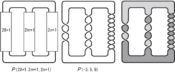
Figure 3. Standard diagram of Pretzel knots

Example 3.9.

Consider the pretzel knot of type $\{p,q,r,s,u\}$, where $p,\,q,\,r,\,s,\,u$ are odd integers. The leading coefficient of the Alexander polynomial is

$$\frac{1}{16}(pq+pr+ps+pu+qr+qs+qu+rs+ru+su+pqrs+pqru+pqsu+prsu+qrsu).$$

In the range of values: $-500<p\leq-3,\,3\leq q\leq r\leq s\leq u<500$, the following 8 types give the homologically fibered pretzel knots.

$$\{-3,9,9,9,85\},\{-5,15,15,15,411\},\{-7,17,17,45,261\},$$

$$\{-9,15,35,71,467\},\{-33,75,127,151,403\},\{-39,113,161,165,221\},$$

$$\{-9,23,27,35,411\},\{-37,107,107,179,363\}.$$

In the range of values: $$-300<p\leq q\leq-3,\,3\leq r\leq s\leq u<300$$, the following 15 types give the homologically fibered pretzel knots.

$$\{-15,-3,5,5,125\},\{-5,-5,3,19,159\},\{-69,-5,7,15,151\},$$

$$\{-31,-7,9,17,177\},\{-27,-11,9,85,205\},\{-15,-3,5,5,129\},$$

$$\{-5,-5,3,19,163\},\{-53,-5,7,15,91\},\{-177,-5,7,31,31\},$$

$$\{-257,-5,7,19,99\},\{-235,-7,17,17,33\},\{-15,-11,13,13,265\},$$

$$\{-275,-11,13,109,117\},\{-37,-33,23,111,207\},\{-121,-33,39,107,279\}.$$

Example 3.10.

Let $K$ be the trefoil knot, which is fibered. We take the basis $\{\alpha_{1},\alpha_{2}\}$ of $H_{1}(R)$ for the minimal genus Seifert surface $R$ as in Figure 4. We cut the band corresponding to $\alpha_{2}$, make it knotted, and paste to the original part again, then we have a new knot with a Seifert surface of the same genus. Just before pasting, we twist the band so that the Seifert matrix (linking number) does not change, then we can obtain a knot whose Alexander polynomial is the same as $K$. By this method, we can obtain many homologically fibered knots.

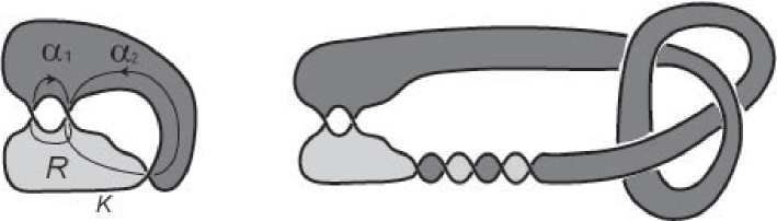
Figure 4. Making a new homologically fibered knot

Example 3.11.

It is known that a knot $K$ with 11 or fewer crossings is fibered if and only if $K$ is homologically fibered. Among 12 crossing knots there are thirteen knots which are not fibered but homologically fibered. See Friedl-Kim[7] for the detail.

4. Invariants of homology cylinders and fibering obstructions of links

In this section, we review some invariants of homology cylinders from [37]. We begin by summarizing our notation. For a matrix $A$ with entries in a ring $\mathcal{R}$, and a ring homomorphism $\rho:\mathcal{R}\to\mathcal{R}^{\prime}$, we denote by ${}^{\rho}A$ the matrix obtained from $A$ by applying $\rho$ to each entry. When $\mathcal{R}=\mathbb{Z}G$ (or its fractional field if it exists) for a group $G$, we denote by $\overline{A}$ the matrix obtained from $A$ by applying the involution induced from $(x\mapsto x^{-1},\ x\in G)$ to each entry. For a module $\mathcal{M}$, we write $\mathcal{M}^{n}$ for the module of column vectors with $n$ entries. For a finite cell complex $X$, we denote by $\widetilde{X}$ its universal covering. We take a base point $p$ of $X$. The group $\pi:=\pi_{1}(X,p)$ acts on $\widetilde{X}$ from the right as its deck transformations. Then the cellular chain complex $C_{\ast}(\widetilde{X})$ of $\widetilde{X}$ becomes a right $\mathbb{Z}\pi$-module. For each left $\mathbb{Z}\pi$-algebra $\mathcal{R}$, the twisted chain complex $C_{\ast}(X;\mathcal{R})$ is given by the tensor product of the right $\mathbb{Z}\pi$-module $C_{\ast}(\widetilde{X})$ and the left $\mathbb{Z}\pi$-module $\mathcal{R}$, so that $C_{\ast}(X;\mathcal{R})$ and $H_{\ast}(X;\mathcal{R})$ are right $\mathcal{R}$-modules.

Let $M=(M,i_{+},i_{-})\in\mathcal{C}_{g,n}^{\mathbb{Q}}$ and let $\rho_{\Gamma}:\pi_{1}(M)\to\Gamma$ be a homomorphism whose target $\Gamma$ is a poly-torsion-free abelian $($PTFA$)$ group, where a group $\Gamma$ is said to be PTFA if it has a sequence

$$\Gamma=\Gamma_{0}\triangleright\Gamma_{1}\triangleright\cdots\triangleright\Gamma_{n}=\{1\}$$

whose successive quotients $\Gamma_{i}/\Gamma_{i+1}$ $(i\geq 0)$ are all torsion-free abelian. Using a PTFA group $\Gamma$ has an advantage that its group ring $\mathbb{Z}\Gamma$ (or $\mathbb{Q}\Gamma$) is an Ore domain so that it is embedded into the right field

$$\mathcal{K}_{\Gamma}:=\mathbb{Z}\Gamma(\mathbb{Z}\Gamma-\{0\})^{-1}=\mathbb{Q}\Gamma(\mathbb{Q}\Gamma-\{0\})^{-1}$$

of fractions. We refer to Cochran-Orr-Teichner [2, Section 2] and Passman [36] for generalities of PTFA groups and localizations of their group rings. A typical example of PTFA groups associated with $M$ is the free part $\Gamma=H_{1}(M)/\mbox{(torsion)}\cong\mathbb{Z}^{2g+n-1}$ of $H_{1}(M)$, where $\mathcal{K}_{\Gamma}$ is isomorphic to the field of rational functions with $2g+n-1$ variables. The following lemma can be verified by applying Cochran-Orr-Teichner [2, Proposition 2.10]. However we here give a proof for later use.

Lemma 4.1.

The maps $i_{\pm}:H_{\ast}(\Sigma_{g,n},p;i_{\pm}^{\ast}\mathcal{K}_{\Gamma})\to H_{\ast}(M,p;\mathcal{K}_{\Gamma})$ are isomorphisms as right $\mathcal{K}_{\Gamma}$-vector spaces.

Proof.

For the proof, it suffices to show that $H_{\ast}(M,i_{+}(\Sigma_{g,n});\mathcal{K}_{\Gamma})=0$. Since the spine $S$ fixed in Section 2 is a deformation retract of $\Sigma_{g,n}$ relative to $p$, we have $H_{\ast}(M,i_{+}(\Sigma_{g,n});\mathcal{K}_{\Gamma})=H_{\ast}(M,i_{+}(S);\mathcal{K}_{\Gamma})$. Now we compute the latter.

Triangulate $\Sigma_{g,n}$ smoothly, so that the spine $S$ is the union of its edges. By gluing two copies of this triangulated surface, we obtain a triangulation $\mathfrak{t}$ of $\partial M$. A theorem of Cairns and Whitehead shows that there exists a triangulation $\widehat{\mathfrak{t}}$ of the entire $M$ which extends $\mathfrak{t}$. Starting from a 2-simplex in $\partial M$, we can deform $M$ onto a subcomplex $\widehat{\mathfrak{t}}$ of its 2-skeleton. In this deformation, the 1-skeleton is fixed pointwise. Take a maximal tree $T$ of $\mathfrak{t}$ such that $T$ includes all but one sub-edges of each loop of $S$. We extend $T$ to a maximal tree $\widetilde{T}$ of $\widetilde{\mathfrak{t}}$ and collapse $\widetilde{T}$ to a point. Then we obtain a 2-dimensional CW-complex $M^{\prime}$ having only one vertex. By construction, the bouquet $i_{+}(S)$ is mapped onto a bouquet $S^{\prime}$ in $M^{\prime}$ with a natural one-to-one correspondence between their loops, and $(M^{\prime},S^{\prime})$ is simple homotopy equivalent to $(M,i_{+}(S))$. ¿From this cell structure, we can read a presentation of $\pi_{1}(M)=\pi_{1}(M^{\prime})$ as

(4.1) $$\langle y_{1},\ldots,y_{k},i_{+}(\gamma_{1}),\ldots,i_{+}(\gamma_{2g+n-1})\mid s_{1},\ldots,s_{k}\rangle$$

for some $k$, where we identify $i_{+}(\gamma_{j})$ $(1\leq j\leq 2g+n-1)$ with its image in $M^{\prime}$.

We have $H_{\ast}(M,i_{+}(S);\mathcal{K}_{\Gamma})=H_{\ast}(M^{\prime},S^{\prime};\mathcal{K}_{\Gamma})$. The relative complex $(M^{\prime},S^{\prime})$ consists of only the same number of 1-cells and 2-cells, so that the relative chain complex $C_{\ast}(M^{\prime},S^{\prime};\mathcal{K}_{\Gamma})$ is of the form

$$0\longrightarrow(\mathcal{K}_{\Gamma})^{k}\stackrel{{\scriptstyle{}^{\rho_{\Gamma}}J\cdot}}{{\longrightarrow}}(\mathcal{K}_{\Gamma})^{k}\longrightarrow 0$$

with $J:=\overline{\left({\displaystyle\frac{\partial s_{j}}{\partial y_{i}}}\right)}_{1\leq i,j\leq k}$. The matrix ${}^{\rho_{\Gamma}}J$ has its entries in $\mathbb{Z}\Gamma$. To check the invertibility over $\mathcal{K}_{\Gamma}$ of this matrix, we apply the augmentation map $\mathfrak{a}:\mathbb{Z}\Gamma\to\mathbb{Z}$ to each entry. Then we obtain a presentation matrix of $H_{1}(M,i_{+}(\Sigma_{g,n}))$. Since $H_{1}(M,i_{+}(\Sigma_{g,n});\mathbb{Q})=0$, the matrix ${}^{\mathfrak{a}\circ\rho_{\Gamma}}J$ is invertible over $\mathbb{Q}$. Then it follows from Strebel [38, Section 1] that ${}^{\rho_{\Gamma}}J$ is invertible over $\mathcal{K}_{\Gamma}$. ($\Gamma$ belongs to the class $D(\mathbb{Z})$ in the notation of [38].) This completes the proof ∎

We use Lemma 4.1 to construct the following two invariants of rational homology cylinders. The first one is the Magnus matrix, which was defined in [37]. We have

$$H_{1}(\Sigma_{g,n},p;i_{\pm}^{\ast}\mathcal{K}_{\Gamma})\cong H_{1}(S,p;i_{\pm}^{\ast}\mathcal{K}_{\Gamma})=C_{1}(\widetilde{S})\otimes_{\pi_{1}(\Sigma_{g,n})}i_{\pm}^{\ast}\mathcal{K}_{\Gamma}\cong\mathcal{K}_{\Gamma}^{2g+n-1}$$

with a basis

$$\{\widetilde{\gamma}_{1}\otimes 1,\ldots,\widetilde{\gamma}_{2g+n-1}\otimes 1\}\subset C_{1}(\widetilde{S})\otimes_{\pi_{1}(\Sigma_{g,n})}i_{\pm}^{\ast}\mathcal{K}_{\Gamma}$$

as a right $\mathcal{K}_{\Gamma}$-module. Here we fix a lift $\widetilde{p}$ of $p$ as a base point of $\widetilde{S}$, and denote by $\widetilde{\gamma}_{i}$ the lift of the oriented loop $\gamma_{i}$.

Definition 4.2.

For $M=(M,i_{+},i_{-})\in\mathcal{C}_{g,n}^{\mathbb{Q}}$, the Magnus matrix

$$r_{\Gamma}(M)\in GL(2g+n-1,\mathcal{K}_{\Gamma})$$

of $M$ is defined as the representation matrix of the right $\mathcal{K}_{\Gamma}$-isomorphism

$$\mathcal{K}_{\Gamma}^{2g+n-1}\cong H_{1}(\Sigma_{g,n},p;i_{-}^{\ast}\mathcal{K}_{\Gamma})\xrightarrow[i_{-}]{\cong}H_{1}(M,p;\mathcal{K}_{\Gamma})\xrightarrow[i_{+}^{-1}]{\cong}H_{1}(\Sigma_{g,n},p;i_{+}^{\ast}\mathcal{K}_{\Gamma})\cong\mathcal{K}_{\Gamma}^{2g+n-1},$$

where the first and the last isomorphisms use the bases mentioned above.

Example 4.3.

For $(\Sigma_{g,n}\times[0,1],\mathrm{id}\times 1,\varphi\times 0)\in\mathcal{M}_{g,n}\subset\mathcal{C}_{g,n}$, we can check that

$$r_{\Gamma}((\Sigma_{g,n}\times[0,1],\mathrm{id}\times 1,\varphi\times 0))=\overline{\sideset{{}^{\rho_{\Gamma}}\!}{}{\mathop{\left({\displaystyle\frac{\partial\varphi(\gamma_{j})}{\partial\gamma_{i}}}\right)}\nolimits}}_{1\leq i,j\leq 2g+n-1}$$

from the definition or by using Proposition 4.5 below. ¿From this, we see that $r_{\Gamma}$ extends the Magnus representation of $\mathcal{M}_{g,1}$ in Morita [33].

Next we introduce a torsion invariant. Since the relative complex $C_{\ast}(M,i_{+}(\Sigma_{g,n});\mathcal{K}_{\Gamma})$ obtained from any cell decomposition of $(M,i_{+}(\Sigma_{g,n}))$ is acyclic by Lemma 4.1, we can consider its torsion $\tau(C_{\ast}(M,i_{+}(\Sigma_{g,n});$ $\mathcal{K}_{\Gamma}))$. We refer to Milnor [32] and Turaev [39] for generalities of torsions and related groups from algebraic K-theory. Recall that torsions are invariant under simple homotopy equivalences. In particular, they are topological invariants.

Definition 4.4.

The $\Gamma$-torsion of $M=(M,i_{+},i_{-})\in\mathcal{C}_{g,n}^{\mathbb{Q}}$ is given by

$$\tau_{\Gamma}^{+}(M):=\tau(C_{\ast}(M,i_{+}(\Sigma_{g,n});\mathcal{K}_{\Gamma}))\in K_{1}(\mathcal{K}_{\Gamma})/\pm\rho_{\Gamma}(\pi_{1}(M)).$$

Now we recall a method for computing $r_{\Gamma}(M)$ and $\tau_{\Gamma}^{+}(M)$ by following [37, Section 3.2], which is based on the one for the Gassner matrix (using commutative rings) of a string link by Kirk-Livingston-Wang [26] and Le Dimet [27, Section 1.1].

Let $(M,i_{+},i_{-})\in\mathcal{C}_{g,n}^{\mathbb{Q}}$. An admissible presentation of $\pi_{1}(M)$ is defined to be the one of the form

(4.2) $$\langle i_{-}(\gamma_{1}),\ldots,i_{-}(\gamma_{2g+n-1}),z_{1},\ldots,z_{l},i_{+}(\gamma_{1}),\ldots,i_{+}(\gamma_{2g+n-1})\mid r_{1},\ldots,r_{2g+n-1+l}\rangle$$

for some integer $l$. That is, it is a finite presentation with deficiency $2g+n-1$ whose generating set contains $i_{-}(\gamma_{1}),\ldots,i_{-}(\gamma_{2g+n-1}),i_{+}(\gamma_{1}),\ldots,i_{+}(\gamma_{2g+n-1})$ and is ordered as above. One of the possible constructions of admissible presentations is obtained from the presentation (4.1) by adding generators $i_{-}(\gamma_{1}),\ldots,i_{-}(\gamma_{2g+n-1})$ together with relations. (There also exists a construction using Morse theory.)

Given an admissible presentation of $\pi_{1}(M)$ as in (4.2), we define $(2g+n-1)\times(2g+n-1+l)$, $l\times(2g+n-1+l)$ and $(2g+n-1)\times(2g+n-1+l)$ matrices $A,B,C$ over $\mathbb{Z}\pi_{1}(M)$ by

$$A=\overline{\left(\frac{\partial r_{j}}{\partial i_{-}(\gamma_{i})}\right)}_{\begin{subarray}{c}{}1\leq i\leq 2g+n-1\\ 1\leq j\leq 2g+n-1+l\end{subarray}},\ B=\overline{\left(\frac{\partial r_{j}}{\partial z_{i}}\right)}_{\begin{subarray}{c}{}1\leq i\leq l\\ 1\leq j\leq 2g+n-1+l\end{subarray}},\ C=\overline{\left(\frac{\partial r_{j}}{\partial i_{+}(\gamma_{i})}\right)}_{\begin{subarray}{c}{}1\leq i\leq 2g+n-1\\ 1\leq j\leq 2g+n-1+l\end{subarray}}.$$

Proposition 4.5.

As matrices with entries in $\mathcal{K}_{\Gamma}$, we have the following.

• The square matrix $\sideset{{}^{\rho_{\Gamma}}\!\!}{}{\mathop{\begin{pmatrix}A\\ B\end{pmatrix}}\nolimits}$ is invertible and $\tau_{\Gamma}^{+}(M)=\sideset{{}^{\rho_{\Gamma}}\!\!}{}{\mathop{\begin{pmatrix}A\\ B\end{pmatrix}}\nolimits}$.

• $r_{\Gamma}(M)=-{}^{\rho_{\Gamma}}C\sideset{{}^{\rho_{\Gamma}}\!\!}{{}^{-1}}{\mathop{\begin{pmatrix}A\\ B\end{pmatrix}}\nolimits}\begin{pmatrix}I_{2g+n-1}\\ 0_{(l,2g+n-1)}\end{pmatrix}$.

In particular, the invariants $\tau_{\Gamma}^{+}(M)$ and $r_{\Gamma}(M)$ are computable from any admissible presentation of $\pi_{1}(M)$.

Proof.

(1) For an admissible presentation of $\pi_{1}(M)=\pi_{1}(M^{\prime})$ obtained from (4.1), the torsion $\tau_{\Gamma}^{+}(M)$ is given by the matrix ${}^{\rho_{\Gamma}}J$. Hence our claim holds in this case.

Given any admissible presentation $P$ of $\pi_{1}(M)$ as in (4.2), we construct a 2-complex $X(P)$ having one 0-cell as a basepoint, $(4g+2n-2+l)$ 1-cells indexed by the generators and $(2g+n-1+l)$ 2-cells indexed by the relations and attached according to the words. Then we can use a theorem of Harlander-Jensen [22, Theorem 3] with the fact that the deficiency of $\pi_{1}(M)$ is $2g+n-1$ (see Epstein [5, Lemmas 1.2, 2,2]) to show that $X(P)$ and $M^{\prime}$ are homotopy equivalent. In fact, there exists a basepoint preserving cellular map $f:X(P)\to M^{\prime}$ which is a homotopy equivalence and maps the union $S_{0}$ of the 1-cells of $P_{0}$ corresponding to $i_{+}(\gamma_{1}),\ldots,i_{+}(\gamma_{2g+n-1})$ homeomorphically onto $S^{\prime}$. Let $M_{f}$ be the mapping cylinder of $f$. We have

$$\tau_{\Gamma}^{+}(M) =\tau(C_{\ast}(M,i_{+}(\Sigma_{g,n});\mathcal{K}_{\Gamma}))=\tau(C_{\ast}(M,i_{+}(S);\mathcal{K}_{\Gamma}))$$

$$=\tau(C_{\ast}(M^{\prime},S^{\prime};\mathcal{K}_{\Gamma}))=\tau(C_{\ast}(M_{f},S^{\prime};\mathcal{K}_{\Gamma}))=\tau(C_{\ast}(M_{f},S_{0}\times[0,1];\mathcal{K}_{\Gamma}))$$

$$=\tau(C_{\ast}(M_{f},S_{0};\mathcal{K}_{\Gamma}))=\tau(C_{\ast}(M_{f},X(P);\mathcal{K}_{\Gamma}))\tau(C_{\ast}(X(P),S_{0};\mathcal{K}_{\Gamma}))$$

where we repeatedly used the multiplicativity of torsions. (For example, we have

$$\tau(C_{\ast}(M,i_{+}(S);\mathcal{K}_{\Gamma}))=\tau(C_{\ast}(M,i_{+}(\Sigma_{g,n});\mathcal{K}_{\Gamma}))\tau(C_{\ast}(i_{+}(\Sigma_{g,n}),i_{+}(S);\mathcal{K}_{\Gamma}))$$

with $\tau(C_{\ast}(i_{+}(\Sigma_{g,n}),i_{+}(S);\mathcal{K}_{\Gamma}))=1$ since $i_{+}(\Sigma_{g,n})$ is simple homotopy equivalent to $i_{+}(S)$.)

We now compute $\tau(C_{\ast}(X(P),S_{0};\mathcal{K}_{\Gamma}))$. As in the case of the complex $(M^{\prime},S^{\prime})$, the relative complex $(X(P),S_{0})$ consists of only the same number of 1-cells and 2-cells. Thus $\tau(C_{\ast}(X(P),S_{0};\mathcal{K}_{\Gamma}))$ is given by $\sideset{{}^{\rho_{\Gamma}}\!\!}{}{\mathop{\begin{pmatrix}A\\ B\end{pmatrix}}\nolimits}$, which is a square matrix over $\mathbb{Z}\Gamma$. By an argument similar to the matrix $J$ in the proof of Lemma 4.1, we can check that this matrix is invertible over $\mathcal{K}_{\Gamma}$.

If $M$ is an irreducible 3-manifold, it is a Haken manifold since $|H_{1}(M)|=\infty$. Waldhausen’s theorem [41, Theorems 19.4, 19.5] shows that the Whitehead group $Wh(\pi)=K_{1}(\mathbb{Z}\pi_{1}(M))/\pm\pi_{1}(M)$ of $\pi_{1}(M)$ vanishes. Hence $X(P)$, $M^{\prime}$ and $M_{f}$ are simple homotopy equivalent and we have $\tau(C_{\ast}(M_{f},X(P);\mathcal{K}_{\Gamma}))=1$. The second claim of (1) follows in this case.

If $M$ is not irreducible, we can check that $M$ is a connected sum of a Haken manifold $M_{0}$ containing $\partial M$ and a (possibly reducible) rational homology 3-sphere $M_{2}$. Since any homomorphism from $\pi_{1}(M_{2})$ to a PTFA group $\Gamma$ is trivial, the homomorphism $\rho_{\Gamma}$ factors through $\pi_{1}(M_{1})$, whose Whitehead group vanishes as mentioned above. Now $\tau(C_{\ast}(M_{f},X(P);\mathcal{K}_{\Gamma}))$ is the image of the Whitehead torsion $\tau(C_{\ast}(M_{f},X(P);\mathbb{Z}\pi_{1}(M)))\in Wh(\pi_{1}(M))$ by $\rho_{\Gamma}$. It must be trivial since it passes through $Wh(\pi_{1}(M_{1}))=0$. This completes the proof.

(2) The proof is almost identical to that in [37, Proposition 3.9], and here we omit it. ∎

The $\Gamma$-torsion and the Magnus matrix can be used as fibering obstructions of a homologically fibered link as follows. If a link is fibered, the complementary sutured manifold for each minimal genus Seifert surface is a product sutured manifold, whose $\Gamma$-torsion is trivial for any $\mathcal{K}_{\Gamma}$. Together with Example 4.3, we have:

Theorem 4.6.

• Suppose a homologically fibered link has a minimal genus Seifert surface which gives a homology cylinder having non-trivial $\Gamma$-torsion for some PTFA group $\Gamma$, then it is not fibered.

• Let $M$ be a homology cylinder obtained from a minimal genus Seifert surface of a fibered link. Then all the entries of the Magnus matrix $r_{\Gamma}(M)$ are in $\mathbb{Z}\Gamma$.

Example 4.7.

Let $K=P(-3,5,9)$, which is a homologically fibered knot as seen in Example 3.8. We take a Seifert surface of $K$ and its spine as in Figure 6, where the darker color means the $+$-side.

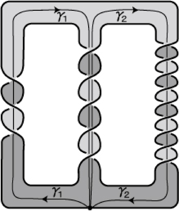
Figure 5. A Seifert surface of $P(-3,5,9)$ and its spine

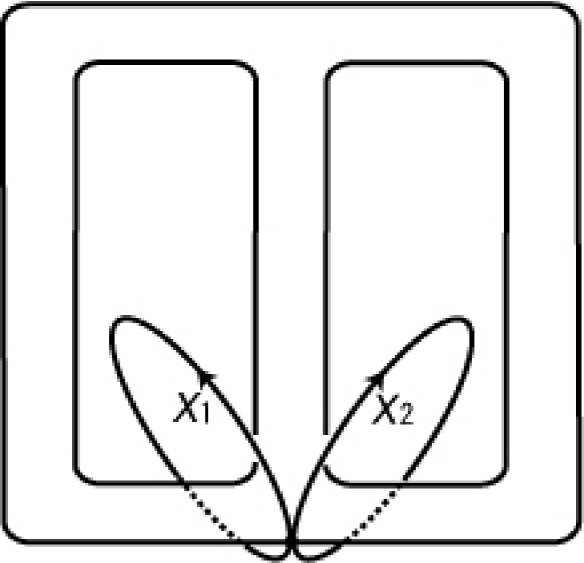
Figure 6. A basis of $\pi_{1}(M)$

The loops $x_{1},x_{2}$ in Figure 6 form a basis of $\pi_{1}(M)$ of the complementary sutured manifold $M$. They are oriented according to Figure 2. A direct computation shows that

$$i_{-}(\gamma_{1})=x_{1}^{-1}(x_{2}x_{1})^{2},\ \ i_{-}(\gamma_{2})=x_{2}^{4}(x_{2}x_{1})^{3},\ \ i_{+}(\gamma_{1})=x_{1}^{-2}(x_{1}x_{2})^{3},\ \ i_{+}(\gamma_{2})=x_{2}^{5}(x_{1}x_{2})^{2}$$

and we obtain an admissible presentation

$${\small\left\langle\begin{array}[]{c|l}i_{-}(\gamma_{1}),i_{-}(\gamma_{2}),x_{1},x_{2},i_{+}(\gamma_{1}),i_{+}(\gamma_{2})&\begin{array}[]{l}i_{-}(\gamma_{1})(x_{1}^{-1}x_{2}^{-1})^{2}x_{1},\ i_{-}(\gamma_{2})(x_{1}^{-1}x_{2}^{-1})^{3}x_{2}^{-4},\\ i_{+}(\gamma_{1})(x_{2}^{-1}x_{1}^{-1})^{3}x_{1}^{2},\ i_{+}(\gamma_{2})(x_{2}^{-1}x_{1}^{-1})^{2}x_{2}^{-5}\end{array}\end{array}\right\rangle}$$

of $\pi_{1}(M)$. $H_{1}(M)$ is the free abelian group generated by $t_{1}:=[x_{1}]$ and $t_{2}:=[x_{2}]$ and the natural homomorphism $\rho_{\Gamma}:\pi_{1}(M)\to H_{1}(M)=:\Gamma$ maps

$$i_{-}(\gamma_{1})\mapsto t_{1}t_{2}^{2},\quad i_{-}(\gamma_{2})\mapsto t_{1}^{3}t_{2}^{7},\quad i_{+}(\gamma_{1})\mapsto t_{1}t_{2}^{3},\quad i_{+}(\gamma_{2})\mapsto t_{1}^{2}t_{2}^{7}.$$

Now $\mathcal{K}_{\Gamma}$ is isomorphic to the field of rational functions with variables $t_{1}$ and $t_{2}$. We have

$${}^{\rho_{\Gamma}}A=\begin{pmatrix}I_{2}&0_{(2,2)}\end{pmatrix},\qquad{}^{\rho_{\Gamma}}B=\begin{pmatrix}G_{1}&G_{2}\end{pmatrix},\qquad{}^{\rho_{\Gamma}}C=\begin{pmatrix}0_{(2,2)}&I_{2}\end{pmatrix},$$

where

$$G_{1} =\begin{pmatrix}t_{1}-t_{1}t_{2}^{-1}-t_{2}^{-2}&-t_{1}^{-2}t_{2}^{-7}-t_{1}^{-1}t_{2}^{-6}-t_{2}^{-5}\\ -t_{1}-t_{2}^{-1}&-t_{1}^{-2}t_{2}^{-6}-t_{1}^{-1}t_{2}^{-5}-t_{2}^{-4}-t_{2}^{-3}-t_{2}^{-2}-t_{2}^{-1}-1\end{pmatrix},$$

$$G_{2} =\begin{pmatrix}t_{1}-t_{1}t_{2}^{-1}-t_{2}^{-2}&-t_{1}^{-1}t_{2}^{-6}-t_{2}^{-5}\\ -t_{1}^{-1}t_{2}^{-2}-t_{1}-t_{2}^{-1}&-t_{1}^{-2}t_{2}^{-6}-t_{1}^{-1}t_{2}^{-5}-t_{2}^{-4}-t_{2}^{-3}-t_{2}^{-2}-t_{2}^{-1}-1\end{pmatrix}.$$

Thus $\tau_{\Gamma}^{+}(M)=\sideset{{}^{\rho_{\Gamma}}\!\!}{}{\mathop{\begin{pmatrix}A\\ B\end{pmatrix}}\nolimits}=\begin{pmatrix}I_{2}&0_{(2,2)}\\ G_{1}&G_{2}\end{pmatrix}=G_{2}\in K_{1}(\mathcal{K}_{\Gamma})/\pm\rho_{\Gamma}(\pi_{1}(M))$, which is non-trivial because

$$\det(\tau_{\Gamma}^{+}(M))=\det(G_{2})=-t_{1}^{-1}t_{2}^{-6}-t_{1}+t_{2}^{-4}+t_{2}^{-3}+t_{2}^{-2}$$

is not a monomial. This shows that $P(-3,5,9)$ is not fibered by Theorem 4.6 (1). The Magnus matrix $r_{\Gamma}(M)$ is given by

$${\Large\left(\begin{array}[]{cc}\frac{-1-t_{1}t_{2}+t_{1}t_{2}^{2}-t_{1}^{2}t_{2}^{4}-t_{1}^{2}t_{2}^{5}-t_{1}^{2}t_{2}^{6}+t_{1}^{3}t_{2}^{8}}{t_{1}t_{2}^{2}(1-t_{1}t_{2}^{2}-t_{1}t_{2}^{3}-t_{1}t_{2}^{4}+t_{1}^{2}t_{2}^{6})}&\frac{-1-t_{1}t_{2}-t_{1}^{2}t_{2}^{2}-t_{1}^{2}t_{2}^{3}-t_{1}^{2}t_{2}^{4}-t_{1}^{2}t_{2}^{5}-t_{1}^{2}t_{2}^{6}}{t_{1}^{3}t_{2}^{7}(1-t_{1}t_{2}^{2}-t_{1}t_{2}^{3}-t_{1}t_{2}^{4}+t_{1}^{2}t_{2}^{6})}\\ &\\ \frac{t_{2}^{2}(1+t_{1}t_{2}-t_{1}t_{2}^{2})}{1-t_{1}t_{2}^{2}-t_{1}t_{2}^{3}-t_{1}t_{2}^{4}+t_{1}^{2}t_{2}^{6}}&\frac{1+t_{1}t_{2}+t_{1}^{2}t_{2}^{2}+t_{1}^{2}t_{2}^{3}-t_{1}^{3}t_{2}^{5}-t_{1}^{3}t_{2}^{6}-t_{1}^{3}t_{2}^{7}+t_{1}^{4}t_{2}^{9}}{t_{1}^{2}t_{2}^{3}(1-t_{1}t_{2}^{2}-t_{1}t_{2}^{3}-t_{1}t_{2}^{4}+t_{1}^{2}t_{2}^{6})}\end{array}\right),}$$

which also indicates the non-fiberedness of $P(-3,5,9)$ since all the entries of $r_{\Gamma}(M)$ should be Laurent polynomials by Theorem 4.6(2) if it were fibered .

5. Twisted homology and torsions of rationally homologically fibered link exteriors

In this section, we see that the invariants defined in Section 4 make up torsions of exteriors of rationally homologically fibered links under special choices of PTFA groups $\Gamma$. Before that, we observe generalities of torsions of link exteriors.

Let $L$ be an $n$-component link. Assume that the $($one variable$)$ Alexander polynomial $\Delta_{L}(t)$ of $L$ is not equal to zero. Then the Wirtinger presentation gives a presentation of $\pi_{1}(E(L))$ with deficiency $0$. It is known that we can drop any one of the relations. Let $Q_{0}$ be such a presentation of the form

$$\langle y_{1},\ldots,y_{m+1}\mid s_{1},\ldots,s_{m}\rangle.$$

It is also known that the CW-complex $X(Q_{0})$ constructed as in the proof of Proposition 4.5 has the same simple homotopy type as the link exterior $E(L)$.

Let $\rho_{\Gamma}:\pi_{1}(E(L))\to\Gamma$ be an epimorphism whose target $\Gamma\neq\{1\}$ is PTFA and let $\rho:\pi_{1}(E(L))\to\langle t\rangle\cong\mathbb{Z}$ be the homomorphism sending each oriented meridian to $t$. The following proposition gives a sufficient condition for the torsion $\tau_{\Gamma}(E(L))=\tau(C_{\ast}(E(L);\mathcal{K}_{\Gamma}))$ of $E(L)$ to be defined.

Proposition 5.1.

If the $($one variable$)$ Alexander polynomial $\Delta_{L}(t)$ of $L$ is not equal to zero and $\rho$ factors through $\rho_{\Gamma}$, then $H_{\ast}(E(L);\mathcal{K}_{\Gamma})=0$.

Proof.

The chain complex $C_{\ast}(X(Q_{0});\mathbb{Z}\Gamma)$ is of the form

(5.1) $$0\longrightarrow(\mathbb{Z}\Gamma)^{m}\xrightarrow{{}^{\rho_{\Gamma}}J\cdot}(\mathbb{Z}\Gamma)^{m+1}\xrightarrow{{}^{\rho_{\Gamma}}\begin{pmatrix}1-y_{1}^{-1},\ldots,1-y_{m+1}^{-1}\end{pmatrix}\cdot}\mathbb{Z}\Gamma\longrightarrow 0,$$

where $J=\overline{\left(\displaystyle\frac{\partial s_{j}}{\partial y_{i}}\right)}_{\begin{subarray}{c}{}1\leq i\leq m+1\\ 1\leq j\leq m\end{subarray}}$. Now the assumption $\Delta_{L}(t)\neq 0$ implies that $H_{\ast}(E(L);\mathcal{K}_{\langle t\rangle})=0$. In particular, ${}^{\rho}J\cdot:(\mathbb{Z}\langle t\rangle)^{m}\to(\mathbb{Z}\langle t\rangle)^{m+1}$ is injective. Since PTFA groups are locally indicable, it follows from Friedl [6, Proposition 6.4] that the second map of (5.1) is injective. It is still injective when we apply $\otimes_{\Gamma}\mathcal{K}_{\Gamma}$. The third map of (5.1) is clearly surjective after applying $\otimes_{\Gamma}\mathcal{K}_{\Gamma}$. Hence $H_{\ast}(E(L);\mathcal{K}_{\Gamma})=H_{\ast}(X(Q_{0});\mathcal{K}_{\Gamma})=0$ holds. ∎

Remark 5.2.

In the above argument, we can replace $\rho$ by any other homomorphism $\rho^{\prime}:\pi_{1}(E(L))\to\mathbb{Z}$ satisfying $H_{\ast}(E(L);\mathcal{K}_{\mathbb{Z}})=0$, where $\mathcal{K}_{\mathbb{Z}}$ is twisted by $\rho^{\prime}$. In fact, since the multivariable Alexander polynomial of $L$ is non-trivial (see [25, Proposition 7.3.10], for example), we can use McMullen’s argument [30, Theorem 4.1] to show that $H_{\ast}(E(L);\mathcal{K}_{\mathbb{Z}})=0$ for generic $\rho^{\prime}\neq 0$. We also remark that by the definition of PTFA groups, there exists at least one homomorphism $\Gamma\to\mathbb{Z}$, whose composition with $\rho_{\Gamma}$ is non-trivial.

Hereafter we assume that $H_{\ast}(E(L);\mathcal{K}_{\Gamma})=0$. By using the cell structure of $X(Q_{0})$, the torsion $\tau_{\Gamma}(E(L))$ is given by

$$\tau_{\Gamma}(E(L)) =\tau_{\Gamma}(X(Q_{0}))=({}^{\rho_{\Gamma}}J)_{i}\cdot(1-\rho_{\Gamma}(y_{i}^{-1}))^{-1}$$

$$\in K_{1}(\mathcal{K}_{\Gamma})/\pm\rho_{\Gamma}(\pi_{1}(E(L)))=K_{1}(\mathcal{K}_{\Gamma})/\pm\Gamma,$$

where $1\leq i\leq m+1$ is chosen so that $\rho_{\Gamma}(y_{i})\neq 1$ and $({}^{\rho_{\Gamma}}J)_{i}$ is obtained from ${}^{\rho_{\Gamma}}J$ by deleting its $i$-th row (see Friedl [6, Lemma 6.6] for example). The torsion $\tau_{\Gamma}(E(L))$ is independent of such a choice of $i$.

For later use, we show that we can compute $\tau_{\Gamma}(E(L))$ from any presentation of $\pi_{1}(E(L))$ with deficiency $1$. Suppose $Q$ is such a presentation of the form

$$\langle x_{1},\ldots,x_{k+1}\mid r_{1},\ldots,r_{k}\rangle.$$

Let $X(Q)$ be the corresponding 2-complex.

Lemma 5.3.

The equality $\tau_{\Gamma}(E(L))=\tau_{\Gamma}(X(Q))\in K_{1}(\mathcal{K}_{\Gamma})/\pm\Gamma$ holds.

Proof.

The existence of the presentation $Q_{0}$ shows that the deficiency of $\pi_{1}(E(L))$ is at least $1$. On the other hand, if it were greater than $1$, then $H_{1}(E(L);\mathcal{K}_{\Gamma})$ should be non-trivial, a contradiction. Therefore the deficiency of $\pi_{1}(E(L))$ is $1$. Then Harlander-Jensen’s theorem [22, Theorem 3] shows that $X(Q_{0})$ and $X(Q)$ are homotopy equivalent. In fact they are simple homotopy equivalent by Waldhausen’s theorem [41, Theorems 19.4, 19.5]. Hence

$$\tau_{\Gamma}(E(L))=\tau_{\Gamma}(X(Q_{0}))=\tau_{\Gamma}(X(Q))$$

holds. ∎

Now we assume that $L$ is an $n$-component rationally homologically fibered link with a minimal genus Seifert surface $R$ of genus $g$. Let $M=(M,i_{+},i_{-})\in\mathcal{C}_{g,n}^{\mathbb{Q}}$ be a rational homology cylinder over $\Sigma_{g,n}$ obtained as the complementary sutured manifold for $R$. We take a basepoint $p$ of $M$ on a component of $i_{+}(\partial\Sigma_{g,n})=i_{-}(\partial\Sigma_{g,n})$ and a small segment $\mu_{0}\subset\partial M$ which intersects with $i_{\pm}(\partial\Sigma_{g,n})$ at $p$ transversely. $\mu_{0}$ is oriented so that it goes across $i_{\pm}(\partial\Sigma_{g,n})$ from $i_{+}(\Sigma_{g,n})$ to $i_{-}(\Sigma_{g,n})$. We may assume that $\mu_{0}$ defines a meridian loop $\mu\in\pi_{1}(E(L))$ when we remake $E(L)$ from $M$. By the definition of a PTFA group, any meridian loop of at least one component of $L$ must satisfies $\rho_{\Gamma}(\mu)\neq 1\in\Gamma$, and we choose such a $\mu$ by changing the basepoint if necessary.

Consider the composition $\pi_{1}(M)\to\pi_{1}(E(L))\xrightarrow{\rho_{\Gamma}}\Gamma$ to define $r_{\Gamma}(M)$ and $\tau_{\Gamma}^{+}(M)$.

Theorem 5.4.

Under the above assumptions, we have

$$\tau_{\Gamma}(E(L)) =\tau_{\Gamma}^{+}(M)\cdot(I_{2g+n-1}-\rho_{\Gamma}(\mu)r_{\Gamma}(M))\cdot(1-\rho_{\Gamma}(\mu))^{-1}$$

$$\in K_{1}(\mathcal{K}_{\Gamma})/\pm\Gamma.$$

Proof.

Given an admissible presentation of $\pi_{1}(M)$ as in (4.2), we denote it briefly by

$$\pi_{1}(M)\cong\langle i_{-}(\overrightarrow{\gamma}),\overrightarrow{z},i_{+}(\overrightarrow{\gamma})\mid\overrightarrow{r}\rangle.$$

¿From this, we can obtain a presentation $Q_{1}$ of $\pi_{1}(E(L))$ given by

$$\pi_{1}(E(L))\cong\langle i_{-}(\overrightarrow{\gamma}),\overrightarrow{z},i_{+}(\overrightarrow{\gamma}),\mu\mid\overrightarrow{r},i_{-}(\overrightarrow{\gamma})\,\mu\,i_{+}(\overrightarrow{\gamma})^{-1}\mu^{-1}\rangle.$$

Consider the 2-complex $X(Q_{1})$ as before. The matrix

$$J:=\begin{pmatrix}A&I_{2g+n-1}\\ B&0_{(l,2g+n-1)}\\ C&-\rho_{\Gamma}(\mu)^{-1}I_{2g+n-1}\\ 0_{(1,2g+n-1+l)}&\ast\ \ast\ \cdots\ \ast\end{pmatrix}$$

represents the boundary map

$$C_{2}(X(Q_{1});\mathcal{K}_{\Gamma})\cong\mathcal{K}_{\Gamma}^{4g+2n-2+l}\longrightarrow\mathcal{K}_{\Gamma}^{4g+2n-1+l}\cong C_{1}(X(Q_{1});\mathcal{K}_{\Gamma}),$$

where we use the above admissible presentation of $\pi_{1}(M)$ to give the matrices $A$, $B$ and $C$ (recall Section 4), and then apply $\rho_{\Gamma}$ to their entries for simplicity.

By Lemma 5.3, we have

$$\tau_{\Gamma}(E(L))=\tau_{\Gamma}(X(Q_{1}))=J_{\mu}\cdot(1-\rho_{\Gamma}(\mu)^{-1})^{-1},$$

where $J_{\mu}$ is obtained from $J$ by deleting the last row, and Then as elements in $K_{1}(\mathcal{K}_{\Gamma})/\pm\rho_{\Gamma}(\pi_{1}(E(L)))$, we have

$$J_{\mu} =\begin{pmatrix}A&I_{2g+n-1}\\ B&0_{(l,2g+n-1)}\\ C&-\rho_{\Gamma}(\mu)^{-1}I_{2g+n-1}\end{pmatrix}=\begin{pmatrix}A+\rho_{\Gamma}(\mu)C&0_{2g+n-1}\\ B&0_{(l,2g+n-1)}\\ C&-\rho_{\Gamma}(\mu)^{-1}I_{2g+n-1}\end{pmatrix}$$

$$=\begin{pmatrix}A+\rho_{\Gamma}(\mu)C\\ B\end{pmatrix}=\begin{pmatrix}A\\ B\end{pmatrix}-\rho_{\Gamma}(\mu)\begin{pmatrix}r_{\Gamma}(M)\quad Z\\ 0_{(l,2g+n-1+l)}\end{pmatrix}\begin{pmatrix}A\\ B\end{pmatrix}$$

$$=\begin{pmatrix}I_{2g+n-1}-\rho_{\Gamma}(\mu)r_{\Gamma}(M)&-\rho_{\Gamma}(\mu)Z\\ 0_{(l,2g+n-1)}&I_{l}\end{pmatrix}\begin{pmatrix}A\\ B\end{pmatrix}$$

$$=(I_{2g+n-1}-\rho_{\Gamma}(\mu)r_{\Gamma}(M))\begin{pmatrix}A\\ B\end{pmatrix}=(I_{2g+n-1}-\rho_{\Gamma}(\mu)r_{\Gamma}(M))\cdot\tau_{\Gamma}^{+}(M),$$

where $Z$ is defined by the formula $(r_{\Gamma}(M)\quad Z)=-C\begin{pmatrix}A\\ B\end{pmatrix}^{-1}$ (see Proposition 4.5 (2)). This completes the proof. ∎

Example 5.5.

(1) Consider the homomorphism $\rho:\pi_{1}(E(L))\to\langle t\rangle$ at the beginning of this section. We have $t=\rho(\mu)$. It is easy to see that the composition $H_{1}(M)\to H_{1}(E(L))\xrightarrow{\rho}\mathbb{Z}$ is trivial. Thus the matrices $\tau_{\langle t\rangle}^{+}(M)$ and $r_{\langle t\rangle}(M)$ have their entries in $\mathbb{Q}$ and in fact $r_{\langle t\rangle}(M)=\sigma(M)$ holds. Then Theorem 5.4 together with Milnor’s formula [31, Section 2] give a factorization

$$\Delta_{L}(t) =(1-t)\det(\tau_{\langle t\rangle}(E(L)))$$

$$=\det(\tau_{\langle t\rangle}^{+}(M))\cdot\det\big{(}I_{2g+n-1}-t\sigma(M)\big{)}$$

of the (one variable) Alexander polynomial of $L$. This formula is essentially the same as (3.1) in the proof of Proposition 3.2.

(2) Let $\pi_{1}(E(L))\to H:=H_{1}(E(L))\cong\mathbb{Z}^{n}$ be the abelianization homomorphism for $n\geq 2$. In this case, Theorem 5.4 together with Milnor’s formula give a factorization

$$\Delta(L) =\det(\tau_{H}(E(L)))$$

$$=\frac{1}{1-\rho_{H}(\mu)}\cdot\det(\tau_{H}^{+}(M))\cdot\det\big{(}I_{2g+n-1}-\rho_{\Gamma}(\mu)r_{H}(M)\big{)}$$

of the multivariable Alexander polynomial $\Delta(L)$ of $L$.

More examples are given in [18], where we detect the non-fiberedness of the thirteen knots mentioned in Example 3.11 by using the torsions associated with the metabelian quotients of their knot groups.

6. The handle number

In this section, we review the handle number of a sutured manifold according to [12, 13].

A compression body is a cobordism $W$ relative to the boundary between surfaces $\partial_{+}W$ and $\partial_{-}W$ such that $W$ is diffeomorphic to $\partial_{+}W\times[0,1]\cup\text{ (2-handles) }\cup\text{ (3-handles)}$ and $\partial_{-}W$ has no 2-sphere components. In this paper, we assume $W$ is connected. If $\partial_{-}W=\emptyset$, $W$ is a handlebody. If $\partial_{-}W\neq\emptyset$, $W$ is obtained from $\partial_{-}W\times[0,1]$ by attaching a number of 1-handles along the disks on $\partial_{-}W\times\{1\}$ where $\partial_{-}W$ corresponds to $\partial_{-}W\times\{0\}.$ We denote by $h(W)$ the number of these attaching 1-handles.

Let $(M,\gamma)$ be a sutured manifold such that $R_{+}(\gamma)\cup R_{-}(\gamma)$ has no 2-sphere components. We say that $(W,W^{\prime})$ is a Heegaard splitting of $(M,\gamma)$ if both $W$ and $W^{\prime}$ are compression bodies, $M=W\cup W^{\prime}$ with $W\cap W^{\prime}=\partial_{+}W=\partial_{+}W^{\prime},\,\partial_{-}W=R_{+}(\gamma),$ and $\partial_{-}W^{\prime}=R_{-}(\gamma)$.

Definition 6.1.

Assume that $R_{+}(\gamma)$ is diffeomorphic to $R_{-}(\gamma)$. We define the handle number of $(M,\gamma)$ as follows:

$$h(M,\gamma)=\min\{h(W)(=h(W^{\prime}))~{}|~{}(W,W^{\prime})\text{ is a Heegaard splitting of }(M,\gamma)\}.$$

If $(M,\gamma)$ is the complementary sutured manifold for a Seifert surface $R$, we define

$$h(R)=\min\{h(W)~{}|~{}(W,W^{\prime})\text{ is a Heegaard splitting of }(M,\gamma)\},$$

and call it the handle number of $R$.

If $(M,\gamma)$ is a product sutured manifold then $h(M,\gamma)=0$, and vice versa. For the behavior and some estimates of the handle number, see [14, 15]. Note that this invariant is closely related to the Morse-Novikov number for knots and links [40].

Here we present an estimate of the handle number using the homology. For a sutured manifold $(M,\gamma)$, fix two diffeomorphisms $i_{\pm}:\Sigma_{g,n}\stackrel{{\scriptstyle\cong}}{{\to}}R_{\pm}(\gamma)$ as in the previous sections. Suppose $M$ has a Heegaard splitting $(W,W^{\prime})$ such that $h(W)=h$. Then, $M$ is diffeomorphic to a manifold obtained from $R_{+}(\gamma)\times[0,1]$ by attaching $h$ 1-handles and $h$ 2-handles. By considering the computation of $H_{1}(M,i_{+}(\Sigma_{g,n}))$ from this handle decomposition, we have

$$h(M,\gamma)\geq p,$$

where $p$ is the minimum number of generators of $H_{1}(M,i_{+}(\Sigma_{g,n}))$. This estimate is effective in general (see [13, Example 6.3]), however not at all in case $(M,\gamma)$ is a homology cylinder. To obtain a method which works in that case, we consider a local coefficient system $\mathcal{R}$ of a ring on $M$. By the same argument as above, we have:

Proposition 6.2.

$h(M,\gamma)$ is greater than or equal to the minimum number of elements generating $H_{1}(M,i_{+}(\Sigma_{g,n});\mathcal{R})$ as an $\mathcal{R}$-module.

7. A lower estimate of handle numbers of doubled knots by using Nakanishi index

In this section, we give a lower estimate of handle numbers of genus one Seifert surfaces for doubled knots ([1, page 20]) by using a machinery similar to the $\Gamma$-torsion.

Let $\widetilde{K}$ be the knot in $S^{1}\times D^{2}$ depicted in Figure 7, where $\widetilde{V}=S^{1}\times D^{2}$ is supposed to be embedded in $S^{3}$ in a standard position. We denote by $\widetilde{\lambda}$ the standard longitude of $S^{1}\times D^{2}$. Take a Seifert surface $\widetilde{R}$ of $\widetilde{K}$ as in the figure.

Figure 7. The knot $\widetilde{K}$ in $S^{1}\times D^{2}$

For a knot $\widehat{K}$ (not necessarily homologically fibered) in $S^{3}$, we take a tubular neighborhood $N(\widehat{K})$ of $\widehat{K}$. Attaching $\widetilde{V}$ to ${\rm cl}(S^{3}-N(\widehat{K}))$, we obtain a doubled knot $K$ in $S^{3}$ with the Seifert surface $R$.

If we attach $\widetilde{V}$ to ${\rm cl}(S^{3}-N(\widehat{K}))$ by gluing $\widetilde{\lambda}$ to the 0-framing of $\partial N(\widehat{K})$, then we have the Seifert surface $R$ whose Seifert matrix is the same as that of $\widetilde{R}$. Therefore, as seen in Example 3.10, if $\widehat{K}$ is homologically fibered, so is $K$.

Proposition 7.1.

The handle number $h(R)$ of $R$ is greater than or equal to the Nakanishi index $m(\widehat{K})$ of $\widehat{K}$.

Recall that the Nakanishi index $m(\widehat{K})$ of a knot $\widehat{K}$ is the minimum size of square matrices representing $H_{1}(G_{\widehat{K}};\mathbb{Z}[t^{\pm}])$ as a $\mathbb{Z}[t^{\pm}]$-module, where $G_{\widehat{K}}$ is the knot group of $\widehat{K}$ and $t$ is a generator of the abelianization of $G_{\widehat{K}}$. ($H_{1}(G_{\widehat{K}};\mathbb{Z}[t^{\pm}])$ is nothing other than the first homology group of the infinite cyclic cover of the knot exterior of $\widehat{K}$.) It is shown in Kawauchi [24] that

$$m(\widehat{K})=e(H_{1}(G_{\widehat{K}};\mathbb{Z}[t^{\pm}])),$$

where $e(A)$ of a $\mathbb{Z}[t^{\pm}]$-module $A$ is the minimal number of elements generating $A$ over $\mathbb{Z}[t^{\pm}]$.

Proof of Proposition 7.1.

Since $h(R)\geq e(H_{1}(M,i_{+}(\Sigma_{1,1});\mathbb{Z}[t^{\pm}]))$ by Proposition 6.2, it suffices to show that $e(H_{1}(M,i_{+}(\Sigma_{1,1});\mathbb{Z}[t^{\pm}]))\geq m(\widehat{K})$.

Let $\langle\widetilde{\gamma}_{1},\widetilde{\gamma}_{2}\rangle$ be a generating system of $\pi_{1}(\widetilde{R},\widetilde{p})$ as in Figure 7. We denote by $\gamma_{i}$ $(i=1,2)$ the image of $\tilde{\gamma}_{i}$ in $R$ and denote by $p$ the image of $\widetilde{p}$. Further, we denote by $(M,\gamma)$ the complementary sutured manifold for $R$. It is easy to see that a presentation of $\pi_{1}(M,p)$ can be obtained by adding a generator $x$ to the Wirtinger presentation $\langle x_{1},x_{2},\ldots,x_{l}\mid r_{1},\ldots,r_{l-1}\rangle$ of $G_{\widehat{K}}$ (with basepoint $p$) as shown in Figure 8.

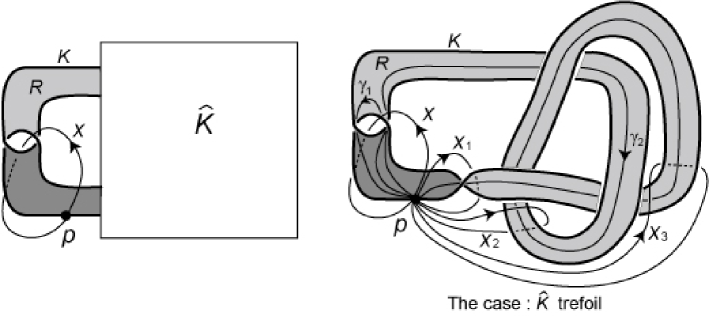
Figure 8. Doubled knot

¿From these data, we can give an admissible presentation of $\pi_{1}(M,p)$ as follows:

$$\pi_{1}(M,p)\cong\left\langle\begin{array}[]{c|c}\begin{array}[]{l}i_{-}(\gamma_{1}),i_{-}(\gamma_{2}),\\ x,x_{1},x_{2},\ldots,x_{l},\\ i_{+}(\gamma_{1}),i_{+}(\gamma_{2})\end{array}&\begin{array}[]{l}i_{-}(\gamma_{1})w_{1}x,i_{-}(\gamma_{2})w_{2},\\ r_{1},\ldots,r_{l-1},\\ i_{+}(\gamma_{1})x,i_{+}(\gamma_{2})xw_{3}\end{array}\end{array}\right\rangle,$$

where $w_{1},w_{2},w_{3}$ are words in $x_{1},\ldots,x_{l}$. The abelianization map $\rho:\pi_{1}(M)\to H_{1}(M)\cong\mathbb{Z}^{2}=\mathbb{Z}s\oplus\mathbb{Z}t$ is given by

$$x\mapsto s,\qquad x_{1},x_{2},\ldots,x_{l}\mapsto t.$$

A computation in matrices with entries in $\mathbb{Z}H_{1}(M)=\mathbb{Z}[s^{\pm},t^{\pm}]$ shows that

$$\sideset{{}^{\rho}\!\!}{}{\mathop{\begin{pmatrix}A\\ B\\ C\end{pmatrix}}\nolimits}=\bordermatrix{&i_{-}(\gamma_{1})w_{1}x&i_{-}(\gamma_{2})w_{2}&r_{1}&\ldots&r_{l-1}&i_{+}(\gamma_{1})x&i_{+}(\gamma_{2})xw_{3}\cr i_{-}(\gamma_{1})&1&0&0&\cdots&0&0&0\cr i_{-}(\gamma_{2})&0&1&0&\cdots&0&0&0\cr x&\ast&0&0&\cdots&0&s&\ast\cr x_{1}&\ast&\ast&a_{11}&\cdots&a_{1,l-1}&0&b_{1}\cr\vdots&\vdots&\vdots&\vdots&\ddots&\vdots&\vdots&\vdots&\cr x_{l}&\ast&\ast&a_{l1}&\cdots&a_{l,l-1}&0&b_{l}\cr i_{+}(\gamma_{1})&0&0&0&\cdots&0&1&0\cr i_{+}(\gamma_{2})&0&0&0&\cdots&0&0&1},$$

where $a_{ij}=\overline{\displaystyle\frac{\partial r_{j}}{\partial x_{i}}}$  coincides with the $(i,j)$-entry (applied an involution) of the Alexander matrix with respect to the Wirtinger presentation of $G_{\widehat{K}}$, and $b_{i}=\overline{\displaystyle\frac{\partial(i_{+}(\gamma_{2})xw_{3})}{\partial x_{i}}}$.

Recall that the matrix $\sideset{{}^{\rho}\!\!}{}{\mathop{\begin{pmatrix}A\\ B\end{pmatrix}}\nolimits}$ gives a representation matrix of $H_{1}(M,i_{+}(\Sigma_{1,1});\mathbb{Z}[s^{\pm},t^{\pm}])$. As a representation matrix, $\sideset{{}^{\rho}\!\!}{}{\mathop{\begin{pmatrix}A\\ B\end{pmatrix}}\nolimits}$ is equivalent to

$$\begin{pmatrix}a_{11}&\cdots&a_{1,l-1}&b_{1}\\ \vdots&\ddots&\vdots&\vdots\\ a_{l1}&\cdots&a_{l,l-1}&b_{l}\end{pmatrix}.$$

Therefore, if we apply the natural map $\mathbb{Z}[s^{\pm},t^{\pm}]\to\mathbb{Z}[t^{\pm}]$ $(s\mapsto 1)$ to each entry, we have an exact sequence

$$\mathbb{Z}[t^{\pm}]\longrightarrow H_{1}(G_{\widehat{K}},\{1\};\mathbb{Z}[t^{\pm}])\longrightarrow H_{1}(M,i_{+}(\Sigma_{1,1});\mathbb{Z}[t^{\pm}])\longrightarrow 0,$$

which shows that

(7.1) $$e(H_{1}(G_{\widehat{K}},\{1\};\mathbb{Z}[t^{\pm}]))\leq e(H_{1}(M,i_{+}(\Sigma_{1,1});\mathbb{Z}[t^{\pm}]))+1.$$

(Recall that the Alexander matrix of $\widehat{K}$ is a presentation matrix of $H_{1}(G_{\widehat{K}},\{1\};\mathbb{Z}[t^{\pm}])$.)

In the homology exact sequence

$$0\longrightarrow H_{1}(G_{\widehat{K}};\mathbb{Z}[t^{\pm}])\longrightarrow H_{1}(G_{\widehat{K}},\{1\};\mathbb{Z}[t^{\pm}])\longrightarrow H_{0}(\{1\};\mathbb{Z}[t^{\pm}])\longrightarrow H_{0}(G_{\widehat{K}};\mathbb{Z}[t^{\pm}]),$$

the fourth map is given by the augmentation map

$$H_{0}(\{1\};\mathbb{Z}[t^{\pm}])\cong\mathbb{Z}[t^{\pm}]\longrightarrow\mathbb{Z}\cong H_{0}(G_{\widehat{K}};\mathbb{Z}[t^{\pm}]),\qquad(t\mapsto 1),$$

whose kernel is $(t-1)\mathbb{Z}[t^{\pm}]\cong\mathbb{Z}[t^{\pm}]$, a free $\mathbb{Z}[t^{\pm}]$-module. Hence, we obtain an exact sequence

$$0\longrightarrow H_{1}(G_{\widehat{K}};\mathbb{Z}[t^{\pm}])\longrightarrow H_{1}(G_{\widehat{K}},\{1\};\mathbb{Z}[t^{\pm}])\longrightarrow\mathbb{Z}[t^{\pm}]\longrightarrow 0.$$

Then, by [24, Lemma 2.5], we have

(7.2) $$e(H_{1}(G_{\widehat{K}},\{1\};\mathbb{Z}[t^{\pm}]))=e(H_{1}(G_{\widehat{K}};\mathbb{Z}[t^{\pm}]))+1=m(\widehat{K})+1.$$

The conclusion follows from (7.1) and (7.2). ∎

Corollary 7.2.

There exist homologically fibered knots having Seifert surfaces of genus 1 with arbitrarily large handle number.

Proof.

It is known that there exist knots with arbitrarily large Nakanishi index. Our claim follows by combining this fact with Proposition 7.1. ∎

Example 7.3.

We present an example which shows the estimate of Proposition 7.1 is sharp.

Let $\widehat{K}$ be the pretzel knot $P(3,-3,3)=9_{46}$. The Nakanishi index of $\widehat{K}$ is 2 from the list in [25]. Let $K$ be a doubled knot along $\widehat{K}$ and let $\tau_{1}$ and $\tau_{2}$ (resp. $\tau^{\prime}_{1}$ and $\tau^{\prime}_{2}$) be the arcs whose ends are in $+$-side (resp. $-$-side) of the Seifert surface $R$ as illustrated in Figure 9.

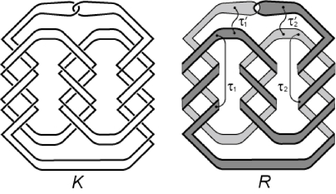
Figure 9. Doubled knot $K$ obtained from $P(3,-3,3)$

Let $(M,\gamma)$ be the complementary sutured manifold for $R$. Then we can observe that $({\rm cl}(M-N(\tau_{1}\cup\tau_{2}\cup\tau^{\prime}_{1}\cup\tau^{\prime}_{2})),\gamma)$, say $(\check{M},\gamma)$, is also a sutured manifold. Furthermore, we can show that $(\check{M},\gamma)$ is a product sutured manifold by using the technique of product decompositions (see Gabai [9]). This means that $(M,\gamma)$ has a Heegaard splitting $(W,W^{\prime})$ such that $h(W)=h(W^{\prime})=2$ where $\tau_{1}$ and $\tau_{2}$ (resp. $\tau^{\prime}_{1}$ and $\tau^{\prime}_{2}$) correspond to the attaching 1-handles of $W$ (resp. $W^{\prime}$). Thus we have $h(R)\leq 2$. (See [15] for the detail of this technique.) Therefore we have $h(R)=2$ by Proposition 7.1. Note that the Alexander polynomial of $K$ is equal to $t^{2}-t+1$, namely $K$ is homologically fibered.

References

[1]
G. Burde, H. Zieschang, Knots,
de Gruyter Studies in Mathematics, 5.
Walter de Gruyter Co., Berlin, 2003.
[2] T. Cochran, K. Orr, P. Teichner,
Knot concordance, Whitney towers and -signatures,
Ann. of Math. 157 (2003), 433–519.
[3]
R. Crowell,
Genus of alternating link types,
Ann. of Math. (2) 69 (1959), 258–275.
[4] R. Crowell, H. Trotter,
A class of pretzel knots,
Duke Math. J. 30 (1963), 373–377.
[5] D. B. A. Epstein,
Finite presentations of groups and -manifolds,
Quart. J. Math. Oxford 12 (1961), 205–212.
[6] S. Friedl,
Reidemeister torsion, the Thurston norm and
Harvey’s invariants,
Pacific J. Math. 230 (2007), 271–296.
[7]
S. Friedl, T. Kim,
The Thurston norm, fibered manifolds and
twisted Alexander polynomials,
Topology 45 (2006), 929–953.
[8]
D. Gabai,
Foliations and the topology of -manifolds,
J. Differential Geom. 18 (1983), 445–503.
[9]
D. Gabai,
Detecting fibred links in ,
Comment. Math. Helv. 61 (1986), 519–555.
[10]
D. Gabai,
Foliations and the topology of -manifolds. III,
J. Differential Geom. 26 (1987), 479–536.
[11]
S. Garoufalidis, J. Levine,
Tree-level invariants of three-manifolds, Massey products and
the Johnson homomorphism,
Graphs and patterns in mathematics and theorical physics,
Proc. Sympos. Pure Math. 73 (2005), 173–205.
[12]
H. Goda,
Heegaard splitting for sutured manifolds and Murasugi sum,
Osaka J. Math. 29 (1992), 21–40.
[13]
H. Goda,
On handle number of Seifert surfaces in ,
Osaka J. Math. 30 (1993), 63–80.
[14]
H. Goda,
Circle valued Morse theory for knots and links,
Floer homology, gauge theory, and low-dimensional topology, 71–99,
Clay Math. Proc., 5, Amer. Math. Soc., Providence, RI, 2006.
[15]
H. Goda,
Some estimates of the Morse-Novikov numbers for knots and links,
Carter, J. Scott (ed.) et al., Intelligence of low dimensional topology 2006,
World Scientific,
Series on Knots and Everything 40, 35–42, 2007.
[16]
H. Goda, M. Ishiwata,
A classification of Seifert surfaces for some pretzel links,
Kobe J. Math. 23 (2006), 11–28.
[17]
H. Goda, T. Sakasai,
Abelian quotients of monoids of homology cylinders,
Geometriae Dedicata 151 (2011), 387–396.
[18]
H. Goda, T. Sakasai,
Factorization formulas and computations of
higher-order Alexander invariants for homologically fibered knots,
J. Knot Theory Ramifications 20 (2011), 1355–1380.
[19] M. Goussarov,
Finite type invariants and n-equivalence of 3-manifolds,
C. R. Math. Acad. Sci. Paris 329 (1999), 517–522.
[20] N. Habegger,
Milnor, Johnson, and tree level perturbative invariants,
preprint.
[21]
K. Habiro,
Claspers and finite type invariants of links,
Geom. Topol. 4 (2000), 1–83.
[22] J. Harlander, J. A. Jensen,
On the homotopy type of CW-complexes
with aspherical fundamental group,
Topology Appl. 153 (2006), 3000–3006.
[23] N. V. Ivanov,
Mapping class groups,
Handbook of geometric topology, 523–633,
North-Holland, Amsterdam, 2002.
[24]
A. Kawauchi,
On the integral homology of infinite cyclic coverings of links,
Kobe J. Math. 4 (1987), 31–41.
[25]
A. Kawauchi (ed.),
A survey of knot theory, Birkhauser Verlag, Basel, 1996.
[26]
P. Kirk, C. Livingston, Z. Wang,
The Gassner representation for string links,
Commun. Contemp. Math. 3 (2001), 87–136.
[27] J. Y. Le Dimet,
Enlacements d’intervalles et torsion de Whitehead,
Bull. Soc. Math. France 129 (2001), 215–235.
[28]
J. Levine,